

Abstract
Although river discharge simulations from global hydrological models (GHMs) have undergone extensive validation, there has been less validation of reservoir operations, primarily because of limited observational data. Recent advancements in satellite remote sensing technology have facilitated the collection of valuable data regarding water surface area and elevation, thereby providing the ability to validate reservoir storage. In this study, we sought to propose a methodology for validation and intercomparison of monthly reservoir storage within GHMs simulations using two satellite-derived reservoir monitoring products, the Database for Hydrological Time Series of Inland Waters (DAHITI) and the Global Reservoir Surface Area Dataset (GRSAD). A pilot study was conducted for seven reservoirs in the contiguous United States (CONUS), with access to long-term ground truth data (the total catchment area accounts for around 9% of CONUS). We assessed two GHMs that participated in the inter sectoral model intercomparison project Phase 3a, H08 and WaterGAP2, with three distinct forcing datasets: GSWP3-W5E5 (GW), CR20v3-W5E5 (CW), and CR20v3-ERA5 (CE). The pilot study results indicate that for the seven reservoirs, WaterGAP2 generally outperforms H08. The CW forcing dataset demonstrated superior results compared with GW and CE, and DAHITI showed better consistency with ground observations than GRSAD if temporal coverage was sufficient. Overall, our study emphasizes the potential uses of satellite remote sensing data in reservoir storage validation and underscores the importance of normalization and decomposition techniques for improved validation efficacy.

Original content from this work may be used under the terms of the Creative Commons Attribution 4.0 license. Any further distribution of this work must maintain attribution to the author(s) and the title of the work, journal citation and DOI.
1. Introduction
Artificial reservoirs play an integral role in the hydrological cycle and water resource management (Grill et al 2019). Significant reservoirs have been incorporated into global hydrological models (GHMs) such as H08 (Hanasaki et al 2018), WaterGAP (Döll et al 2009), LPJmL (Biemans et al 2011), PCR-GLOBWB (Wada et al 2011), and CWatM (Burek et al 2020). GHMs enabled long-term physically-based consistent estimation of global hydrological variables from the past to the future. The complex, condition-dependent nature of reservoir operations (i.e. the storage and release of upstream water for downstream advantages) has led to the development and implementation of several algorithms into GHMs (Haddeland et al 2006, Hanasaki et al 2006). Consequently, validation and intercomparison of reservoir operations for these models are particularly important. Reservoir parameterization is indispensable in GHMs, particularly when they are applied for future projections.
When new reservoir operation algorithms were introduced (Haddeland et al 2006, Hanasaki et al 2006) and subsequently implemented into GHMs (Döll et al 2009, Biemans et al 2011, Wada et al 2011, Zhou et al 2016, Hanasaki et al 2018, Burek et al 2020), they were validated using in situ observations. Various model intercomparison projects have enabled an understanding of the relative benefits of specific models and algorithms (Telteu et al 2021). The inter-sectoral impact model intercomparison project (ISIMIP; Warszawski et al 2014) facilitates the intercomparison of numerous GHMs under uniform simulation settings. Several studies have validated and intercompared hydrological variables such as river discharge (Kumar et al 2022), irrigation water demand (Wada et al 2013), and terrestrial water storage (Pokhrel et al 2021). The first reservoir operation intercomparison was conducted by Masaki et al (2017), who examined the effects of dams on simulated river discharge. They found substantial variations in model simulations, but their research was restricted to the Green-Colorado River and the Missouri Mississippi River basins due to the global unavailability of observed gauged data. Reservoir operation modeling can only be improved by intensive validation and more information. Sadki et al (2023) validated and tuned their reservoir operation algorithm which is commonly employed in several GHMs . They applied their model to Spain, where abundant ground observations were available, demonstrating that historical reservoir operations could be well reproduced. Turner et al (2020) proposed a novel approach to predict reservoir operation in medium- to long-range forecasts, which utilized the intensively collected long-term historical reservoir records in the contiguous US. The remaining challenge is how we can extend such data collection globally in a practical manner to validate and subsequently improve the reservoir representation in GHMs.
Satellite remote sensing has emerged as a valuable tool for global validation, irrespective of geographical location (Alsdorf et al 2007). A few studies have developed methodologies to determine reservoir storage using satellite-derived altimetry and surface area data globally (Gao et al 2012, Busker et al 2019, Biswas et al 2021, Cooley et al 2021, Li et al 2021b, Biswas and Hossain 2022, Das et al 2022, Hou et al 2022, Li et al 2023). However, these datasets have not yet been used in multi-model intercomparison projects, primarily due to the lack of detailed information on the biases and errors at individual reservoirs and a universal reservoir ID to map reservoirs across datasets. Therefore, there remains a need to establish a method to systematically prepare satellite-based reservoir storage time-series data for global GHM validation.
Our research question is: how can we validate reservoir storage simulation results of GHMs with satellite-derived data? To answer this research question, we set two goals. First, we propose a method to prepare satellite-based reservoir storage time series data globally that can be directly compared to models. By the methodology developed by Gao et al (2012), Li et al (2023) and Busker et al (2019), we used remote sensing altimetry and surface area products to determine reservoir storage. Second, we conduct a pilot study to demonstrate the utility of this approach. We focused on seven strategically selected reservoirs across the Contiguous United States (CONUS), which enables us to conduct a complete cross-checking among data. We used the outputs of two GHMs that participated in ISIMIP Phase 3a (Frieler et al 2023) for stylized simulations of reservoir operations from 1901 to 2019. Because the objective of ISIMIP3a is to tell which GHMs or meteorological forcings perform better than others, we also derived preliminary answers from the pilot study. We also investigated the following specific questions on the method we proposed.
What are the challenges in preparing satellite-based reservoir storage data?
Do the findings on reservoir storage validation with satellite data align with ground observations?
Are some satellite products superior to others?
2. Materials and methods
2.1. Method
A method is presented below for systematically preparing satellite-based reservoir storage data directly comparable to GHM output. The data and methods used are a collection of earlier studies but are carefully selected for immediate use across the globe.
2.1.1. Data preparation 1: reservoir specification data
Reservoir parameters such as dam name, location (longitude and latitude), storage capacity (Sc ), and maximum surface area (Ac ) are provided in the ISIMIP3a protocol (Frieler et al 2023). These data are primarily obtained from the Global Reservoir and Dam Database (GRanD) v1.3, which was developed by the Global Water System Project (Lehner et al 2011). The data also include a set of dams provided by Dr Jida Wang from Kansas State University. This collaboration has resulted in a comprehensive database of 7330 dams, either constructed or under construction, spanning the years 286 to 2020. The cumulative global storage capacity of the database is approximately 7000 km3.
2.1.2. Data preparation 2: satellite data
As shown in the Introduction, monitoring reservoirs from space is a rapidly evolving study domain. Many studies have focused on one or a few reservoirs and applied the latest techniques for accurate, continuous, and frequent monitoring (e.g. Das et al 2022). Because our final goal was to validate GHMs globally at a decadal scale, we acquired data covering the globe for over 10 years. To the best of our knowledge, there are six datasets that meet this requirement, namely, Database for Hydrological Time Series of Inland Waters (DAHITI) (Schwatke et al 2015), Global Reservoir Surface Area Dataset (GRSAD) (Zhao and Gao 2018), Hydroweb (Crétaux et al 2011), G-REALM (Birkett and Beckley 2010), GloLakes (Hou et al 2022), and Biswas and Hossain (2022). We excluded Hydroweb and G-REALM because the number of reservoirs monitored is one or two orders of magnitude smaller than other datasets. GloLakes is promising but not used because it does not include many dams in CONUS (i.e. the name of only one in seven dams mentioned later was found in the database). We selected DAHITI and GRSAD because their data were easily accessible. It is important to note that in this article, DAHITI represents storage estimates based on satellite altimetry water level data of reservoirs/lakes, and GRSAD represents storage estimates based on optical remote sensing of surface water extents. It should be noted that new datasets are being produced by applying the latest satellite sensors. Among the other potential datasets, the Cooley et al (2021) dataset, which utilizes the ICESat-2 altimetry, is very promising, but we excluded it because it covers only 2018 and later.
2.1.2.1. DAHITI (surface water level time series)
The Database for Hydrological Time Series over Inland Waters (DAHITI) is a web service that offers valuable information on water levels, surface area, and volume variations in rivers, lakes, and reservoirs (Schwatke et al 2015, 2019 Busker et al 2019). DAHITI uses satellite altimetry technology to measure water levels in inland bodies, extending beyond its initial application in sea-level monitoring. The methodology utilizes an amalgamation of extended outlier rejection, a Kalman filter, and cross-calibrated multi-mission altimeter data. These data are collected from satellites such as Envisat, ERS-2, Jason-1, Jason-2, TOPEX/Poseidon, and SARAL/AltiKa, considering their respective uncertainties. This comprehensive approach facilitates a more accurate estimation of water level time series (Schwatke et al 2015). The data are available from 1992 to present. Temporal resolution varied within the period, but a simple monthly mean of the available data was considered in this study. In addition to water levels, DAHITI provides surface area time series for lakes and reservoirs, utilizing optical imagery (Schwatke et al 2019). In this study, however, we only used altimetry data from DAHITI to estimate reservoir storage, primarily because water surface area data were not universally available for all reservoirs under consideration.
2.1.2.2. GRSAD (surface area time series)
The GRSAD was created by Zhao and Gao (2018) and Gao and Zhao (2019). This dataset provides a monthly time series of water surface area data for 6,817 reservoirs worldwide, collectively representing a storage capacity of 6,099 km3 (Zhao and Gao 2018). The time frame of this dataset ranges from 1984 to 2015.
GRSAD builds upon the earlier work of Pekel et al (2016); it includes automatic corrections for disruptions caused by clouds, cloud shadows, and terrain shadows. The maximum surface area extent is determined based on a 500 m outward extension from GRanD shapefiles (Lehner et al 2011). As a result, any surface area beyond the 500 m threshold is not considered part of the reservoir. The dataset primarily uses 30 m Landsat satellite imagery; it does not incorporate data from other satellite sources. Although it provides extensive information regarding reservoir surface areas, it does not offer altimetry or volumetric change data.
2.1.2.3. Global Reservoir Bathymetry Dataset (GRBD) (bathymetry)
The GRBD constitutes another category of satellite product (Li et al 2020). This dataset employed a combination of satellite altimetry datasets, including ICESat, G-REALM, and Hydroweb, along with Landsat-based surface water datasets such as surface water occurrence (SWO) from global surface water (GSW, Pekel et al 2016) and monthly water area from GRSAD to create detailed bathymetry information for 347 reservoirs worldwide, representing approximately 50% of the global storage capacity. In addition to bathymetry data, GRBD offers valuable relationships such as area-elevation (i.e. the a and b parameters of equation (1) in section 2.1.3) and key reservoir parameters such as Sc .
2.1.3. Data processing: reservoir storage calculation from satellite data
For most reservoirs, as depicted in figure 1, there is a linear relationship between the water surface area (A) and the water surface elevation (h), represented as:

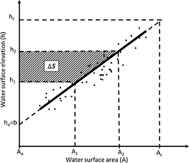
Figure 1. Relationship between the observed water surface area (A), water surface elevation (h), and the change in storage volume (, shaded region). The black dots depict the values of A and h for a hypothetical reservoir, while the thick solid black line represents the correlation within the observed range. This solid line can be extended in both directions to illustrate a hypothetical state ranging from an empty (h0, A0) to a full reservoir (hc and Ac ).

Download figure:
Standard image High-resolution imagewhere a and b represent the slope and intercept, respectively, obtained from a linear regression (Gao et al 2012, Busker et al 2019). These parameters are supplied by the GRBD dataset in our study (refer to table S1).
The volume change for a particular period is then calculated as the area of a trapezoid, as described by Gao et al (2012):

where ΔS represents the volume change, A1 and A2 are surface areas at the start and end of the period, and h1 and h2 are their respective water surface elevations.
Gao's method (Gao et al 2012) extended the linear relationship to reservoir storage capacity (Sc ) of the reservoir, resulting in the expression of the corresponding maximum surface area (Ac ) and maximum water surface elevation (hc ) as:

where Si represents the volume of water stored in the reservoir, corresponding to water surface area Ai and water surface elevation hi . However, hc records are, in most cases, missing in the reservoir specification inventories. Therefore, the storage estimation from GRSAD data is computed using the linear equation described in equation (1), as follows:

Busker's Method (Busker et al 2019) extends the linear relationship toward the minimum storage (i.e. zero storage); thus, the corresponding surface area is also zero, and the water surface elevation is the bed elevation of the reservoir,

Busker's method requires fewer parameters; Ac and hc are unnecessary. Additionally, the storage volume can be computed using only h or A by substituting the linear A–h relationship (equation (1):

Equation (6) is applicable for GRSAD and DAHITI datasets, which contain time series of surface area and elevation, respectively, within the context of our study. For values of 'a' and 'b', we utilized the GRBD database.
Li et al (2023) recently created the global reservoir storage (GRS) dataset which provides a monthly time series of water storage data for 7,245 reservoirs from 1999 to 2018. They convert the lake surface area time series of GRSAD into storage volume by the area-volume relationship derived from two bathymetry datasets. One is the GRBD for 347 reservoirs; the other is a new satellite-based estimation for the remaining 6,898. The essential difference from the storage derived from equation (6) and GRSAD is whether the relationship in bathymetry is linear or non-linear. In addition to the storage derived from GRSAD and DAHITI, we also used GRS in this study.
2.1.4. Data post-process
2.1.4.1. Normalization
The monthly storage time series can be normalized using the following equation:

where min(s) and max(s) represent the minimum and maximum values of the available monthly storage time series, respectively. By normalizing the monthly storage time series, information about the absolute value of reservoir storage is omitted; only the rate of change information is retained, enabling qualitative validation instead of quantitative.
2.1.4.2. Decomposition
The monthly storage time series (Sy,m ) can be decomposed (figure 2) into annual average storage (Sy ), mean annual seasonal variability (hereafter referred to as seasonal variability or ), and residuals (ey,m ), as follows:


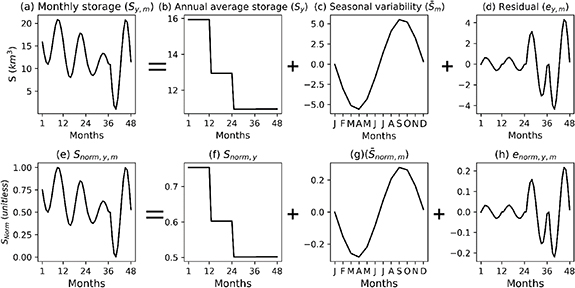
Figure 2. Components of volumetric storage investigated in this study. Raw (a)–(d) and normalized values (e)–(h).
Download figure:
Standard image High-resolution imageSy denotes a reservoir's annual average storage volume from January to December, computed by averaging the 12 monthly storage values. is determined by calculating the mean storage value for each month after subtracting the mean annual storage for that specific year; thus, it represents storage fluctuation within a year due to seasonal factors. ey,m constitutes the residual storage value after removing both the annual average storage and the seasonal variability, thus representing the storage component not attributable to annual or seasonal variations. Storage decomposition enables splitting the performance of GHMs for representation into annual storage and seasonal variability, which is helpful for reservoirs with carry-over storage capacity (i.e. storage capacity exceeds the mean annual inflow).

2.1.4.3. Evaluation metrics
Two metrics, Pearson's correlation coefficient (r) and Nash–Sutcliffe efficiency (NSE) (see supplementary text S1), were used to validate time series data. Any months corresponding to missing values in either observation or simulation were excluded from the validation process (the percentage of missing values will be reported later).
2.2. Pilot study
The previous subsection allows the preparation of satellite-based reservoir storage globally. This subsection describes a pilot study that uses these data. The pilot study aims to confirm the degree to which the prepared satellite-based reservoir storage values agree with ground observations and to perform a preliminary inter-model comparison. To achieve the first goal, the US, where the ground observations are readily available, was selected as the target site. To achieve the second goal, the results of the ISIMIP3a project, in which multiple GHMs are run under identical conditions, were used as modeled data.
2.2.1. Data preparation 1: modeled data
The third-round framework of the ISIMIP3a is focused on the evaluation and enhancement of impact models within the context of climate change (Frieler et al 2023). As of 9 June 2023, nine models have participated in the global water sector, but only two have completed simulations that include reservoir outputs. In this study, we utilized two GHMs, namely H08 and WaterGAP2 (WGP). H08 and WGP are the GHMs first incorporated reservoirs and participated in all phases of ISIMIP to date. It has been reported that H08 and WGP are almost at the center of the variation of various models in global water balance calculations (Haddeland et al 2011). We used three meteorological forcings that are bias-adjusted combinations of two reanalyzes, beginning in 1979 for ERA5 (European Centre for Medium-Range Weather Forecasts Reanalysis version 5) and W5 × 105 (WFDE5 over land merged with ERA5 over the ocean; the WFDE5 dataset was generated using the WATCH Forcing Data methodology applied to the surface meteorological variables from the ERA5), respectively (Lange et al 2022):
- 1.Global Soil Wetness Project Phase 3 (GSWP3) combined with W5E5 (GSWP3+W5E5, hereafter referred to as GW)
- 2.20th Century Reanalysis version 3 (20CRv3) combined with W5E5 (20CRv3+W5E5, hereafter referred to as CW)
- 3.20CRv3 combined with ERA5 (20CRv3+ERA5, hereafter referred to as CE)
These forcing data are globally available at 0.5° × 0.5° spatial resolution at daily intervals from 1901 to 2019. Combining the two models and three forcings yields six model simulations, with model and forcing names combined (e.g. H08 forced by GW results in H08_GW). Additional details regarding the simulation protocol can be found at https://protocol.isimip.org/ and in the work by Frieler et al (2023).
2.2.1.1. H08 model
The H08 model is a grid-cell-based GHM designed to address the impacts of human activities on the global hydrological cycle. H08 comprises six sub-models: land surface hydrology, river routing, reservoir operation, crop growth, environmental flow, and anthropogenic water withdrawal. The model was subsequently updated to include groundwater recharge and abstraction, aqueduct water transfer, local reservoir, seawater desalination, and return flow and delivery loss schemes (Hanasaki et al 2018). By incorporating these submodules and schemes, H08 simulates natural and anthropogenic hydrological processes at a spatial resolution of 0.5° on a daily scale by resolving water and energy balance. Specifically, H08 includes explicit flow regulation of 963 major global reservoirs. The modeling of release from the reservoir is based on the work of Hanasaki et al (2006). Reservoirs primarily used for irrigation are classified as irrigation reservoirs; all other reservoirs are considered non-irrigation reservoirs. The monthly release from irrigation reservoirs follows the downstream water demand. For non-irrigation reservoirs, the release is constant throughout the year. For both types of reservoirs, the interannual variation in storage is also reflected: release is greater when the storage at the beginning of a hydrological year is greater than the average, and vice versa. The water demand for irrigation reservoirs is presumably more affected by the seasonal cycle due to the seasonal nature of irrigation water requirements. Land surface parameters were optimized based on climatic zones using the method proposed by Yoshida et al (2022).
2.2.1.2. WaterGAP model
WaterGAP (WGP) is a GHM that comprises two primary components (Müller Schmied et al 2024). The WGP Global water use models calculate water use estimates for five sectors: irrigation, domestic, manufacturing, cooling water for electricity generation, and livestock. In contrast, the WGP global hydrology model uses water balance equations to calculate changes in water storage compartments and water flows between them. It considers fluxes such as groundwater recharge, evapotranspiration, river discharge, and net abstractions from surface water and groundwater, as calculated in a linking module from the sectoral water use models. Its calculations are performed with a daily time step. The reservoir operation has been described by Döll et al (2009) and Müller Schmied et al (2024). The reservoir algorithm follows the method of Hanasaki et al (2006), differentiating between reservoirs used for irrigation and other purposes and considering both reservoirs and regulated lakes. Contrary to the method of Hanasaki et al (2006), the annual release from a reservoir also depends on the long-term average mean streamflow of the grid cell where the reservoir is located, considering the water balance of the reservoir. In the model version used in ISIMIP3a (WaterGAP 2.2e), 1255 'global' reservoirs with storage volumes of ⩾0.5 km3 and 5722 'local' reservoirs (with smaller storage volumes) are included. However, only the global reservoirs are managed with the reservoir algorithm.
The primary aim of WGP is the provision of reliable estimates of renewable water resources on a global scale. To accommodate uncertainties in GHMs, a calibration routine is applied in WGP. This calibration ensures that the long-term annual simulated river discharge closely matches observed discharge within a ±10% tolerance at grid cells representing calibration stations. Calibration is performed using observed discharge data from a selection of 1509 discharge observation stations, which have been collated from three data sources (Müller Schmied and Schiebener 2022).
2.2.1.3. Reservoir operation in H08 and WGP
Reservoir operation has been integrated into both H08 and WGP. Nevertheless, these two models have notable similarities and distinctions, as outlined by Telteu et al (2021). Both models compute reservoir inflow, outflow, human water withdrawal, and storage. However, H08 accounts only for total runoff as the inflow component (Hanasaki et al 2018), whereas WGP factors in precipitation, groundwater, and return flow from human water use (Müller Schmied et al 2024). Furthermore, regarding outflow components, WGP incorporates evaporation and groundwater recharge from reservoirs, the considerations absent in H08.
2.2.2. Data preparation 2: ground observation data
Reservoir storage is always precisely monitored by dam operators, but the long-term time series are seldom published openly. This has been the primary obstacle in global reservoir modeling and analysis in the past. ResOpsUS (Steyaert et al 2022) is an exhaustive dataset containing historical information about reservoir inflows, outflows, and storage time series for 679 major reservoirs across the United States. The data, with daily temporal resolution, enable detailed analysis of reservoir dynamics. However, the temporal coverage varies among reservoirs based on factors such as construction date and data availability. The dataset spans 1930–2020, with the most robust data from 1980 to 2020. Notably, reservoirs in the dataset contain more than half of the total storage capacity of large reservoirs in the U.S., with a minimum storage threshold of 0.1 km3.
2.2.3. Reservoir selection
The process of identifying common reservoirs across H08, WGP, GRSAD, GRBD, and ResOpsUS datasets is streamlined by the shared use of the GRanD ID. This sharing facilitates the integration and comparison of data across the different datasets. However, DAHITI uses a unique identification system, thereby requiring individual examination of each reservoir for data availability. Accordingly, a meticulous selection procedure was conducted. First, common reservoirs among H08, WGP, GRSAD, GRBD, and ResOpsUS were identified, and there were 22 in total. This considerable shrink in the number of reservoirs is shown in the Venn diagram in figure 3. The shrink is primarily attributed to the availability of the bathymetry data of GRBD (i.e. data are available for 347 reservoirs globally) and the ground observation data of ResOpsUS (i.e. data are available for 679 reservoirs in the CONUS only). Then, they were searched on the DAHITI website. After a comprehensive review of data availability, only seven reservoirs listed in table 1 were found in all datasets and were thus selected as the foundation for analysis. The locations of these reservoirs in the H08 and WGP models within the 0.5° × 0.5° grids are indicated in table S2. Table S1 displays the storage capacity (Sc ) utilized in our study for these reservoirs. Identifying common reservoirs for all datasets is a prerequisite for this study, which evaluates the agreement between satellite products and the performance of GHMs. The starting and ending dates of ground observations for seven reservoirs in the ResOpsUs dataset are shown in table S3.
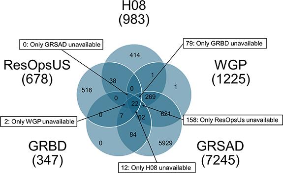
Figure 3. The Venn diagram of the number of dams seen in the five datasets, namely, H08, WGP, GRSAD, GRBD, and ResOpsUs.
Download figure:
Standard image High-resolution imageTable 1. Specifications of dams and corresponding reservoirs considered in this study. Year corresponds to the initial year of reservoir operation, Hdam corresponds to dam height, and Ac corresponds to the maximum water surface area of the reservoir (GRanD). Longitude and latitude indicate the location of the dams. GRBD adopts the identical ID to GRanD and HydroLAKES.
| Dam name | Lake name | GRanD ID | Hydro LAKES ID | DAHITI ID | River | Lon | Lat | Year | Hdam (m) | Ac (km2) | Main purpose |
|---|---|---|---|---|---|---|---|---|---|---|---|
| Hoover | Lake Mead | 610 | 809 | 204 | Colorado River | −114.74 | 36.02 | 1935 | 223 | 580.95 | Water supply |
| Glen Canyon | Lake Powell | 597 | 802 | 107 | Colorado River | −111.49 | 36.94 | 1963 | 216 | 120.75 | Hydro-electricity |
| Fort Peck | Fort Peck Lake | 307 | 721 | 11 112 | Missouri River | −106.41 | 48.00 | 1957 | 78 | 814.09 | Flood control |
| Toledo Bend | Toledo Bend Lake | 1269 | 838 | 10 247 | Sabine River | −93.57 | 31.17 | 1966 | 34 | 599.62 | Hydro-electricity |
| Structure 193 | Lake Okeechobee | 1957 | 69 | 57 | Taylor Creek | −81.10 | 26.94 | 1972 | 11 | 1418.77 | Flood control |
| Wesley E. Seale | Lake Corpus Christi | 1317 | 9615 | 13 139 | Nueces River | −97.87 | 28.05 | 1958 | 25 | 59.14 | Recreation |
| Coolidge | San Carlos Lake | 656 | 9440 | 13 130 | Gila River | −110.52 | 33.18 | 1929 | 77 | 15.47 | Irrigation |
2.2.4. Analysis
Initially, satellite data were compared with ground observations to determine compatibility with evaluations of model simulations. Subsequently, simulated reservoir storage from the two ISIMIP3a models, H08 and WaterGAP, was validated against two satellite datasets, GRSAD and DAHITI. Reservoir storage data were examined in raw, normalized, and decomposed. Refer to table 2 for the data utilized.
Table 2. Reservoir storage data used in this study. Different datasets and methods utilized to calculate S with GRSAD lead to the same normalized storage because the resulting volumes are linearly proportional.
| Category | Name (description) | Acronym | |
|---|---|---|---|
| GHMs | H08 | H08 | |
| WaterGAP2.2e | WGP | ||
| Input forcings | GSWP3 + W5E5 | GW | |
| 20CRv3 + W5E5 | CW | ||
| 20CRv3 + ERA5 | CE | ||
| Simulations | e.g. H08 forced by GW | H08_GW | |
| Ground observation | ResOpsUS | Grd_obs | |
| Raw storage | Normalized storage | ||
| Reservoir volume from satellite data | GRSAD area + Sc from GRBD + Gao's Method | GRSAD_GRBD | GRSAD |
| GRSAD area + Sc from ISIMIP + Gao's Method | GRSAD_ISIMIP | GRSAD | |
| GRSAD area + Busker's Method [Sc not needed] | GRSAD_Busker | GRSAD | |
| DAHITI elevation + Busker's method [Sc not needed] | DAHITI_Busker | DAHITI | |
| GRS (Li et al 2023) | GRS | GRS | |
We analyzed the data at a monthly interval for two reasons. First, we understand that the latest satellite product can estimate the sub-monthly dynamics of reservoir storage. Even though GHM simulations can be run on a daily scale, the ISIMIP3a simulation protocol foresees only monthly resolution of nearly all variables to avoid excessive data storage and data transfer demand. Second, as Masaki et al (2017) clearly show, GHMs have still observed substantial differences in monthly simulations among models. These differences stand out clearly when the catchment area is relatively small or multiple reservoirs are cascading. For a global simulation at a spatial resolution of half a degree, we considered a monthly resolution largely valid.
3. Results and discussion
In this section, we report the findings from the pilot study. section 3.1 discusses the satellite data utilized in this study. We focus on some of the post-processes, notably the area-elevation-volume conversion, which brings considerable uncertainty. This subsection is associated with the first specific research question: What are the challenges in preparing satellite-based reservoir storage data? section 3.2 presents the validation of simulated reservoir storage from ISIMIP3a against two satellite-derived reservoir storages and ground observation data. This subsection is associated with the second and the third specific research questions: do the findings on reservoir storage validation with satellite data align with ground observation? Are some satellite products superior to others? Lastly, section 3.3 offers an overview of the uncertainties associated with estimating reservoir storage and related data.
3.1. Satellite data utilized in this study
3.1.1. Monthly reservoir storage
The monthly time series of storage volume for the seven selected reservoirs (reservoir storage, S) from two remote sensing datasets were compared with ground-based observations (figure 4). The volumes calculated using satellite data (GRSAD and DAHITI) significantly fluctuated depending on the data source and the calculation method (i.e. Busker's method or Gao's method) utilized for raw storage (figures 4(a)–(g)). Intriguingly, even when the same surface area data from GRSAD were used, the storage estimates varied according to the methodologies adopted (i.e. GRSAD_GRBD, GRSAD_ISIMIP, and GRSAD_Busker, represented by gray lines). However, after normalization, the satellite-derived reservoir volumes aligned well with ground observations (figures 4(h)–(n)).
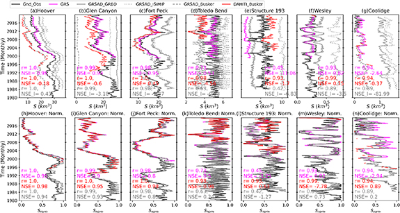
Figure 4. Monthly reservoir storage from satellite data and ground observation. Raw monthly reservoir storage (a)–(g) and normalized storage (h)–(n) for the seven selected US reservoirs from ground observation (black) and two satellite data GRSAD (gray), GRS (pink), and DAHITI (red). For GRSAD, three volumes are obtained by different combinations of data and methods (table 2). Correlation coefficients (r) and NSE values for GRSAD_GRBD, GRS, and DAHITI_Busker are shown in the figure and tables S4 (raw) and S5 (normalized). Note that three GRSAD lines are indistinguishable in panels h–n due to normalization.
Download figure:
Standard image High-resolution imageSeveral factors contribute to the variances in satellite-derived S, utilizing different methods and data. For instance, the difference between S derived from GRSAD_ISIMIP and GRSAD_GRBD (see table S1) can be attributed to the varying reservoir storage capacities used. Intriguingly, S calculated using Busker's method (GRSAD_Busker), which does not consider the maximum storage parameters such as Ac, hc , and Sc , was closest to the observed storage.
The raw storage volume (S) calculated using DAHITI_Busker and GRSAD_Busker displayed considerable agreement for Hoover, Fort Peck, Toledo Bend, and Coolidge (figures 4(a), (c), (d) and (g)). This agreement is promising because these calculations used entirely different satellite products: surface area imagery and water level altimetry. However, discrepancies were evident for Glen Canyon and Structure 193 (figures 4(b) and (e)). For Glen Canyon, temporal storage variability was lost when surface area data from GRSAD were used but not when surface elevation data from DAHITI were used. With the significant differences in surface area parameters between GRSAD and GRBD, the estimation of the linear A–h relationship for Glen Canyon has limitations (Li et al 2021a). The issue stems from the lake polygon included in the GRanD database. Manual correction was applied to GRBD (i.e. slope a and interception b) but not to GRSAD (i.e. monthly lake area A), resulting in inconsistencies.
Structure 193, also known as Lake Okeechobee, had a shallow average depth of 2.7 m but an extensive surface area (1418.77 km2). Therefore, its A–h relationship differed considerably from the schematic shown in figure 1, such that the A–h relationship had a very small value for 'a' and 'b' was negative (equation (1), table S1).
As seen in the panels for the Wesley and Coolidge Dams, the temporal coverage of DAHITI is rather limited (figures 4(f), (g), (m) and (n)). Because the overlap between DAHITI and ground observation is too short, the normalization does not account for the temporal variations over the long ground observation period. Therefore, the NSE score deteriorates on normalization. For such cases, statistics should be viewed with care.
In summary, the raw satellite-based storage time series exhibited considerable uncertainty due to reservoir surface area, the parameters a and b (figure 1), hc and Ac , and temporal coverage. The success in normalization is mainly due to the proportionate contraction and expansion of the water surface area to different elevations if a significant portion of the total water surface area is monitored. Consequently, a simple normalization enables effective qualitative validation, including signs of change and timing of high/low peaks, of the abilities of hydrological models to simulate reservoir operations.
GRS, one of the latest global satellite storage products, shows remarkably less biased storage estimation, particularly for the Hoover, Glen Canyon, Fort Peck, and Toledo Bend dams (figures 4(a)–(d)). However, there are some systematic discrepancies in the Structure 193, Wesley, and Coolidge dams (figures 4(e)–(g)). After normalization, GRS overlaps with GRSAD (figures 4(h)–(n)). This is not surprising because they commonly used the GRSAD lake area database. Because GRSAD covers a longer temporal duration, hereafter, we analyze only GRSAD.
3.1.2. Decomposed monthly reservoir storage from satellite and ground observation
The normalized time series for satellite-derived and ground-based volumes were decomposed into annual mean storage, seasonal variability, and residuals (figure S1). The correlation coefficient and NSE are displayed in table S6. For reference, the decomposed raw storage (S) is depicted in figure S2.
Overall, satellite-derived decomposed storage components (annual storage, seasonal variability, and residual) consistently compared well with ground-based observation storage components (details in supplementary text S2); correlation (>0.7) and NSE (>0.5) values were high (Moriasi et al 2007). In most cases, annual storage performed prominently among the decomposed components, particularly for GRSAD-based Snorm (table S6).
These satellite-derived components of decomposed normalized monthly storage compared well against their ground observation counterparts and are suitable for validation of model simulations. DAHITI is highly reliable when sufficient, continuous data are available (for instance, data for >5 years). When DAHITI data is unavailable or limited, GRSAD remains a viable (although less robust) alternative. Short-term data (<3 years) and highly discontinuous data, such as Wesley for DAHITI and Coolidge for ground observation, should not be used for validation.
3.2. Validation of simulated reservoir storage from ISIMIP3a
For the sake of a complete cross-validation among products, we conducted a pilot study by limiting the sample size, as discussed in section 2.2. The following subsubsections compare the annual storage and seasonal variability, using the normalized time series of monthly reservoir storage from two ISIMIP3a participating models, with their respective counterparts from two satellite products. Then, the consistency of the validation metric evaluated against satellite data is compared with the consistency of ground observations.
3.2.1. Monthly storage
The model simulations were reasonably consistent with satellite-based observations for Snorm,y,m (figures 5(a)–(g)). In particular, simulations for Fort Peck had high correlations with GRSAD and DAHITI. On average, the model performed better when compared with GRSAD than with DAHITI (figures 5(h) and (i)). Particularly, Snorm,y,m for Structure 193 performed well against GRSAD and poorly against DAHITI. Exceptionally, for Toledo Bend (figure 5(d)), performance relative to DAHITI surpassed GRSAD (figures 5(h) and (i)).

Figure 5. Validation of simulated monthly normalized reservoir storage. (a)–(g) Model simulations compared with satellite data and ground truth for monthly normalized reservoir storage. Color shading indicates mean variation among three forcing datasets, representing sensitivity to input forcings (), for H08 (yellow) and WGP (blue). (h)–(j) Average correlation coefficient with three evaluation storage datasets: GRSAD, DAHITI, and ground observation, respectively, for each reservoir (a)–(g). Colors indicate correlation classification. Values in square brackets indicate the percentage temporal coverage of reservoir storage from 01/1980 to 12/2019 for each reservoir's evaluation data. Reservoirs with hatch marks had <30% coverage and were not included in subsequent analyzes.

Download figure:
Standard image High-resolution imageTo illustrate how our proposed method will be finally used, we present a preliminary model and forcing data intercomparison. The performance of WGP ( > 0.5 for 8/12) was superior to the performance of H08 ( > 0.5 for 4/12) (figures 5(h) and (i)). Compared with WGP, H08 was generally more sensitive () to input forcings (figures 5(a)–(g), S3 and table S7). Among the three forcings, GW ( > 0.5 for 7/12) and CE ( > 0.5 for 7/12) performed better than CW ( > 0.5 for 6/12). A direct comparison of r between CE and GW showed that CE had higher values (CE > GW for 7/12). Noteworthy is the decline in simulation performance since 2005 for unclear reasons. Because most of the DAHITI data included this period, performance relative to GRSAD is generally poor. Considering its long-term consistent coverage, GRSAD demonstrates better consistency with ground observations (i.e. figure 5(h) displays better alignment with figures 5(j) than (i)). Thus, in validating Snorm,y,m for ISIMIP3a, GRSAD is a more reliable evaluation data source than DAHITI when considering the seven reservoirs in this study.


3.2.2. Annual average storage
The annual storage simulations were consistent with satellite observations in most cases (figure 6). In particular, Fort Peck and Coolidge simulations demonstrated good agreement with both DAHITI and GRSAD (figures 6(c) and (g)). For most reservoirs, the average correlation coefficient was >0.5 for simulations across two models and three forcings compared with GRSAD (figure 6(h)); this finding was consistent with results from ground observation comparisons (figure 6(j)). We only used GRSAD for further comparisons of GHMs and forcings in this subsection because there were apparent discrepancies between DAHITI and ground observations (figures 6(i)–(j)). This is because more than 50% of DAHITI data covers the period after 2005, when the model's performance deteriorated (section 3.2.1). Because of the difference in the validation period, the results of GRSAD and DAHITI were incomparable.
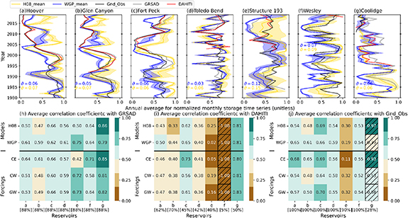
Figure 6. Validation of simulated annual average normalized reservoir storage. Same as figure 4 but for annual average normalized reservoir storage (Snorm,y ).
Download figure:
Standard image High-resolution imageFrom figure 6, the model and forcing data intercomparison goes as follows. The performances of the two GHMs concerning Snorm,y correlations with satellite data were nearly equivalent; WGP ( > 0.5 for 7/7) was slightly superior to H08 ( > 0.5 for 6/7) (figure 6(h)). Additionally, H08 displayed a slightly larger standard deviation than WGP (figures 6(a)–(g)), indicating that it had substantially more interannual variability with input forcings. Among the input forcings, CE performed best in terms of the correlation coefficient, followed by GW and CW. WGP_CE correlation coefficients were considerably higher than the correlation coefficients of other GHM-Forcing combinations for most satellites (figure S4).


The GHMs readily captured the interannual variation of reservoir storage.
3.2.3. Seasonal variability
The model simulations adequately captured the seasonal cycle of reservoir storage in many instances (figure 7). The correlations of simulations with both satellite datasets were generally high, such that many values exceeded 0.5 (21/35 for GRSAD and 24/35 for DAHITI), except for the Hoover and Wesley dams. For instance, the simulated peak timing of the Hoover Dam (April) lagged the satellite products (from January to March) by 1–3 months, resulting in weaker correlations.
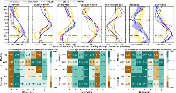
Figure 7. Validation of simulated monthly seasonal variability of normalized reservoir storage. Same as figure 4, but for seasonal variability of normalized reservoir storage (Snorm,m ). For Wesley (f), the DAHITI-derived storage is fully represented in figure S1m.
Download figure:
Standard image High-resolution imageBoth H08 ( > 0.5 for 9/14) and WGP ( > 0.5 for 8/14) performed particularly well in terms of simulating monthly variability in most reservoirs (figures 7(h) and (i)); WGP was superior to H08 (for 9/14 cases). H08 demonstrated less robust performance for the Hoover and Wesley Dams, but WGP displayed relatively strong correlations with observations for these reservoirs. Therefore, WGP demonstrated superior overall performance compared with H08. Moreover, H08 exhibited more significant variability according to input forcings than WGP. Among the input forcings (figures 6(h) and (i)), GW simulations ( > 0.5 for 11/14) outperformed CW ( > 0.5 for 9/14) and CE ( > 0.5 for 8/14). Even in terms of r values, GW performed best for 8/14 cases among the three forcings (figures 6(h) and (i)). This result is consistent with the evaluation relative to ground observations, where 5/7 reservoirs had the highest correlation for GW (figure 7(j)).


A comparison of simulations showed that DAHITI and GRSAD aligned with ground observations; DAHITI demonstrated relatively better consistency. We observed two instances of contradictory outcomes. First, WGP validation for the Fort Peck Dam and the Toledo Bend Dam, where a weak correlation with GRSAD differed from a strong correlation with DAHITI. Cases with very short data availability periods, such as Wesley and Coolidge for DAHITI, should be excluded from validation. In these instances, GRSAD should be used because it can appropriately capture the seasonal variation due to its long-term data availability. However, when DAHITI has sufficient temporal coverage, it outperforms GRSAD. Second, the H08-WGP comparison for Structure 193. In this case, the simulated seasonal cycle of WGP for Structure 193 closely correlated with GRSAD, but the amplitude was considerably smaller. These discrepancies lead to questions regarding the reliability of a single evaluation data source. Therefore, in the absence of ground-based observations, multiple satellite data products and metrics should be used to increase confidence in validation and intercomparison results. When a sufficient number of reliable satellite products were available, it would be possible to calculate the mean and ranges of satellite data ensemble.
3.3. Discussion
We discuss uncertainties and implications based on the pilot study. Although the findings cannot be generalized because of the limited sample size (two models and seven reservoirs), we still believe the contents are helpful for fully implementing our model for the forthcoming extensive global model validation studies.
3.3.1. Uncertainties
This study inherited some uncertainties from the previous efforts on satellite monitoring of reservoirs. There were four main issues. First, we assumed a linear A–h relationship for reservoir storage. This relationship is not genuinely linear, particularly when the reservoir is near full or empty. Many existing approaches require knowledge of water surface elevation at storage capacity; such information is not currently available in published global reservoir inventories. Monitoring Sc and hc from space is challenging because the water level of operational reservoirs has very little opportunity to reach the exact total capacity. The bathymetry approach (e.g. Messager et al 2016) also does not provide information about the water level at total capacity unless other methods specify the highest shoreline. Therefore, significant uncertainties may arise when calculating reservoir storage using these parameters (Gao et al 2012). It should also be noted that A–h relationship is not necessarily constant and subject to change due to exceptional events. Furthermore, the records in the inventories are not necessarily error-free or consistent with information in other inventories. This indicates a need for extensive quality checks among global reservoir inventories. Due to these issues, we abandoned using absolute storage estimates and normalized them. Although we showed that the timing and rate of rise and fall can be validated, a significant limitation of our study was the loss of storage magnitude information. The GRS database (Li et al 2023) adopts a more realistic and non-linear A–h relationship in converting lake area data into storage. As seen in figure 4, GRS outperforms the products with a linear assumption. Improvements in bathymetry estimation are the key to addressing this problem. Second, the limitations of area-based satellite products (i.e. GRSAD). Discrepancies in the consideration of water surface area extents (i.e. distinguishing between reservoir and river), as noted in the case of the Glen Canyon Dam (section 3.1.2), lead to concerns about the reliability of water surface area datasets. Third, there are limitations to altitude-based satellite products (i.e. DAHITI). This study found that DAHITI agrees better with the ground observation than GRSAD, but the advantage is largely deteriorated by its high frequency of missing data. Further technical advancement in data processing is expected for more extensive spatio-temporal coverage of this type of data. Finally, since 2005, there has been a clear discrepancy between simulation results and ground observations. This issue should be further examined from various aspects, including validation with other variables and at different locations.
3.3.2. Implications
Model intercomparison aims to identify the superior model among members and the reasons for superiority. The implications earned from our pilot study are summarized as follows.
First, in general, it is challenging to identify the superior model. We learned that the model and forcing performance vary according to the reservoirs. Increasing the number of reservoirs is a prerequisite of model intercomparison to avoid drawing erroneous conclusions by chance. The performance also varies by the spatio-temporal scale. Generally, the discrepancies among forcing data are relatively minor at a continental and monthly scale but exhibit significant variations at a catchment and daily scale. A detailed analysis will be performed in the forthcoming papers with more models and greater spatial coverage.
Second, it is difficult to single out the performance of the reservoir operation scheme because the simulation performance is dependent on the overall hydrological simulation (i.e. the daily water balance calculation carried out by the land surface hydrology and the river routing sub-models in GHMs.) For instance, the superior performance of WGP over H08 could be attributed to the calibration of river discharge (see section 2.2.1), which enhances the overall accuracy of reservoir inflow and outflow estimates in WGP. It could also be attributed to the fact that H08 tends to produce more significant temporal variation in storage than WGP (i.e. the sigma in figures 5, 6 and table S7). The performance metric tends to drop largely for models with the former tendency when the phase was incorrectly simulated. Furthermore, GHM performance cannot be determined by storage volume alone because it is affected by inflows and outflows.
Three additional approaches are considered for comprehensive intercomparison and validation of GHMs. The first approach is a systematic offline intercomparison. The performance of individual reservoir operations algorithms can be compared by applying them on a stand-alone basis at specific reservoirs for which reliable inflow, outflow, and storage data are available. The obvious drawback is that this approach is only applicable to data-rich regions. The second approach is a systematic online intercomparison. By implementing multiple reservoir operation algorithms in each GHM, modelers can identify the impact of the reservoir operation algorithms on their simulations. The disadvantage is that this approach requires intensive coding and more simulation runs. The final approach is a cross-validation. By adding more validation variables, e.g. river discharge upstream and downstream of a reservoir, it is possible to infer whether the simulated inflows and releases are overestimated.
4. Conclusions
In this study, to validate the long-term reservoir storage output of GHMs, we proposed a method for estimating monthly reservoir storage from satellite information that can be applied globally. A pilot study was conducted to examine the effectiveness of the method.
Our first research question was, 'What are the challenges in preparing satellite-based reservoir storage data?' The applicability of our method is primarily constrained by the limited availability of reservoir bathymetry data GRBD. Although water surface-area or water level altimetry time series are extensively available, an A–h relationship is needed to convert them into storage volume. In addition, we found that the satellite products can be used as a surrogate for ground truth when two key criteria are met. (1) The satellite and simulation data should be normalized before comparison because there is significant uncertainty when converting raw satellite observations (i.e. water surface area and water level altimetry) into absolute reservoir storage volumes. Although magnitude information is lost, the data provide invaluable information on the timing and rate of rise and fall globally. (2) The satellite observation period must be sufficiently long (i.e. 5 years) to correctly capture long-term trends and sample monthly storage variation. The second question was, 'Do the findings on reservoir storage validation with satellite data align with ground observation?' Although the number of samples studied was limited, we found general agreement between satellite-based and ground observation-based validation results in the pilot study, indicating overall reliability. The third question was, 'Are some satellite products superior to others?' Comparisons of DAHITI (altimetry-based data) and GRSAD (water surface area-based data) revealed that altimetry-based data demonstrates better consistency with ground observations if temporal coverage is sufficient. This is a recurring observation because all reservoirs undergo storage changes reflected in elevation alterations detectable by altimeters (Busker et al 2019, Verma et al 2021). However, the same is not valid for surface area changes unless the reservoir is particularly large and has no complex dendritic shape. The effectiveness of specific satellite data in tracking changes in surface area or volume is greatly influenced by factors such as the reservoir shape, shoreline characteristics, climate, and the surrounding terrain. However, with respect to simulations, the extended temporal coverage of GRSAD provides better agreement with ground observations for annual storage and residuals. Therefore, multiple satellite datasets should be utilized for model validation and intercomparison efforts to increase confidence in the results.
The pilot study also showed the preliminary results of model validation. For seven reservoirs in CONUS, two ISIMIP3a models, H08 and WGP, demonstrated satisfactory performance in normalized annual average storage and seasonal variabilities. Within the limited cases the pilot study covered, we found that WGP demonstrated slightly better performance overall than H08 (figures 4–6), although differences between the two models were minor. Considering the forcing data, CE and GW exhibited the best annual storage and seasonal variability performances, respectively.
To our knowledge, this study is the first effort to propose using multiple satellite-based products to validate and intercompare multiple model simulations (GHM and forcing combinations) for reservoir operations across forcings on a continental scale. Reservoir operation records are often not disclosed, especially for basins that flow across more than one country (Vu et al 2022). Our study demonstrated the feasibility of extending the spatial coverage of validation and intercomparison globally.
To facilitate further research and applications, we offer four recommendations. First, the latest satellite techniques must be incorporated to reduce the uncertainties discussed in section 3.3. Advanced data are being produced by developers (Cooley et al 2021, Hou et al 2022, Li et al 2023), and with the launch of the SWOT mission, the potential for satellite-based surface water tracking is poised to expand significantly (Biancamaria et al 2016). This ongoing effort to enhance satellite-based validation will yield more reliable reservoir storage assessments and predictions (Sadki et al 2023, Zhao et al 2024, Baratgin et al 2024, Salwey et al 2024). Second, more models and forcings should be included to enhance the comprehensiveness of the study by expanding the ensemble of simulations. Third, although this study exclusively focused on the CONUS region (i.e. for the sake of rigorous validation, we only studied reservoirs for which historical reservoir operation records were available in the ResOpsUS database that covers the contiguous US only), future studies should be performed globally, including reservoirs without ground observations. Different tendencies in data and models may be obtained from this study when the study area is expanded. Finally, an integrated platform combining multiple satellite products with a standard ID is needed to synchronize reservoirs and lakes with existing inventories such as GRanD and Hydrolakes.
Acknowledgment
This research was supported by the Japan Society for the Promotion of Science (KAKENHI; Grant Numbers 21H05002 and 22H01604).
Data and code availability statement
The data that support the findings of this study are openly available at the following URL/DOI: https://doi.org/10.5281/zenodo.8291850.
Conflict of interest
The corresponding author declares that neither they nor their co-authors have any competing interests.