

Abstract
The complex stratification of tropical forests is a key feature that directly contributes to high aboveground biomass (AGB) and species diversity. This study aimed to explore the vertical patterns of AGB and tree species diversity in the tropical forest of Pasoh Forest Reserve, Malaysia. To achieve this goal, we used a combination of field surveys and drone technology to gather data on species diversity, tree height (H), and tree diameter at breast height (D). As all trees in the 6 ha plot were tagged and identified, we used the data to classify the taxonomy and calculate species diversity indices. We used unmanned aerial vehicle-based structure-from-motion photogrammetry to develop a Digital Canopy Height Model to accurately estimate H. The collected data and previous datasets were then used to develop Bayesian height–diameter (HD) models that incorporate taxonomic effects into conventional allometric and statistical models. The best models were selected based on their performance in cross-validation and then used to estimate AGB per tree and the total AGB in the plot. Results showed that taxonomic effects at the family and genus level improved the HD models and consequent AGB estimates. The AGB was the highest in the higher layers of the forest, and AGB was largely contributed by larger trees, especially specific families such as Dipterocarpaceae, Euphorbiaceae, and Fabaceae. In contrast, species diversity was the highest in the lower layers, whereas functional diversity was the highest in the middle layers. These contrasting patterns of AGB and species diversity indicate different roles of forest stratification and layer-specific mechanisms in maintaining species diversity. This study highlights the importance of considering taxonomic effects when estimating AGB and species diversity in tropical forests. These findings underscore the need for a more comprehensive understanding of the complex stratification of tropical forests and its impact on the forest ecosystem.
Export citation and abstract BibTeX RIS

Original content from this work may be used under the terms of the Creative Commons Attribution 4.0 license. Any further distribution of this work must maintain attribution to the author(s) and the title of the work, journal citation and DOI.
1. Introduction
One of the most prominent features of tropical forests is their complex stratification. The top canopy consists of tall trees, which sometimes reach over 60 m in height, and the layers under the canopy are complex (Ashton and Hall 1992, Richards 1996). This complex vertical forest structure produces heterogeneous environmental conditions under the canopy; thus, this complexity expands the habitat for different species, reduces the interspecific competition, and enables coexistence of many species (Laurans et al 2014). High species diversity in tropical forests results, at least in part, from its complex and high degree of forest stratification. Furthermore, a higher forest canopy directly contributes to storing a higher amount of aboveground biomass (AGB) (Ali and Yan 2017, Bordin et al 2021). Thus, forest canopy height and stratification are closely linked ecologically with both species diversity and AGB (Xu et al 2020), which indicates that the vertical forest structure is an essential component of AGB and species diversity. The vertical patterns of AGB and species diversity are not yet well understood, but it is expected that higher canopy trees significantly contribute to the total AGB in a forest, whereas the species diversity is largely the result of small trees on the forest floor. These contrasting vertical patterns between AGB and species diversity suggest different roles in forest layers (Cavalieri et al 2010, Jin et al 2014). Furthermore, identifying the taxonomy for the stratification, AGB, and species diversity is crucial to understanding the background mechanisms of maintenance of ecosystem functions and species diversity, as well as for effective forest management and conservation.
The estimation of AGB in tropical forests has long been a core issue in tropical forest ecology in terms of resource assessment and, more recently, climate change (Kato et al 1978, Yamakura et al 1986, Ketterings et al 2001). Conventional models for estimating AGB use two essential variables: tree height (H) and tree diameter (D). Among these two variables, D is typically available in the field data, such as from permanent forest plots, whereas H is relatively difficult to measure accurately. Thus, previous studies have first tried to develop the tree height–diameter (HD) allometric and statistical models to estimate H from the observed D, and then the models were used for all stand-level data to obtain estimated H (Ogawa et al 1965, Malhi et al 2006, Pan et al 2011, Chave et al 2014).
However, two difficulties persist in developing HD models. First is the lack of accurate H measurements, especially in tall trees; specifically, it is difficult in the field to measure the accurate H of tall trees from the forest floor, e.g., using clinometers, laser rangefinders, or hypsometers (Sullivan et al 2018). Likely the most direct and accurate approach to H measurement would be a destructive sampling of the trees, a method used in previous studies in the 1970s (Kato et al 1978). Because this approach is a highly destructive, high-cost, and unrepeatable method, it is not sustainable or feasible in current studies. The second difficulty is the lack of taxonomic consideration in conventional HD models, although it has been pointed out that most HD relationships are species-specific (Cole and Ewel 2006). One reason for this difficulty is the limited species sample size because the tree density of each species is usually quite low in tropical forests, especially for larger trees.
Recent advances in unmanned aerial vehicles (UAVs), remote sensing (RS), and their mounted sensors, along with analytical technologies, have enabled researchers to overcome these challenges without resorting to destructive sampling. In fact, the successful assessment of indices relevant for species diversity, H, and AGB using UAVs and/or RS has already been achieved. For example, light detection and ranging (LiDAR) technology has been used to measure H and estimate AGB (Duncanson et al 2017, Beland et al 2019). Multispectral sensors on UAVs and RS integrating in situ field species diversity data have been used to measure components of biodiversity by calculating a proxy index of multispectral waves related to species diversity (Fassnacht et al 2022, Kacic and Kuenzer 2022), although these complex sensors are expensive. Structure-from-motion photogrammetry technology combined with UAVs, termed the UAV-based structure-from-motion (UAV-SfM) approach, utilizes images captured by UAVs equipped with consumer-grade cameras. This approach is considered one of the most cost-effective methods for estimating H. Furthermore, the orthophotos generated from these images allow us to identify species present in the canopy. Notably, UAV-SfM has been widely adopted in forest science (Turner et al 2012, Wallace et al 2016). UAVs can also contribute to data collection by expanding the species sample size, as they can fly over large areas of forest. The recent modeling approach incorporating taxonomic effects allows assessment at the taxonomic level with lower sample numbers of each species (Kindsvater et al 2018). The HD models, including taxonomic effects, also contribute to subsequent AGB estimation, such as AGB estimation at the taxonomic level and vertical patterns of AGB.
By taking advantage of these recent technological advances, this study aimed to reveal the stratification of tropical forests and investigate the vertical patterns of AGB and species diversity in a tropical forest in Malaysia. We also aimed to identify the key taxonomy that significantly contributes to total AGB and species diversity in the forest. First, we conducted field and drone surveys to obtain data for tree height (H) and tree diameter at breast height (D) and species (figure 1). We used cutting-edge technology, i.e., an UAV-SfM photogrammetry, and developed the Digital Canopy Height Model (DCHM) for accurate estimation of H for canopy trees. Moreover, we corrected D for buttressed trees using a developed taper model, as we could not accurately measure D in the field survey. Using these data and the previous dataset for D and H, we developed Bayesian HD models by incorporating the hierarchical structure of the taxonomic effect into conventional allometric and statistical models and selecting the best models using the approximate leave-one-out information criterion (LOOIC) based on the posterior likelihoods. The selected HD model was used for subsequent AGB estimation per tree and total AGB in the plot and to describe the vertical patterns of AGB and species diversity.
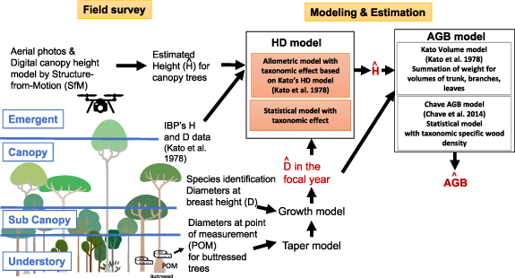
Figure 1. Methodological overview. Combined with field survey, drone survey and modeling, we obtained estimated diameter (D), height (H), and aboveground biomass (AGB) per tree.
Download figure:
Standard image High-resolution imageThis study was conducted in Pasoh Forest Reserve in Malaysia, where to date AGB and species diversity studies have been intensively conducted (Kato et al 1978, Hoshizaki et al 2004, Niiyama et al 2010, Okuda et al 2021). These previous study findings allowed us to compare and validate the results.
2. Materials and methods
2.1. Study sites and field survey
Our field survey was conducted in Pasoh Forest Reserve, Negeri Sembilan, Malaysia (2°59'N, 102°18'E, altitude 75–150 m, figure 2(a)). The average annual rainfall and temperature over 15 years (1997–2011) were 1 833 mm and 25.4 °C, respectively (Noguchi et al 2016). The vegetation type is lowland mixed dipterocarp forest, which is a common forest type in Malaysia, and the families Euphorbiaceae and Dipterocarpaceae are the two most abundant families represented in species among the number of individuals throughout the forest (Symington 1943, Wyatt-Smith 1961, 1964). We used a 6 ha plot within Pasoh Forest Reserve (figure 2(b)), which was established in 1994, and all living trees with a stem diameter at breast height (D) ⩾5 cm were tagged and identified at the species level, with a census every 2 years (Niiyama et al 2003). The center of the plot (2 ha, Plot 1) was used extensively for studies of primary productivity of tropical forests during the International Biological Program (IBP) in the 1970s (Kira 1978). Furthermore, the plot contains one flux tower (H 52 m), two canopy towers (H 30 m), and walkway between these towers.
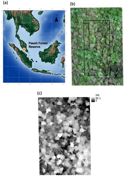
Figure 2. (a) A map of Pasoh Forest Reserve in Peninsular Malaysia. (b) An orthophoto mosaic of a 6 ha plot (200 m × 300 m) captured by a UAV, which includes the triangle canopy walkway in the right bottom, tower A in the right (with a height of approximately 52 m), tower B in the bottom (with a height of approximately 30 m), and the center rectangle is Plot 1 (100 × 200 m); the inner rectangle is the clear cut area (20 × 100 m) during IBP. (c) The Digital Canopy Height Model (DCHM) of the same 6 ha plot.
Download figure:
Standard image High-resolution imageHere, we conducted two types of field surveys in the 6 ha plot. The first is the survey of tree growth and survival conducted from 27 January–5 February in 2016 and 31 January–7 February in 2018. For buttressed trees, note that D was corrected using a taper model, and then D was estimated in September 2017 using a growth model (figure 1, supplementary text 1) to adjust the size of D and H in Sept 2017 for subsequent modeling analysis. The dataset included a total of 8150 individuals belonging to 72 families, 406 genera, and 570 species including 18 unidentified species and two individuals from unknown families (dataset S1). The second is a terrain survey to obtain topographic information of the plot; we conducted traverse measurement by measuring the distance, altitude difference, and direction using a laser range finder (Truepulse 200, Laser Technology Inc., Centennial, Colorado, USA) and a compass glass (Syakujii Keiki Co. Ltd, Tokyo, Japan) at each 10 m grid of the plot. Then, we obtained an averaged topographic map.
2.2. UAV survey and orthomosaic images and Digital Surface Model (DSM)
We conducted drone flights on 9 September, 2017, using a custom-made UAV (Hornbill Surveys, Sabah, Malaysia), which was controlled by autopilot software and mounted with a RedEdge camera (MicaSense, Inc., Seattle, WA, USA) equipped with a multispectral sensor capturing red, green, blue, near-infrared, and red-edge wavelengths and GPS (supplementary text 2). From the RGB images which constitute red, green, and blue colors captured by the camera, we created orthomosaic images and developed three-dimensional canopy models (DSM) using PhotoScan Professional, version 1.2.6 (Agisoft, St. Petersburg, Russia, www.agisoft.com). The detailed method is described in supplementary text 3.
2.3. Geographic information system (GIS) analysis
2.3.1. Digital Elevation Model (DEM) and DCHM
The DEM of the 6 ha plot was constructed based on the relative heights measured by a traverse method at 10 m grid size, and global navigation satellite system coordination of four peripherical points of the plot. The DCHM was calculated by the difference between DEM and DSM, which was produced by photogrammetry with PhotoScan. The total of 0.75% of the area with negative values in the DCHM was changed to zero, as it may be due to the error in the DSM or DEM. All GIS analyses were conducted using ArcMap 10.6.1 (ESRI, Redlands, California, USA).
2.3.2. Canopy identification and H estimation
To associate the canopy location with the tree ID in the field, we utilized canopy segmentation techniques that combine shape information from the DSM and RGB color data from the orthomosaic image (supplementary text 4, figure S2, Lim et al 2015). Overall, tree canopies were identified for 435 individuals in the 6 ha plot, comprising 42 families, 95 genera, and 146 spp., excluding Unknown (figure S2(b)). For these trees, the canopy heights were calculated as follows. First, we created 12 random points over each segmentation of the canopy. Then, we selected the 5 highest points per individual and calculated their mean. Here, because visible trees were mostly taller trees, thus the dataset for the smaller/shorter trees was not that abundant among the successfully identified canopies. Because those data of smaller trees would be necessary for robust estimation of the HD relationship, we added the IBP dataset, which was obtained by Kato et al (1978); these data contained the observed values of H and D for 156 trees in total, although not all the trees were identified in the species (dataset S2). Only 48 trees (30%) were identified at least by the family level, which consisted of 23 families, 35 genera, and 35 spp. For cases in which we did not know the taxonomic level, we considered the taxonomy as 'Unknown' and treated that data as one taxonomic class in the subsequent modeling analysis.
2.4. Development of the HD models
(1) Allometric model for HD relationship
The expanded allometric model by Ogawa et al (1965) is expressed as:
where H is a tree height, D is the diameter at breast height, a, h and  are coefficients. In particular, h is an allometric scaling exponent of HD growth and
  is the maximum tree height (Ogawa et al
1965, Kira and Ogawa 1971). Here, this model was termed MO (table S1). In a previous study (Kato et al
1978), MO was fitted to the empirical data of Plot 1 (within the 6 ha plot) in Pasoh Forest Reserve. The estimated parameters were a = 2, h = 1,
is the maximum tree height (Ogawa et al
1965, Kira and Ogawa 1971). Here, this model was termed MO (table S1). In a previous study (Kato et al
1978), MO was fitted to the empirical data of Plot 1 (within the 6 ha plot) in Pasoh Forest Reserve. The estimated parameters were a = 2, h = 1,  = 61, which assumed that all species or individuals had the same parameters. We refer to this as the Kato HD model. In this study, we incorporated the taxonomic effect into the parameters of this model. In addition, we treated the error associated with the year (or the type) of the dataset (6 ha, IBP) as random effects. Thus, the full model is described as follows:

where  ,
,  and
and  are the parameters nested with the taxonomic levels s of individual i, and is the error terms of the dataset as the year that the individual i was observed, respectively. We considered the taxonomic level of family and/or genus nested with family for the combination of three parameters of the model (table 1), which were eight models in total. Here, MO-0 was the conventional model of MO, which did not incorporate any effects.
Table 1. Summary of HD modelsaaa.
| Model type | Model no. | Equation | Parameters | Error | Taxonomic effect | LOOIC Statistics (SE) | Explained variation R2 (Error) | Coefficients | ||||||||||
|---|---|---|---|---|---|---|---|---|---|---|---|---|---|---|---|---|---|---|
| log Hmax | log a | h | ||||||||||||||||
| Mean | Q2.5 | Q97.5 | mean | Q2.5 | Q97.5 | Mean | Q2.5 | Q97.5 | ||||||||||
| Ogawa allometric model | MO-0 |

| a, h, Hmax | −432.2 | −39.8 | 0.89 | −0.003 | 4.387 | 4.229 | 4.583 | 0.916 | 0.791 | 1.037 | 0.824 | 0.76 | 0.889 | ||
| 1 |

| a, h, Hmax | year | −432.2 | −39.8 | 0.89 | −0.003 | 4.391 | 4.019 | 4.774 | 0.919 | 0.567 | 1.276 | 0.824 | 0.76 | 0.89 | ||
| 2 | a, h, Hmax | year | a, h, Hmax ∼ family | −436.8 | −42.1 | 0.9 | −0.003 | 4.352 | 2.668 | 6.028 | 0.914 | −0.783 | 2.589 | 0.835 | 0.75 | 0.921 | ||
| 3 | a, h, Hmax | year | Hmax ∼ family | −437.4 | −41.9 | 0.9 | −0.003 | 4.318 | 2.809 | 5.946 | 0.842 | −0.688 | 2.48 | 0.873 | 0.797 | 0.949 | ||
| 4 | a, h, Hmax | year | h, Hmax ∼ family | −436.6 | −42.2 | 0.9 | −0.003 | 4.269 | 2.341 | 5.891 | 0.8 | −1.16 | 2.403 | 0.864 | 0.789 | 0.938 | ||
| 5 | a, h, Hmax | year | a, h, Hmax ∼ family/genus | −437.6 | −42.1 | 0.9 | −0.004 | 4.323 | 2.425 | 6.167 | 0.942 | −0.974 | 2.778 | 0.828 | 0.742 | 0.917 | ||
| 6 | a, h, Hmax | year | Hmax ∼ family/genus | −438 | −41.9 | 0.9 | −0.003 | 4.295 | 2.605 | 6.087 | 0.831 | −0.856 | 2.623 | 0.876 | 0.8 | 0.952 | ||
| 7 | a, h, Hmax | year | h, Hmax ∼ family/genus | −436.8 | −42.2 | 0.9 | −0.003 | 4.23 | 2.232 | 5.816 | 0.785 | −1.225 | 2.38 | 0.868 | 0.794 | 0.943 | ||
| β0 | β1 | β2 | ||||||||||||||||
| mean | Q2.5 | Q97.5 | mean | Q2.5 | Q97.5 | mean | Q2.5 | Q97.5 | ||||||||||
| Statistical models | MS1-0 |

| β0 , β1 | −365.5 | −37.1 | 0.882 | −0.003 | 1.319 | 1.26 | 1.377 | 0.568 | 0.552 | 0.585 | |||||
| 1 |

| β0 , β1 | year | −364.4 | −36.5 | 0.882 | −0.003 | −1.184 | −3.413 | 1.352 | 0.56 | 0.538 | 0.582 | |||||
| 2 | β0 , β1 | year | β0 ∼ family | −382.4 | −37.8 | 0.888 | −0.003 | −1.146 | −3.364 | 1.447 | 0.536 | 0.51 | 0.562 | |||||
| 3 | β0 , β1 | year | β0 , β1 ∼ family | −433.5 | −39.3 | 0.9 | −0.003 | −1.013 | −3.195 | 1.568 | 0.496 | 0.449 | 0.539 | |||||
| 4 | β0 , β1 | year | β0 ∼ family/genus | −383.9 | −37.3 | 0.891 | −0.004 | −1.143 | −3.338 | 1.426 | 0.536 | 0.511 | 0.562 | |||||
| 5 | β0 , β1 | year | β0 , β1 ∼ family/genus | −449.5 | −38 | 0.909 | −0.004 | −0.987 | −3.187 | 1.63 | 0.479 | 0.436 | 0.521 | |||||
| MS2-0 |

| β0 , β1 , β2 | −433.1 | −39.6 | 0.894 | −0.003 | 0.677 | 0.517 | 0.835 | 1.012 | 0.908 | 1.115 | −0.07 | −0.087 | −0.054 | |||
| 1 |

| β0 , β1 , β2 | year | −435 | −41.1 | 0.895 | −0.003 | −1.982 | −4.219 | 0.565 | 1.065 | 0.948 | 1.182 | −0.076 | −0.094 | −0.059 | ||
| 2 | β0 , β1 , β2 | year | β0 ∼ family | −438.9 | −41.7 | 0.898 | −0.003 | −1.965 | −4.192 | 0.589 | 1.052 | 0.927 | 1.175 | −0.076 | −0.094 | −0.058 | ||
| 3 | β0 , β1 , β2 | year | β0 , β1 , β2 ∼ family | −437.5 | −41.6 | 0.899 | −0.003 | −1.788 | −4.004 | 0.765 | 0.964 | 0.724 | 1.161 | −0.066 | −0.094 | −0.032 | ||
| 4 | β0 , β1 , β2 | year | β0 ∼ family/genus | −439.7 | −41.7 | 0.9 | −0.003 | −1.906 | −4.153 | 0.648 | 1.049 | 0.923 | 1.172 | −0.077 | −0.095 | −0.058 | ||
| 5 | β0 , β1 , β2 | year | β0 , β1 , β2 ∼ family/genus | −444.6 | −40.5 | 0.907 | −0.004 | −1.566 | −3.805 | 1.03 | 0.84 | 0.589 | 1.074 | −0.05 | −0.083 | −0.016 | ||
(2) Statistical model for HD models
In previous studies, HD relationships were often formed as based on a power-law function and a polynomial function (Niklas 1995, Chave et al 2014), such as:


where i is an individual ID, and  ,
,  , and
, and  were parameters of each model. These models were termed MS1 and MS2, respectively (table S1). Then, we consider the taxonomic effect as random slopes and/or intercepts for the HD relationship for individual i as follows:


where  are the parameters nested with the taxonomic levels s of individual i, and
  is the error terms of the dataset as the year that individual i was observed. We also considered the taxonomic level of family and genus nested with family as for random intercepts and/or random slopes (table 1). Thus, there were six models for each MS1 and MS2 in total. Here, MS1-0 and MS2-0 were the conventional statistical models, which did not incorporate any taxonomic effects.
For each model, the Bayesian regression analysis was performed using a function 'brm' of 'brms' package (Bürkner 2017) in R; we ran each model across 2 chains for 120 000 iterations with a burn-in period of 20 000, thinned every 10 steps with the default prior sets. The models were compared using the approximate LOOIC based on the posterior likelihoods. For the models with the lowest (best) LOOIC in each model, we estimated fixed effects (means and 95% credible intervals) from the posterior distributions for each predictor.
2.5. AGB estimation
To estimate the AGB of each tree, we performed the following procedure: First, we estimated H from the estimated D for all trees in the 6 ha plot using the best HD models in (1) and (2) in the former section. The best HD models included taxonomic effects at family and genus levels (refer section 3.2 for further details). Then, the AGB per tree was estimated using both (a) the Kato volume model and (b) the Chave AGB model (also see table S1) as follows:
(a) Kato volume model (allometric equation)
The allometric models for the AGB of tree stems, branches, and leaves were developed by Kato et al (1978) as follows:

where WS, WB, and WL denote the dry mass of stem, branches, and leaves, respectively. Thus, these can be calculated from the estimated values of D and H. The total AGB for each tree was calculated as summation as follows:

(b) Chave AGB model for the pantropic model
One of the most common equations for calculating AGB was developed by Chave et al (2014), which was based on the relationship between AGB and D, H, and wood density (WD):

where is  of species
  of individual
  . To calculate the AGB using this equation, we used the 'BIOMASS' package in R (Réjou-Méchain et al
2017). The WD of each tree from its taxonomy (species, genus, family) can be attributed to the global WD database (Chave et al
2009, Zanne et al
2009) and the function 'getWoodDensity' with the region specified ('SouthEastAsiaTrop'). In the database, the mean WD values were available for 301 of 570 species (53%) at the species level, while at the genus level WD values were available for 240 species (42%). For the remaining four species and the unknown species (5%), the mean WD of the overall dataset was used. All AGB values for each tree were calculated using the 'computeAGB' function.
. To calculate the AGB using this equation, we used the 'BIOMASS' package in R (Réjou-Méchain et al
2017). The WD of each tree from its taxonomy (species, genus, family) can be attributed to the global WD database (Chave et al
2009, Zanne et al
2009) and the function 'getWoodDensity' with the region specified ('SouthEastAsiaTrop'). In the database, the mean WD values were available for 301 of 570 species (53%) at the species level, while at the genus level WD values were available for 240 species (42%). For the remaining four species and the unknown species (5%), the mean WD of the overall dataset was used. All AGB values for each tree were calculated using the 'computeAGB' function.
With these approaches for H and AGB estimation, we obtained four types of estimates of AGB, as a combination of two HD models—best models in (1) or (2) × one AGB model (Kato volume model or Chave AGB model). The AGB and D relationships were described at the family/genus level to assess the taxonomic difference. We also estimated AGB for all the trees in the 6 ha plot, and the total AGB was calculated as a summation of those.
2.6. Vertical distribution of AGB and species diversity layer
The vertical distribution of AGB and species diversity in the stratification of the forest structure were calculated as follows: all trees were classified into four stratification layer categories by estimated H (Sakai et al 1999), forest understory (⩽12.5 m), subcanopy (12.5–27.5 m), canopy (27.5–42.5 m), and emergent (>42.5 m) layers. We calculated the AGB and species diversity in each layer category, based on the estimated tree heights by the best HD models above. For species diversity, we used Hill numbers (Hill 1973) of order q = 0, 1, and 2, which are species richness, the exponential of Shannon index, and the inverse Simpson index, respectively. We also calculated Hill number-based functional diversity using by the package, 'mFD' in R (Magneville et al 2022). To calculate functional diversity, we used three functional traits: maximum D, mean WD, and number of the trees in the plot. Here, species diversity and functional diversity indices of q = 0, which do not incorporate species abundance, are mainly influenced by the number of rare species, whereas those of q = 1 and q = 2, which incorporate species abundance, are mainly influenced by these dominant species.
3. Results
3.1. H estimation for the HD model from DCHM
Based on the DCHM (figure 2(c)), we estimated the H of 435 trees with a mean (±SD) 33.2 ± 9.5 m. The tallest tree in the 6 ha plot was Koompassia malaccensis (55.6 m), followed by Shorea pauciflora (54.8 m), K. malaccensis (54.7 m), and Dipterocarpus cornutus (54.2 m, 53.7 m). The trees H >50 m were 14 trees in total in the 6 ha plot. The mean H (±SD) of the IBP dataset was 18.0 ± 11.3 m (N = 156). The IBP dataset also contained a direct measure of AGB (N = 156) (dataset S2).
3.2. HD models
According to LOOIC, the best models for the model types of MO and MS were MO-6 and MS1-5 (table 1, figures S3 and S4), respectively, for which both included taxonomic effects into family and genus levels. The selected models were better fitted than the conventional models—Ogawa allometric model (MO-0) and the two statistical models (MS1-0, MS2-0). Subsequently, we also calculated the root mean squared error (RMSE) of MO-6, MS1-5, MO-0, MS1-0, MS2-0 and Kato HD model, which were 4.42, 4.26, 4.60, 5.16, 4.61, and 5.00, respectively. Among all the models, the MS1-5 had the lowest LOOIC and the lowest RMSE, which indicated the model most fitted to the data.
Although the estimated H of the six HD models (MO-6, MS1-5, MO-0, MS1-0, MS2-0, and Kato HD model) did not differ in the smaller trees at the D approximately <75 cm, the difference of the estimated H increased as the D increased (at the D approximately >75 cm) (figure 3(a)). In both MO-6 and MS1-5, we found that the HD relationships differed among families and genera level (figures 3(b)–(e)). For example, in Dipterocarpaceae, the genera Dipterocarpus and Shorea were the tallest and second tallest among the genera in both MO-6 and MS1-5 (figures 3(b) and (e)). In Euphorbiaceae, Elateriospermum was the tallest genus in both models (figures 3(c) and (f)). Comparing to MO-6, MS1-5 showed more variation among genera in estimated H in smaller trees (D approximately <25 cm, figure 3(f)) because the  varied among genera (figure S4(b)). Likewise, in Fabaceae, MS1-5 exhibited more different patterns among genera than MO-6 (figures 3(d) and (g)). Both models predicted that the genus Koompassia was the tallest tree among the genera at the given D at a larger size (approximately >75 cm), while it was shorter than other genera at the given D at a smaller size (approximately <75 cm).
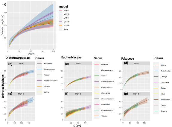
Figure 3. The height–diameter (HD) relationships estimated by allometric and statistical models. The solid line is the mean for the estimates. The surrounding polygon ribbon is the 95% credible interval estimated by 2000 predicted draws using the 'predicted_draws' function of the 'tidybayese' package. In (a), colors indicate the HD models used. In (b)–(g), relationships are shown for specific families/genera, with colors indicating genera in Dipterocarpaceae (b), (e), Euphorbiaceae (c), (f), and Fabaceae (d), (g). The HD models used are MO-6 (b)–(d) and MS1-5 (e)–(g).
Download figure:
Standard image High-resolution image3.3. AGB per tree and total AGB
3.3.1. Relationship between AGB and D
The relationships between the estimated AGB and D were similar in smaller trees but became different in larger trees as D increased among the four approaches of AGB estimation based on the best HD models in (1) MO-6 and (2) MS1-5 × two AGB models (Kato volume model or Chave AGB model) (figure 4(a)). Generally, the estimated AGB was higher in MS1-5 than that in MO-6, and higher in the Chave AGB model than that in the Kato volume model. The choice of HD model resulted in a greater difference in AGB estimation than the choice of AGB model. Moreover, the difference became larger with a larger D (approximately 150 cm). The RMSE values for the directed measures of AGB in IBP (N = 156, Kato et al 1978) were 0.537, 0.389, 0.448, and 0.306 for the MO-6 × Kato model, MS1-5 × Kato HD model, MO-6 × Chave AGB model, and MS1-5 × Chave AGB model, respectively.
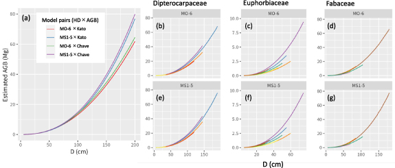
Figure 4. The aboveground biomass–diameter (AGB-D) relationships estimated by selected HD models × AGB models. The solid line is the mean for AGB estimates. The surrounding polygon ribbon is the 95% credible interval, which was derived by H estimation using the same method in figure 3 (although it is too small to see in the figure). In (a), colors indicate the pairs of height–diameter (HD) models and AGB models. In (b)–(g), relationships are shown for specific families/genera, with colors indicating genera in Dipterocarpaceae (b), (e), Euphorbiaceae (c), (f), and Fabaceae (d), (g), as in figure 3. The HD models used are MO-6 (b)–(d) and MS1-5 (e)–(g), and the AGB model was the Chave AGB model.
Download figure:
Standard image High-resolution imageWe also explored the taxonomic difference in the relationship between the estimated AGB and H (MO-6 or MS1-5 and Chave AGB model). The estimated AGB varied among families and genera in both the MO-6 and MS1-5 models (figures 4(b)–(g)). In Dipterocarpaceae (figures 4(b) and (f)), the genera Dipterocarpus and Neobalanocarpus had higher AGB at given D than Shorea; for example, Dipterocarpus had about 1.8-fold AGB compared with the genus Shorea in a 100 cm D tree. In Euphorbiaceae (figures 4(c) and (g)), the genus Elateriospermum had the highest AGB at given D, and in Fabaceae (figures 4(d) and (f)), the genus Koompassia had the highest AGB at a given D.
3.3.2. Total AGB in Pasoh Forest Reserve
The estimated total AGB in the 6 ha plot by the best HD models, the MO-6 and MS1-5, × the Chave AGB model was 503.2 and 518.3 Mg ha−1, respectively (table 2). These estimates fell within the ranges obtained using conventional methods, which were 457.6–534.4 Mg ha−1. Overall, for the AGB models, the estimates based on the Chave AGB model were larger than those based on the Kato volume model. However, regarding the HD model, the estimates based on MS1-5 were larger than those based on MO-6, whereas the difference between the two HD models was not large compared with the differences among AGB models. Regarding families, Dipterocarpaceae most contributed to the total AGB, about 42% according to the estimates by both best HD models × Chave AGB model (figure S5). The second and third contributing families were Fabaceae and Euphorbiaceae, which were about 12% and 6% of the total AGB, respectively.
Table 2. Comparison of AGB estimates in Pasoh Forest Reserve. In the 'Area' column, the designations A, C, P1–P4 correspond to areas outside of the 6 ha plot and are defined in each reference.
| Forest type | Area | Year | HD model | AGB model | AGB (Mg ha−1) | Reference |
|---|---|---|---|---|---|---|
| Primary forest | 6 ha plot | 2017 | MO-6 | Kato | 457.6 | This study |
| MS1-5 | Kato | 470.8 | ||||
| MO-6 | Chave | 503.2 | ||||
| MS1-5 | Chave | 518.3 | ||||
| Kato | Kato | 475.8 | ||||
| MS1-0 | Chave | 534.4 | ||||
| MS2-0 | Chave | 508.2 | ||||
| Logged forest | C | 1998 | Kato | Kato | 261 | Okuda et al 2021 |
| 2012 | Kato | Kato | 315 | |||
| Primary forest | 6 ha plot | 1994–2006 | Kato | Kato | 363 | |
| A (50 ha) | Kato | Kato | 310 | |||
| Primary forest | P1 | Kato | Kato | 542 | Niiyama et al 2010 | |
| P2 | Kato | Kato | 648 | |||
| P3 | Kato | Kato | 436 | |||
| P4 | Kato | Kato | 519 | |||
| Primary forest | 6 ha plot | 1998 | Kato | Kato | 431.2 | Hoshizaki et al 2004 |
| Kato | Kato | 403 | ||||
| Primary forest | A part of 6 ha (Plot 1) | 1971 | Kato | Kato | 664.0 | Kato et al 1978 |
| A part of 6 ha (Plot 2, DBH >4.5 cm) | 1973 | Kato | Kato | 475.2 |
3.4. Vertical distribution of AGB, species diversity, and functional diversity
The vertical patterns of AGB, which was estimated by both the best HD models × Chave AGB model, number of individuals, species diversity, and functional diversity were described in figure 5; we found that the vertical patterns were contrasting among indices. AGB increased along with the layer. The emergent layers held the highest AGB, 44% of the total AGB (figures 5(a) and (b)). In this layer, Dipterocarpaceae followed by Fabaceae were the major components of the total AGB in the emergent layer, at ∼62% and ∼21%, respectively. In the canopy layer, Dipterocarpaceae followed by Euphorbiaceae and Fabaceae contributed to the total AGB in the layer, at 36%, 9% and 7%, respectively. In contrast, in the subcanopy and understory layers, these dominant families shared less in the total AGB; for example, Dipterocarpaceae contributed only ∼12% of the total AGB, and families other than Dipterocarpaceae, Euphorbiaceae, and Fabaceae comprised ∼74% of the total AGB in the subcanopy and understory layers. The total number of individuals was higher in the lower, subcanopy, and understory layers. In particular, the most abundant family regarding the number of individuals in the subcanopy and the understory layer was Euphorbiaceae, at 13% and 16%, respectively. Likewise, the indices on species diversity decreased along with the layer; lower layers held higher species diversity (figures 5(d)–(f)). In particular, the species richness of Dipterocarpaceae, Euphorbiaceae, and Fabaceae, which were the major sources of AGB, were only a small part of the total species richness in the understory layer, at 6%, 6%, and 3%, respectively. Among the functional diversity indices, the functional diversity of q = 0 was highest in the understory layer, whereas the functional diversity of q = 1 and q = 2 were highest in the canopy layer (figures 5(h) and (i)).

Figure 5. The vertical distribution of aboveground biomass (AGB) and species diversity indices across four layers: forest understory (<12.5 m, US), subcanopy (12.5–27.5 m, SC), canopy (27.5–42.5 m, C), and emergent (>42.5 m, E). Each panel displays a different metric: (a) AGB (Mg ha−1) based on the MO-6 × Chave AGB model, (b) AGB (Mg ha−1) based on the MS1-5 × Chave AGB model, (c) number of individuals (trees ha−1), (d) species richness (Hill number q = 0), (e) exponential Shannon index (Hill number q = 1), (f) inverse Simpson index (Hill number q = 2), (g) functional diversity (FD) (Hill number q = 0), (h) FD (Hill number q = 1), and (i) FD (Hill number q = 2). In panels (a)–(d), color indicates the families. Tree height was estimated based on (b) MS1-5, otherwise MO-6.
Download figure:
Standard image High-resolution image
4. Discussion
4.1. HD relationship
This study showed that HD models formulated by relating H against not only D but also taxonomic effect best performed statistically. This finding indicates the importance of taxonomic-specific HD for accurate estimation of H. The HD relationships varied more in genus level than in family level; in particular, we found higher variation even in smaller trees in the genera of Euphorbiaceae and Fabaceae. This finding may be attributed to these families that consist of species with higher interspecific trait variation; for example, Euphorbiaceae holds both light-demanding species, such as the genus Macaranga, and shade-tolerant species, such as the genus Elateriospermum. These growth trait variations are also linked with WD or carbon accumulation efficiency—for example, fast-growing trees generally have low WD, whereas slow-growing trees exhibit the opposite. Fabaceae holds not only subcanopy or canopy species but also emergent tree species (i.e., the genus Koompassia), which can be the highest at a given D approximately >110 cm. In contrast, Dipterocarpaceae showed more similar HD relationships among genera, especially in smaller trees. Because dipterocarp are generally shade-tolerant and slow-growing species (Manokaran and Kochummen 1994, Köhler et al 2000), we found similar patterns of the HD relationship among the genera in the forest floor. However, some species in the genus Shorea (i.e., light red meranti), have a relatively higher growth rate compared with the other dipterocarp species, especially under the fine light conditions (Takeuchi et al 2005), which suggests that we might underestimate the variation in the HD relationship within the genus. The differences in traits and life-history strategies among species can lead to variations in HD relationships, even within the same taxonomic group. Furthermore, these HD relationships predict a H threshold where H cannot increase beyond a certain point despite an increase in D. This relationship implies that the HD model can partially indicate the growth strategies of different taxonomic groups, including whether they grow vertically (H) or horizontally (D), based on their age and size. Our results also revealed potentially the highest genus groups in the forest in the largest D-size class—the genus Dipterocarpus of Dipterocarpaceae and Koompassia of Fabaceae. In fact, these were ranked in the top ten highest trees in the 6 ha plot. In contrast, this study was missing the species-level effect. Here again, for example, S. pauciflora was also the tallest tree in the plot. Because Shorea at the genus level was not estimated to be high enough, we overlooked the effect. Therefore, the species-level model requires further study.
4.2. AGB estimation
Accurate prediction of H is crucial for improving the estimation of AGB (Kearsley et al 2017). This study showed that the HD models developed at the taxonomic level better fit the AGB-D relationship statistically. The logarithmic relationship between AGB and D indicates that larger trees make a bigger contribution to the total AGB. The AGB-D relationships varied among genera, and the study revealed which genera had higher AGB for a given D. For example, larger trees in the genera Dipterocarpus, Neobalanocarpus (Dipterocarpaceae), Elateriospermum (Euphorbiaceae), and Koompassia (Fabaceae) are likely significant contributors to AGB storage in the forest.
The total estimated AGB in Pasoh Forest Reserve varied among the different AGB models. However, no significant differences were observed between the HD models. This finding may be because most of the trees in the 6 ha plot were small, and the AGB-D relationships were similar among MO-6 and MS1-5 for smaller trees. The larger difference between the Chave AGB model and Kato model highlights the crucial role that taxonomy plays in the AGB models because the Chave model includes taxonomy-specific WD. Larger AGB estimated by the Chave AGB model suggested a high abundance of species with larger WD, which resulted in about 10% higher than that estimated by the Kato AGB model. Thus, these findings indicate that AGB estimation without the taxonomic effect would lead to underestimation of the total AGB in the tropical forest. In fact, even the minimum estimate in our results in 2017, which was 457.5 Mg ha−1, was higher than that in the previous estimates in 1998 (431.2 Mg ha−1, Hoshizaki et al 2004). This would be also resulted from the growth of the forest. The estimated total AGB in 2017 in the comparable (conventional) method was 475.8 Mg ha−1, which was far higher than that in the previous report, which indicated that AGB increased at by an average of 2.3 Mg ha−1 per year in 1998–2017. The total AGB of tropical forests generally highly fluctuated with time, as well as space (Okuda et al 2021). In particular, because the plot included a 'disturbed area' in the past; these areas would have recovered in more recent years and contributed to increased AGB, which was also suggested in the former study (Okuda et al 2021).
Previous studies have highlighted the importance of developing local HD models for accurately estimating AGB in tropical forests (Feldpausch et al 2012). This is primarily because HD relationships can vary across continents, regions, forest types, and taxonomic compositions (Banin et al 2012). Utilizing a local HD model can help minimize error in AGB estimation, even when generalized pantropical AGB models are used (Chave et al 2014, Popkin 2015, Kearsley et al 2017, Fayolle et al 2018).
Similarly, AGB models can be site-specific. Several allometric AGB models have been developed for Southeast Asian tropical forests across different sites (Kato et al 1978, Yamakura et al 1986, Ketterings et al 2001) and forest types (Pinard and Cropper 2000, Kenzo et al 2009). This study employed a generalized pantropical AGB model with a species-specific variable, WD, to account for site-specificity in terms of species composition. Although this study developed a local HD model by considering tree taxonomic groups and contributed to the improvement of subsequent AGB models, further enhancements to the AGB model remain a future challenge. It has been suggested that incorporating taxonomic-based estimation can enhance the performance of AGB models (Basuki et al 2009, Paul et al 2016).
4.3. Vertical patterns of AGB and species diversity
The study of AGB and biodiversity patterns in Pasoh Forest Reserve using HD and AGB models, including the taxonomic effect, helped to develop an understanding of the role of taxonomy in determining the total AGB and its vertical distribution. The major families contributing to the total AGB were Dipterocarpaceae, Euphorbiaceae and Fabaceae, mostly from trees in the emergent and canopy layers. This finding is consistent with previous studies that showed that large trees have a significant impact on the total AGB of tropical and temperate forests (Lutz et al 2012, 2018, Slik et al 2013, Fayolle et al 2018, Fotis et al 2018). In contrast, species diversity was higher in the lower layers of the forest. This contrasting pattern suggests that the mechanisms governing species diversity are different in the canopy and understory layers (Mensah et al 2018). The canopy layer, occupied by a limited number of tree species, is responsible for storing AGB. This pattern can be explained by the selection effect (Fox 2005, Fotis et al 2018). The understory layer has a high number of individuals with diverse species coexisting in heterogeneous local environments, which is consistent with the niche differentiation effect (Brown et al 2013, Johnson et al 2017). It suggests that a taller canopy promotes the species coexistence by producing the heterogeneous local environments under light conditions and moisture availability caused by canopy openings in the emergent and canopy layers (Wright et al 2010). In addition, trees in the understory and the subcanopy layer would contribute to forest productivity more than taller trees in a tropical forest (Kohyama et al 2023). Moreover, species diversity in the understory is a source of potential carbon sources for future large trees. Therefore, interaction and differences in the governing mechanism between the canopy and understory would be essential for both high AGB and high species diversity in the forest.
This study also found the higher functional diversity in the upper middle layers, which is more similar to that of AGB rather than that of species diversity. Functional diversity is more closely related to ecosystem processes and dynamics and would have a stronger predictive power for AGB than species diversity (Ruiz-Benito et al 2014, Tobner et al 2016). Thus, functional diversity could be a potential indicator of ecosystem functioning in forest stratification (Dıéaz and Cabido 2001, Cadotte et al 2011) although species richness and functional diversity are often correlated (Tobner et al 2016).
5. Conclusion
In summary, this study highlights that taxonomic consideration can improve the models for the HD relationship and consequent AGB estimation in tropical forests. The study found that specific families, such as Dipterocarpaceae, Euphorbiaceae, and Fabaceae were major contributors to the total AGB in the forest and were mainly found in the emergent and canopy layers. Thus, to maintain high AGB in the forest, large trees of those families could be the target for conservation in terms of carbon storage. As such, the identification of key taxonomy for forest stratification and AGB would be helpful for effective forest management to identify the conservation target and silvicultural targets in terms of protection and restoration of the carbon source (Lindenmayer et al 2014).
The study also found that, whereas the canopy layers had fewer species and most of the AGB, understory trees play a crucial role in species diversity, which is also linked to essential ecosystem processes such as forest regeneration, nutrient cycling, and plant–animal interaction (Nilsson and Wardle 2005). The relationship between biomass and diversity in forests is strongly influenced by the vertical structure of the forest. Understanding this relationship and the underlying mechanisms is crucial for forest management and conservation. Finally, the study used a drone to measure H, and advancements in airborne laser scanning technology (Asner et al 2014, Asner and Mascaro 2014, Kent et al 2015, Chan et al 2021) can now be used to measure H even in the understory layers, making forest monitoring more efficient and cost-effective.
Acknowledgments
We thank the members of the field station in Pasoh Forest Reserve for their kind support for the study. We profoundly thank Drs T Kira and T Yoneda for providing us the original census and sampling data obtained in the IBP project. We are also grateful to Dr M Onishi for his assistance in the field survey and GIS analysis. This study was conducted under the NIES/FRM/UPM projects. This study was financially supported by National Institute for Environmental Studies, partially supported by JSPS KAKENHI Grant Number 19H04323 and JST/JICA SATREPS (PUBS).
Data availability statements
The data that support the findings of this study are openly available at the following URL/DOI: https://doi.org/10.5281/zenodo.7866644. Additionally, Dataset S1 will be available on GBIF at https://gbif.jp/ipt/resource?r=nies_pasoh_trees after January 2024.
Conflict of interest
The authors have no competing interests to declare.
Supplementary data (2.0 MB PDF)