

Abstract
This article proposes an inverted U-shape relationship between air pollution and criminal behavior. Exposure increases criminality by raising criminals' taste for risk and violent behavior while also reducing it by changing the number of felons and crime opportunities in the market through exacerbated morbidity and avoidance behavior. I illustrate both mechanisms with an expected utility model of the decision to delict and a simplified search and matching frictions model between criminals and crime opportunities. Linear, quadratic, and nonparametric Poisson pseudo-maximum likelihood estimator panel models confirm this bell-shaped relationship for Mexico City and New York, suggesting that the linear association between pollution and criminality uncovered by late studies may be better estimated with nonlinear models.
Export citation and abstract BibTeX RIS

Original content from this work may be used under the terms of the Creative Commons Attribution 4.0 license. Any further distribution of this work must maintain attribution to the author(s) and the title of the work, journal citation and DOI.
1. Introduction
Although current studies on the effects of air pollution on criminal behavior provide convincing evidence of a linear and positive relationship between pollution and crime (e.g. Burkhardt et al 2019, Bondy et al 2020, Herrnstadt et al 2020) 3 , these studies mainly concentrate on exposure's linear effect, ignoring nonlinearities or treating them as mere robustness. In this paper, I provide evidence for nonlinear effects and show that ignoring them can lead to the wrong interpretation of linear coefficients.
The nonlinear relationship between pollution and crime emerges because of two conflicting mechanisms; the impact of exposure on the decision to transgress and on the matching of felons and crime opportunities. In a nutshell, although pollution increases the likelihood of committing a crime (e.g. Bondy et al 2020), it also affects the match of criminals and crime opportunities by reducing the number of agents in the market through exacerbated morbidity (e.g. Knittel et al 2016) and avoidance behavior (e.g. Moretti and Neidell 2011). I propose that the conflict between these two mechanisms leads to a nonlinear (inverse U-shaped) relationship between both variables.
Besides a more careful assessment of the functional form, I contribute to the ongoing literature on the relationship between criminality and air pollution in three ways. First, I develop a more nuanced theoretical foundation for the effects of pollution on the no-crime condition. Second, I assess if the previously estimated positive relationship holds at high-frequency intervals by using hourly data to examine the impact of pollution on criminality. Third, I provide the first estimates of the pollution-crime relationship for a city in the developing world (Mexico City)
4
 5
.
5
.
The data set for the estimation consists of 2.9 million hourly observations on the number of crimes, pollution levels, and weather conditions in the vicinity of pollution measuring stations in Mexico City and New York. To estimate the effect of pollution on crime, I use the now-cast air quality index (NowCast AQI) as a proxy for hourly exposure and assess its impact on criminality with high dimensional Poisson pseudo-maximum likelihood estimator (PPML) panel models.
Results show that air pollution increases criminality. Raising the NowCast AQI by ten units increases crime by 0.33% and 0.48% in Mexico City and New York. This higher linear estimate for New York suggests that exacerbated exposure may reduce Mexico City's linear coefficients through higher morbidity. I consider this by estimating quadratic and non-parametric panel models confirming that even though pollution increases crime at standard levels, the relationship reverses during episodes of exacerbated exposure. I complete the empirical section by showing that estimating the effect of pollution on crime with linear models can lead to the wrong interpretation of the pollution-crime relationship when looking at specific crime categories. Also, note that all results hold when using different control variables, samples, and estimators.
1.1. Related literature
The connection between air pollution and criminal behavior arises from pollution's effect on several physiological, psychological, and environmental factors. Air pollutants promote inflammatory responses and changes in the chemical composition of the central nervous system 6 , altering the brain's chemistry and leading to behavioral alterations like irritability, changes in risk preferences, and exacerbated eagerness for rewards. For example, there is epidemiological evidence that higher concentrations of air pollution can increase aggressive, impulsive, and overexcited behavior in animals (Petruzzi et al 1995, Chen et al 2003, Soulage et al 2004, Xu et al 2021), changes in risk attitudes for human beings (Heyes et al 2016, Bondy et al 2020), and affectations in the brain's level of serotonin (Murphy et al 2013); a chemical compound that works as an inhibitor of impulsive and aggressive behaviors. Moreover, exposure can also affect criminals' labor supply and crime opportunities through exacerbated morbidity and avoidance behavior (Tolbert et al 2000, Iskandar et al 2012, Knittel et al 2016).
The literature on the relationship between pollution and crime is continuously growing and expanding across different disciplines like psychology (Lu et al
2018, Younan et al
2018), epidemiology (Berman et al
2019), and health sciences (Mapou et al
2017). For economics, Herrnstadt et al (2020) uses the interaction between wind direction and micro-geographic information to show that violent crime is 1.9% higher downwind of interstate highways (a known source of air pollution) in Chicago. Bondy et al (2020) use PPML estimator panel models to estimate that increasing the AQI by ten units increases crimes by 1.7% in London. Burkhardt et al (2019) use fixed-effects panel models alongside American crime statistics to conclude that raising coarse particulate matter (PM10) and atmospheric ozone (O3) by ten percent increases violent crimes by 0.14% and 0.35% across a sample of US counties. Moreover, different from Bondy et al (2020) and Burkhardt et al (2019), Herrnstadt et al (2020)find no evidence of an effect of exposure on non-violent felonies. Finally, Chen and Li (2020) exploit the variation in the  Budget Trading program to show that violent and property crimes are 3.7% and 2.9% lower in states that participated in the emissions trading scheme.
2. Theoretical background
This section proposes a theoretical pathway for the relationship between pollution and crime. Equation (1) portrays the no-crime condition (Becker 1968). In it, p is the probability of apprehension, and U(x) is the utility function under prospect theory. U(x) depends on the income from committing ( ) and not-committing (
 ) the crime; the reference point from which criminals elicit their utility (y0); and the cost of apprehension (F). For simplification and without loss of generality, I assume that the income from not committing the crime (
 ) and the reference point for elicitation (y0) are equal to zero. Under these assumptions, equation (1) reduces to
  7
. In it, a person commits a crime if the utility of doing so is greater than zero
7
. In it, a person commits a crime if the utility of doing so is greater than zero

Previous literature on the relationship between pollution and crime assumed that exposure increases criminality by affecting the no-crime condition, i.e.  . This assumption rests on previous studies showing that exacerbated exposure can lead to higher eagerness for rewards, aggressive behavior, and taste for risk in humans and animals (e.g. Petruzzi et al
1995, Chen et al
2003, Soulage et al
2004). Now, assuming a felony occurs every time the no-crime condition for criminal c at time t is larger than zero. The total number of felonies for an entire region and period is a Poisson distributed count variable of the form:
. This assumption rests on previous studies showing that exacerbated exposure can lead to higher eagerness for rewards, aggressive behavior, and taste for risk in humans and animals (e.g. Petruzzi et al
1995, Chen et al
2003, Soulage et al
2004). Now, assuming a felony occurs every time the no-crime condition for criminal c at time t is larger than zero. The total number of felonies for an entire region and period is a Poisson distributed count variable of the form:

Figure 1 provides evidence of the suitability of the Poisson distribution for the count of crimes occurring around measuring stations in Mexico City and New York. In it, I plot the probability mass function of four simulated Poisson distributions with different λ values alongside the crime sample.

Figure 1. Probability mass function for different Poisson distributions.
Download figure:
Standard image High-resolution imageAn additional concern is that the realization of criminal activities is not only a function of the individual decision to commit a crime but also the environment where the crime takes place, e.g. even if a criminal's no-crime condition is higher than zero, it still requires particular market conditions like available crime opportunities before pursuing these activities. In this study, I propose that high morbidity reduces criminality by decreasing criminals' labor supply and crime opportunities in the market for criminal activities. For instance, Imagine a market where criminals (c) find victims (v) through the matching technology  in the spirit of Mortensen and Pissarides (1994).
  is concave, strictly increasing in both parameters, and exhibits constant returns to scale. Figure 2(a) shows the shape of this matching function, and figure 2(b) the theoretical relationship between air pollution and the count of victims and criminals in the market
8
. Form this figure, it follows that the number of agents and matches in the market decrease as air pollution increases, i.e.
is concave, strictly increasing in both parameters, and exhibits constant returns to scale. Figure 2(a) shows the shape of this matching function, and figure 2(b) the theoretical relationship between air pollution and the count of victims and criminals in the market
8
. Form this figure, it follows that the number of agents and matches in the market decrease as air pollution increases, i.e.  .
.
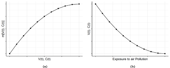
Figure 2. The matching function and the effects of pollution on market agents. (a) Relationship of the matching function with the number of victims and criminals. (b) Relationship between exposure to air pollution and the number of victims and criminals.
Download figure:
Standard image High-resolution imageFelons match with victims through the previously mentioned Poisson process of rate  . If we assume a Cobb–Douglas matching function of the form
  , where c is equivalent to the number of individuals eliciting a positive utility from criminal activities, i.e.
  , it is straightforward to show that the relationship between air pollution and the number of crimes in the market takes the following form:

In it, the total number of crimes (or matches) in region r at time t is a function of the exogenous technology parameter A, the number of criminals in the market  , and the amount of crime opportunities vrt
. Taking the logs of this function and assuming that
, and the amount of crime opportunities vrt
. Taking the logs of this function and assuming that  , its easy to show that the number of crimes at time t in region r depends on the count of active criminals in the market crt
, which is in turn a function of air pollution
, its easy to show that the number of crimes at time t in region r depends on the count of active criminals in the market crt
, which is in turn a function of air pollution  and other determinants of the no-crime condition (Xrt
). In the empirical section, I estimate the effect of
and other determinants of the no-crime condition (Xrt
). In the empirical section, I estimate the effect of  on Crimes
 while considering the potential bias arising from Xrt
according to:
while considering the potential bias arising from Xrt
according to:

Combining the insights of this section, I propose that, even though air pollution increases criminality at low-to-moderate exposure levels because of its effects on the no-crime condition (see Bondy et al 2020), the relationship between both variables reverses at high exposure intervals due to higher morbidity and avoidance behavior. The interaction between these two mechanisms leads to the proposed inverse U-shaped relationship.
This critical insight stands contrary to the monotonic and increasing relationship of late studies, where nonlinearities are only interesting in exploring the second derivative's steepness and assessing the shape of the dose-response function. Figure 3 provides some intuition for the proposed functional form. The effect of pollution on crime reaches its maximum at the level of pollution that maximizes criminality. Before this point, the impact of air pollution on the criminals' propensity to commit a crime is higher than its effect on avoidance and morbidity. After that, the morbidity channel becomes dominant and starts decreasing criminality.
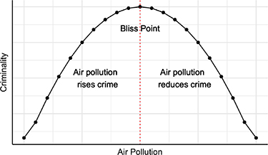
Figure 3. Theoretical relationship between air pollution and crime; the red line marks the level of air pollution that maximizes criminality, i.e.  .
.
Download figure:
Standard image High-resolution image3. Data
I obtain data on criminal activity from the open data portal websites of Mexico City and New York (City of New York 2020, Ciudad de Mexico 2020) 9 . Both data sets include the hour, date, place, and type of crime. Because of different crime classifications, I sort offenses into eight subgroups: homicide, aggravated assaults, non-aggravated assaults, robbery, burglary, larceny, sex crimes, and fraud 10 .
Figure 4 presents hourly, monthly, and yearly time series of criminality. The left panel shows higher crime numbers during the late evening hours and a significant midday peak in Mexico City. This increase could happen because of miss-recordings. I deal with this possible source of bias with fixed effects and robustness exercises where I exclude crimes happening at midday from the empirical strategy. In line with the relationship between heat and aggressive behavior (see Ranson 2014), monthly variation indicates higher crime numbers in the summer while long-term trends show a steep growth in the number of felonies for Mexico City alongside an apparent decline for New York.
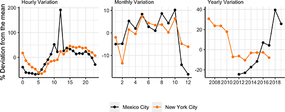
Figure 4. The grid shows the temporal behavior of criminality in Mexico City and New York. Clockwise it shows the hourly, monthly, and yearly variation concerning the average.
Download figure:
Standard image High-resolution imageAs is typical with empirical analyses of criminal behavior, the data only includes reported felonies. This issue is problematic for crimes like sexual offenses, where social stigmatization may discourage reporting. However, as long as reporting correlates with actual crimes, this issue should not affect empirical estimates. Another problem is that I only observe the pollution level in the vicinity of the crime. I deal with this source of measurement error by instrumenting air pollution with wind direction in the robustness section.
Air pollution data comes from the monitoring stations of the US Environmental Protection Agency 11 and the center for atmospheric information of Mexico City 12 . I obtain hourly measures of PM10, Fine Particulate Matter (PM25), and O3 for 25 stations in Mexico City and 27 in New York 13 . To obtain a single estimate of the effect of pollution on criminality, I convert the hourly concentration of O3, PM10, and PM25 into the NowCast AQI; an hourly version of the standard AQI that transforms the concentration of the main criteria pollutants into an index running between 0 and 500 units. Figure 5 shows the location of measuring stations in both cities.

Figure 5. Location of pollution measuring stations in Mexico City and New York.
Download figure:
Standard image High-resolution imageI construct the final data set by adding the number of hourly crimes happening in a 2 km radius around each measuring station. In cases when a crime falls within the catchment area of two different stations, I assign the crime to the closest one. However, results are robust to double counting and different catchment radii. The final data set is a panel of 2.9 million hourly observations 14 . Each observation contains the number of crimes occurring around each measuring station at time t alongside recorded pollution values and weather covariates.
Table 1 shows some descriptive statistics. In line with the count nature of the data, there is a significant share of observations with zero values alongside suggestive evidence of overdispersion (i.e.  ), an insight that I incorporate into the empirical methodology by estimating the relationship between pollution and crime with PPML estimators.
Table 1. Descriptive statistics on the number of hourly crimes happening in a 2 km radius around pollution measuring stations in Mexico City and New York.
| Obs period | Average | Variance | Min | Max | N | Zeros N | Zeros % | |
|---|---|---|---|---|---|---|---|---|
| Mexico City | ||||||||
| Total | 2012–2019 | 0.303 | 0.528 | 0 | 46 | 1433 832 | 1125 888 | 79 |
| Violent | 2012–2019 | 0.104 | 0.12 | 0 | 7 | 1433 832 | 1301 749 | 91 |
| Non violent | 2012–2019 | 0.100 | 0.154 | 0 | 21 | 1433 832 | 1316 376 | 92 |
| New York | ||||||||
| Total | 2006–2017 | 0.926 | 1.75 | 0 | 55 | 1510 319 | 785 423 | 52 |
| Violent | 2007–2017 | 0.163 | 0.219 | 0 | 11 | 1510 319 | 1311 999 | 87 |
| Non violent | 2007–2017 | 0.322 | 0.464 | 0 | 22 | 1510 319 | 1154 301 | 76 |
Weather data comes from 13 monitoring stations of the National Oceanic Atmospheric Administration, station-level information from the EPA, 13 measuring stations in Mexico City, and all stations reported in the Global Surface Summary of the Day of the USA National Centers for Environmental Information. I use temperature, rain, wind speed, and relative humidity as covariates and wind direction as an instrument.
4. Empirical design
The empirical strategy assesses the functional relationship between both variables with linear, quadratic, and nonparametric designs on the effects of air pollution on the number of crimes happening around pollution measuring stations in Mexico City and New York. Given the count nature of the data, heteroskedasticity, and a significant share of observations with zero values, I use PPML estimators (Silva and Tenreyro 2006, Wooldridge 2010) 15 . However, all results are robust to alternative estimators like negative binomial, ordinary least squares estimators (OLS), and log-linear OLS.
Equation (5) shows the primary estimation equation. In it, Cst
measures the number of crimes happening in a 2 km radius around station s at time t.  is the NowCast AQI and γ the point estimate of interest measuring the impact of an additional NowCast AQI unit on the log difference of crime counts. I consider the relationship between weather, pollution, and criminality with a flexible specification of temperature, precipitation, relative humidity, and wind speed—
 . Specifically, I account linearly for wind speed and relative humidity and nonparametrically for temperature and precipitation
16
. Specifically, I account linearly for wind speed and relative humidity and nonparametrically for temperature and precipitation
16

Year-by-month-by-station fixed-effects ( ) control for cross-sectional discrepancies between measuring stations arising from systematic differences in neighborhood characteristics and intra-year seasonality. Hour (
 ) and day of the week (
 ) fixed-effects control for unobservables affecting both crime and productivity at the hourly and weekday levels
17
.
) fixed-effects control for unobservables affecting both crime and productivity at the hourly and weekday levels
17
.
After estimating the linear effect of pollution on criminality, I assess the functional form with a quadratic version of equation (5). This quadratic model parametrically estimates the dose-response function by regressing the number of crimes around measuring stations on the linear and squared value of the NowCast AQI. If the quadratic model leads to a better fit (as measured by the Bayesian Information Criterion (BIC)) alongside positive linear and negative quadratic coefficients, equation (6) would provide parametric evidence of a nonlinear (inverse U-shaped) relationship between both variables

Once I assess the nonlinear relationship with the quadratic model, I estimate it nonparametrically by dividing the NowCast AQI into six self-contained exposure intervals and examining the effect of 1 h in each interval concerning the lowest exposure bin. Equation (7) shows the estimation design of the nonparametric PPML model. In it,  is a dummy vector equal to one when the NowCast AQI in station s at time t falls in bin b

5. Results
Table 2 presents the results of three different specifications for the effect of the NowCast AQI on the number of crimes happening in Mexico City and New York. All specifications contain weather controls and only vary in their fixed effects. (a) Controls for station, month, hour, and weekday fixed effects, (b) accounts for seasonality by including an interaction term of year-by-month fixed effects, and (c) further interacts year-by-month with station fixed effects. The third design is the preferred specification as it identifies air pollution's impact on criminality from within-month variation across measuring stations. To simplify the interpretation of coefficients, I transform the value of β to ![$[\mathrm {exp}(\beta) -1] \times 1000$](https://content.cld.iop.org/journals/2752-5309/1/2/021001/revision4/erhac9a65ieqn28.gif) and interpret it as the percentage increase in criminality because of ten additional NowCast AQIs.
and interpret it as the percentage increase in criminality because of ten additional NowCast AQIs.
Table 2. Effect of pollution on criminality (linear model).
| Mexico City | New York | |||||
|---|---|---|---|---|---|---|
| (1) | (2) | (3) | (1) | (2) | (3) | |

|

|

|

|

|

| |
| (0.111) | (0.117) | (0.131) | (0.109) | (0.102) | (0.102) | |
| R.Squared | 0.244 | 0.245 | 0.220 | 0.223 | 0.224 | 0.224 |
| N.Obs | 1433 832 | 1433 832 | 1433 832 | 1510 319 | 1510 319 | 1510 319 |
| BIC | 1618 353 | 1618 359 | 1638 412 | 2844 555 | 2844 488 | 2862 656 |
Notes:
 ,
,  ,
,  . This table shows the effect of the NowCast AQI on the number of crimes occurring in a 2 km radius around pollution measuring stations in Mexico City and New York. I present estimates for three different specifications; (1) controls for station, month, hour, and weekday fixed effects, (2) accounts for seasonality by including an interaction term of year-by-month fixed effects, and (3) further interacts year-by-month with station fixed effects. Interpret point estimates as the percentage change in the number of crimes due to a ten units increase in the NowCast AQI. Results come from a PPML estimator panel model—standard errors clustered at the station level.
In line with previous studies, results show that air pollution leads to a significant increase in criminality. In the preferred specification, increasing the NowCast AQI by ten units increases hourly crime rates by 0.33% and 0.48% in Mexico City and New York, which implies that exposure's behavioral impacts can emerge at the very short hourly interval. Furthermore, finding smaller linear coefficients for the more polluted urban center already suggests the existence of nonlinear effects 18 .
Table 3 presents the results of the quadratic specification. Note that the quadratic model's preferred specification performs better regarding BIC values than its linear counterpart. Results show positive linear and negative quadratic coefficients across specifications, providing the first empirical evidence of the nonlinear (inverse U-shaped) relationship between pollution and crime.
Table 3. Effects of the air pollution on criminality (quadratic model).
| Mexico City | New York | |||||
|---|---|---|---|---|---|---|
| (1) | (2) | (3) | (1) | (2) | (3) | |
| Linear |

|

|

|

|

|

|
| (0.252) | (0.240) | (0.251) | (0.292) | (0.276) | (0.264) | |
| Quadratic |

|

|

|

|

|

|
| (0.001) | (0.001) | (0.001) | (0.002) | (0.002) | (0.002) | |
| R.Squared | 0.244 | 0.245 | 0.220 | 0.223 | 0.224 | 0.224 |
| N.Obs | 1433 832 | 1433 832 | 1433 832 | 1510 319 | 1510 319 | 1510 319 |
| BIC | 1618 353 | 1618 352 | 1638 394 | 2844 558 | 2844 490 | 2862 651 |
Notes:
 ,
,  ,
,  . This table shows the effect of the linear and squared value of the NowCast AQI on the number of crimes occurring in a 2 km radius around pollution measuring stations in Mexico City and New York. Interpret point estimates as the percentage change in the number of crimes due to a ten units increase in the NowCast AQI. Results come from a PPML estimator panel model across three different specifications. Column (1) controls for station, month, hour, and weekday fixed effects, (2) includes an interaction term of year-by-month fixed effects, and (3) adds the interaction of year-by-month-by-station fixed effects. All three specifications further control linearly for wind speed and relative humidity and nonparametrically for temperature, rain, and the interaction of relative humidity and temperature—standard errors clustered at the station level.
For intuition, figure 6 provides an out-of-sample prediction based on the point estimates of the quadratic model. It portrays the NowCast AQI on the x-axis and the effect of multiplying the linear and quadratic coefficients by it on the y-axis. Each color block refers to the risk levels of exposure proposed by the Environmental Protection Agency (EPA) (see figure A2). The vertical line indicates the point where the impact of exposure starts decreasing criminality. In line with the health-avoidance hypothesis, the point where air pollution maximizes criminality occurs beyond the EPA limit values of moderate air pollution, i.e. 100–150 AQIs. Specifically, pollution maximizes criminality at 150 and 116 NowCast AQIs for Mexico City and New York.
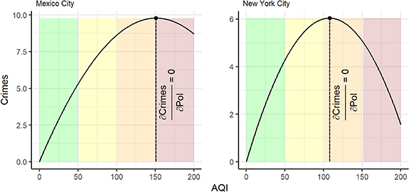
Figure 6. Nonlinear effect of air pollution on criminality.
Download figure:
Standard image High-resolution imageFigure 7 complements the previous exhibit by estimating the marginal effects of exposure on the number of crimes happening around pollution measuring stations in Mexico City and New York. This figure shows the NowCast AQI on the horizontal axis and the first derivative of crime counts concerning exposure on the vertical axis.

Figure 7. Estimated marginal effects of air pollution on crime.
Download figure:
Standard image High-resolution imageComputing the marginal effects allows me to show the negative relationship between the second derivative of criminality concerning the NowCast AQI. As it is clear from the picture, the relationship between both variables reverses at high exposure intervals, suggesting that air pollution significantly increases criminality between 0 and 91 AQIs for New York and between 0 and 139 for Mexico City 19 .
The results from the quadratic design provide parametric evidence of nonlinearities. However, most studies currently looking at the effects of pollution on crime assume a monotonic and increasing relationship between both variables. Fitting linear models into the nonlinear relationship can lead to biased coefficients. For instance, a linear model may show insignificant or negative point estimates in settings with very high average exposure values. This issue is particularly relevant when comparing urban centers, as a stronger positive relationship would arise for cleaner cities (like New York vs. Mexico City).
Although informative regarding the shape of the functional form, the quadratic model does not examine effects across actual concentration intervals, i.e. how large or small criminality is in hours with specific pollution values. Figure 8 solves this by estimating the pollution-crime relationship nonparametrically. The nonparametric design divides air pollution into six self-contained exposure bins between zero and the 99th percentile of the NowCast AQI. The only functional restriction within this methodology is that the effect on criminality is linear within these bins. Nonparametric estimates confirm the nonlinear relationship between pollution and crime. For instance, the effect in Mexico City grows until the 138–172 interval. After this, the effect decreases and is 31.8% smaller (concerning the 138–172 interval) in the last bin. For New York City, the nonlinear effect is even clearer, reaching its maximum between 72 and 90 units and decreasing after that.

Figure 8. Non-parametric estimates of the effect of pollution on criminality.
Download figure:
Standard image High-resolution imageNext, I estimate the linear and quadratic specifications for violent and nonviolent crimes. Violent crimes are homicide, aggravated assault, robbery, and rape, while nonviolent crimes are burglary, larceny, fraud, forgery, and bribery 20 . Table 4 shows the results of this exercise. Point estimates show the risk of assuming a linear model for the relationship between pollution and crime. For instance, linear estimates for Mexico City are insignificant and borderline significant for nonviolent and violent crimes. These estimates are in line with Burkhardt et al (2019) study on the effects of pollution on US crime numbers. However, once I add the correct functional form, coefficients become significant for both crime categories. For New York, although linear estimates are statistically different from zero for both categories, coefficients also increase in size and statistical significance with the quadratic design.
Table 4. Estimates on the effects of air pollution for violent and non-violent crimes.
| Mexico City | New York | |||||
|---|---|---|---|---|---|---|
| Linear model | Quadratic model | Linear model | Quadratic model | |||
| Est. | Linear | Linear | Quadratic | Linear | Linear | Quadratic |
| Violent | ||||||

|

|

|

|

| −0.004 | |
| (0.130) | (0.304) | (0.001) | (0.168) | (0.517) | (0.004) | |
| R.Squared | 0.130 | 0.130 | 0.130 | 0.125 | 0.125 | 0.125 |
| N.Obs | 1433 832 | 1433 832 | 1433 832 | 1510 319 | 1510 319 | 1510 319 |
| BIC | 870 538 | 870 529 | 870 529 | 1085 029 | 1085 040 | 1085 040 |
| Non-violent | ||||||
| 0.197 |

|

|

|

| −0.002 | |
| (0.172) | (0.407) | (0.001) | (0.097) | (0.291) | (0.002) | |
| R.Squared | 0.219 | 0.219 | 0.219 | 0.189 | 0.189 | 0.189 |
| N.Obs | 1433 832 | 1433 832 | 1433 832 | 1510 319 | 1510 319 | 1510 319 |
| BIC | 777 428 | 777 439 | 777 439 | 1597 431 | 1597 444 | 1597 444 |
Notes:
 ,
,  ,
,  . This table shows the effect of the NowCast AQI on the number of crimes occurring in a 2 km radius around pollution measuring stations in Mexico City and New York. Results come from two different PPML panel models. The linear model only controls for the effect of the NowCast AQI, and the quadratic model further includes the squared value of the NowCast AQI as an additional covariate. Interpret point estimates as the percentage change in the number of crimes due to a ten units increase in the NowCast AQI. Violent crimes refer to homicide, aggravated assault, robbery, and rape, while nonviolent crimes refer to burglary, larceny, fraud, forgery, and bribery. The PPML controls for weather covariates alongside year-by-month-by-station, hour, and weekday fixed effects—SEs clustered at the station level.
Significant nonlinear estimates for nonviolent felonies suggest that contrary to previous hypotheses (see Burkhardt et al 2019), it is not only an increase in the taste for violence behind the effect of air pollution on criminality but that air pollution also changes the risk behavior of criminals for nonviolent crimes. As an additional analysis, table 5 shows the outcomes for burglary, homicide, robbery, larceny, sexual offenses, and fraud.
Table 5. Estimates on the effects of air pollution across different crime categories.
| Mexico City | New York | |||||
|---|---|---|---|---|---|---|
| Linear model | Quadratic model | Linear model | Quadratic model | |||
| Est. | Linear | Linear | Quadratic | Linear | Linear | Quadratic |
| Burglary | 0.340 | 0.214 | 0.001 | 0.169 | −0.256 | 0.004 |
| (0.304) | (0.871) | (0.004) | (0.186) | (0.571) | (0.004) | |
| Homicide | 0.521 |

|

| 0.084 | −9.775 | 0.089 |
| (0.850) | (1.824) | (0.007) | (12.396) | (25.925) | (0.132) | |
| Robbery |

|

|

| 0.395 |

| −0.010 |
| (0.137) | (0.346) | (0.002) | (0.281) | (0.887) | (0.007) | |
| Larceny | −0.018 | 0.256 | −0.001 |

|

| −0.002 |
| (0.124) | (0.492) | (0.002) | (0.126) | (0.319) | (0.002) | |
| Sexual crimes | 0.497 |

|

|

|

|

|
| (0.374) | (1.534) | (0.006) | (0.148) | (0.299) | (0.002) | |
| Fraud | 0.336 |

|

| 0.339 | 0.586 | −0.002 |
| (0.243) | (0.917) | (0.003) | (0.318) | (1.173) | (0.009) | |
| Other |

|

|

|

|

|

|
| (0.128) | (0.368) | (0.001) | (0.183) | (0.521) | (0.004) | |
Notes:
 ,
,  ,
,  . This table shows the effect of the AQI on the number of burglaries, homicides, robberies, larcenies, sexual crimes, and frauds occurring in a 2 km radius around pollution measuring stations in Mexico City and New York. Results come from two different PPML panel models. The linear model only controls for the effect of the NowCast AQI, and the quadratic model further includes the squared value of the NowCast AQI as an additional covariate. Interpret point estimates as the percentage change in the number of crimes due to a ten units increase in the AQI. The PPML controls for weather covariates alongside year-by-month-by-station, hour, and weekday fixed effects–standard errors clustered at the station level.
The only significant coefficient in the linear model for Mexico City relates to robbery and other crimes. However, once we include the quadratic value of the NowCast AQI, point estimates are statistically different from zero for homicide, robbery, sexual crimes, fraud, and other crimes. For New York, the table shows significant coefficients in the linear and quadratic models for larceny, sexual offenses, and others, while only significant in the quadratic model for robberies 21 .
6. Robustness
Bondy et al (2020) and Herrnstadt et al (2020) propose that unobservables and measurement error can bias the coefficients of the pollution-crime relationship. They account for this bias by implementing an IV strategy with wind direction as a pollution instrument. Equations (8) and (9) show the empirical specification of an analogous model. In it, NowCastst is the NowCast AQI value of station s at time t and wdrst a matrix of k − 1 dummy variables determining the cardinal direction in which the wind blows for each measuring station 22


Table 6 shows the results from the IV design for the linear and quadratic specifications. Across models, first-stage F-statistics are larger than one hundred, reducing worries regarding the ability of wind direction to predict air pollution. For Mexico City, the IV coefficient grows from 0.20% to an insignificant 0.32%, and for New York, from 0.48% to 1.04%.
Table 6. Effect of air pollution on criminality (IV).
| Linear model | Quadratic model | |||||
|---|---|---|---|---|---|---|
| Mexico City | New York | Mexico City linear estimate | Mexico City quadratic estimate | New York linear estimate | New York linear estimate | |
| 0.327 |

|

|

|

| −0.004 | |
| (0.309) | (0.186) | (0.584) | (0.002) | (0.612) | (0.006) | |
| R.Squared | 0.220 | 0.224 | 0.224 | 0.224 | 0.227 | 0.227 |
| F-stat | 168 | 293 | 150 | 150 | 294 | 294 |
| N.Obs | 1433 832 | 1510 319 | 1433 832 | 1433 832 | 1510 319 | 1510 319 |
| BIC | 1638 450 | 2862 710 | 1635 938 | 1635 938 | 2858 315 | 2858 315 |
Notes:
 ,
,  ,
,  . This table shows the effect of the NowCast AQI on the number of crimes occurring in a 2 km radius around pollution measuring stations in Mexico City and New York. Results come from two different PPML-IV panel models with wind direction as an instrument for the NowCast AQI. The linear model only controls for the effect of the NowCast AQI, and the quadratic model further includes its squared value as an additional covariate. Interpret point estimates as the percentage change in the number of crimes due to a ten units increase in the NowCast AQI. The econometric design additionally accounts for weather controls and year-by-month-by-station, hour, and weekday fixed effects. Bootstrapped standard errors with two-hundred iterations clustered at the station level.
This increase in the size of the coefficient occurs because IVs can only retrieve local average treatment effects. Figure A3 shows box plots for the raw and IV fitted values of the NowCast AQI. As expected, the IV strategy shrinks the value of the NowCast AQI at the extremes of the distribution, with potential relevant effects in the interpretation of point estimates. For instance, Bondy et al (2020) and Herrnstadt et al (2020) also find higher linear estimates when using the IV strategy 23 . Concerning the quadratic model, although quadratic coefficients are only statistically significant for Mexico City, point estimates confirm the inverse U-shaped relationship between pollution and crime. Notably, using the IV strategy can lead to the same issues of insignificant effects in the linear model because of fitting the wrong functional form to the pollution-crime relationship.
Next, table 7 presents the estimates of the preferred specification for the linear and quadratic models across three different estimators; OLS, log-linear OLS, and negative binomial 24 .
Table 7. Effect of air pollution on criminality across different estimators.
| Mexico City | New York | |||||
|---|---|---|---|---|---|---|
| OLS | Log-linear OLS | Negative binomial | OLS | Log-linear OLS | Negative binomial | |
| Linear model | ||||||

|

|

|

|

|

| |
| (0.002) | (0.026) | (0.115) | (0.004) | (0.055) | (0.069) | |
| N.Obs | 1433 832 | 1433 832 | 1433 832 | 1510 319 | 1510 319 | 1510 319 |
| BIC | 2784 659 | 797 576 | 1634 911 | 3869 900 | 1612 538 | 2847 884 |
| Quadratic model | ||||||
| Linear Est. |

|

|

|

|

|

|
| (0.004) | (0.070) | (0.205) | (0.009) | (0.131) | (0.197) | |
| Quadratic Est. |

|

|

|

|

|

|

|

| (0.001) |

| (0.001) | (0.001) | |
| N.Obs | 1433 832 | 1433 832 | 1433 832 | 1510 319 | 1510 319 | 1510 319 |
| BIC | 2784 671 | 797 587 | 1634 895 | 3869 892 | 1612 524 | 2847 882 |
Notes:
 ,
,  ,
,  . This table shows the effect of the NowCast AQI on the number of crimes occurring in a 2 km radius around pollution measuring stations in Mexico City and New York. Results come from two different panel models across three different estimators, OLS, log-linear OLS, and negative binomial. The linear model only controls for the effect of the NowCast AQI, and the quadratic model further includes its squared value as an additional covariate. The econometric design additionally accounts for weather controls and year-by-month-by-station, hour, and weekday fixed effects—standard errors clustered at the station level.
Reassuringly, linear and quadratic results remain statistically significant and in the same direction as the coefficients of the PPML, providing evidence that the functional relationship between pollution and crime does not depend on the econometric estimator.
Table 8 shows the results of four additional robustness exercises. Column (1) contains estimates of a regression model where I assign all crimes within a 2 km radius to each measuring station. The only difference with the standard design is that crimes can now be assigned to more than one station as long as they occur within the 2 km catchment area. In (2), I exclude all observations happening at midday because of the irregular jump in the number of crimes in figure 4. Finally, columns (3) and (4) reduce the catchment radius of measuring stations to 1000 and 500 m.
Table 8. Robustness exercises on the effects of air pollution on criminality.
| Mexico City | New York | |||||||
|---|---|---|---|---|---|---|---|---|
| (1) | (2) | (3) | (4) | (1) | (2) | (3) | (4) | |
| Linear model | ||||||||

|

|

| 0.084 |

|

|

|

| |
| (0.100) | (0.109) | (0.109) | (0.214) | (0.072) | (0.086) | (0.087) | (0.161) | |
| N.Obs | 1374 089 | 1185 552 | 1185 552 | 1116 912 | 1448 121 | 1510 319 | 1510 319 | 1510 319 |
| BIC | 1516 118 | 717 986 | 717 986 | 254 487 | 2728 597 | 2098 240 | 1879 357 | 994 447 |
| Quadratic model | ||||||||
| Linear Est. |

|

|

|

|

|

|

|

|
| (0.226) | (0.290) | (0.290) | (0.647) | (0.196) | (0.327) | (0.323) | (0.602) | |
| Quadratic Est. |

|

|

|

|

|

|

| −0.005 |
| (0.001) | (0.001) | (0.001) | (0.003) | (0.001) | (0.002) | (0.002) | (0.004) | |
| N.Obs | 1374 089 | 1185 552 | 1185 552 | 1116 912 | 1448 121 | 1510 319 | 1510 319 | 1510 319 |
| BIC | 1516 098 | 717 980 | 717 980 | 254 497 | 2728 593 | 2098 239 | 1879 356 | 994 459 |
Notes:
 ,
,  ,
,  . This table shows the effect of the NowCast AQI on the number of crimes occurring in a 2 km radius around pollution measuring stations in Mexico City and New York. Results come from two different panel models across four different robustness exercises. The linear model only controls for the effect of the NowCast AQI, and the quadratic model further includes its squared value as an additional covariate. Column (1) contains estimates of a regression model where I assign all crimes within a 2 km radius to each measuring station. The only difference with the standard design is that crimes can now be assigned to more than one station as long as they occur within the 2 km catchment radius. In (2), I exclude all observations happening at midday because of the irregular jump in the number of crimes occurring at this hour (see figure 4). Finally, columns (3) and (4) reduce the catchment radius of measuring stations to 1000 and 500 m. Interpret coefficients as the percentage increase in criminality due to a ten units increase in the NowCast AQI. The econometric design additionally accounts for weather controls and year-by-month-by-station, hour, and weekday fixed effects—standard errors clustered at the station level.
All point estimates confirm the results of the preferred specification, i.e. positive coefficients in the linear model and positive and negative for the linear and quadratic coefficients in the quadratic model.
Throughout the study, I estimate the impact of exposure on contemporaneous criminality. However, air pollution can either shift crime forward for a couple of hours or, in case there are cumulative effects, increase crime several hours after exposure. To control for crime displacement, I specify a dynamic version of the empirical strategy with a distributed lag quadratic model 25 .
Equation (10) shows the econometric specification of the dynamic model. The only difference to the contemporaneous design is the inclusion of n lagged values of the NowCast AQI in the term  . This specification allows the effect of air pollution up to n days in the past to affect crime today. After estimating a coefficient for each γj
(
. This specification allows the effect of air pollution up to n days in the past to affect crime today. After estimating a coefficient for each γj
(
 ), I aggregate point estimates according to Deschenes and Moretti (2009) study on the relationship between temperature exposure, mortality, and migration in the US (i.e.
  and
and  )
)

Table 9 contains the results of estimating the effects of exposure on criminality with four different values of n. Reassuringly, all linear and quadratic coefficients are in line with the main results, i.e. positive linear and negative quadratic point estimates. Moreover, we can further appreciate the potential negative effect of fitting a linear model to estimate a non-linear relationship, with three out of four distributed lag models implying insignificant coefficients for Mexico City.
Table 9. Effects of air pollution on criminality for different lag models.
| Mexico City | New York | |||||||
|---|---|---|---|---|---|---|---|---|
| Lag 1 | Lag 4 | Lag 8 | Lag 16 | Lag 1 | Lag 4 | Lag 8 | Lag 16 | |
| Linear | ||||||||
| 0.188 |

| 0.114 | 0.099 |

|

|

|

| |
| (0.143) | (0.110) | (0.083) | (0.083) | (0.095) | (0.100) | (0.113) | (0.126) | |
| R.Squared | 0.220 | 0.220 | 0.220 | 0.220 | 0.224 | 0.224 | 0.224 | 0.224 |
| N.Obs |

|

|

|

|

|

|

|

|
| Quadratic model | ||||||||
| Linear Est. |

|

|

|

|

|

|

|

|
| (0.307) | (0.291) | (0.304) | (0.315) | (0.264) | (0.273) | (0.294) | (0.344) | |
| Quadratic Est. |

|

|

|

|

|

|

|

|
| (0.001) | (0.001) | (0.001) | (0.001) | (0.002) | (0.002) | (0.002) | (0.003) | |
| R.Squared | 0.220 | 0.220 | 0.220 | 0.220 | 0.224 | 0.224 | 0.224 | 0.224 |
| N.Obs |

|

|

|

|

|

|

|

|
Notes: ***p<0.01,
 ,
,  . This table shows the effect of the AQI on the number of crimes occurring in a 2 km radius around pollution measuring stations in Mexico City and New York. Point estimates come from distributed lag non-linear model estimates with PPML estimators. We present results for models across four lag structures (1, 4, 8, and 16 h before the crime). All estimates contain weather controls and year-by-month-by-station, hour, and weekday fixed effects. Interpret point estimates as the percentage change in the number of crimes due to a ten units increase in the NowCast AQI—standard errors clustered at the station level.
7. Conclusion
This article proposes that air pollution has a nonlinear (inverse U-shaped) relationship with criminality. On the one side, exacerbated exposure increases the probability of committing a crime by affecting the brain's chemical composition and raising individuals' taste for risk and violent behavior. At the same time, pollution also decreases the matches between criminals and crime opportunities by reducing the number of agents in the market through exacerbated morbidity (e.g. Knittel et al 2016) and avoidance behavior (e.g. Moretti and Neidell 2011).
Causal estimates on the effect of air pollution on criminality come from PPML estimator panel models that exploit the high degree of temporal and spatial variation across and within monitoring stations to estimate the relation between both variables. While linear estimates confirm the findings of previous studies on the positive effect of pollution on criminality (Burkhardt et al 2019, Bondy et al 2020, Herrnstadt et al 2020), quadratic and nonparametric designs further advance our understanding of this relationship by showing that, even though air pollution increases criminality at standard levels, during episodes of exacerbated exposure, the relationship reverses, leading to a concave and nonlinear relationship between both variables.
Future studies on the pollution–crime relationship should take particular care in assessing the correct functional form before automatically assuming a linear effect. Policymakers can use these results in cost-benefit studies of air pollution control policies aiming at the correct implementation of Pigouvian taxes, cap-and-trade mechanisms, or command and control systems. Moreover, we need more information on the neurological pathway through which air pollution affects the no-crime condition and its relationship with criminals or victims' health and avoidance attitudes in the market for criminal activities.
Acknowledgments
I truly appreciate all the constructive comments and suggestions from seminar participants at RFF-CMCC: European Institute on Economics and the Environment. I am very grateful for constructive comments and feedback from Dr Aleksandar Zaklan, Prof. Dr Christian Traxler, Dr Nicole Wägner, and Julia Rechliz. I acknowledge the financial support from the H2020 ERC Starting Grant funded by European Commission (#853487).
Data availability statement
The data that support the findings of this study are openly available at the following URL/DOI: https://www.dropbox.com/sh/9oyfzolf4rz42s6/AABbCWzqnDNQckt60qpniEuMa?dl=0.
: Appendix
Appendix. Data section
Definition of crime categories
- Homicide: the crime of killing a person (it includes manslaughter).
- Aggravated assault: an unlawful attack where the victim suffers severe or aggravated injuries.
- Non-aggravated assault: an unlawful attack where the criminal threatens the victim with the possibility of suffering an aggravated assault.
- Burglary: the crime of illegally entering a building and stealing things.
- Robbery: the crime of taking or attempting to take anything of value by force, threat of force, or by putting the victim in fear.
- Larceny: the crime of taking something that does not belong to you, without illegally entering a building to do so.
- Sex crime: all sex related crimes like rapes, pimping, lewd conduct, or sexual battery with the exception of rape.
- Fraud: includes crimes as theft of identity, document forgery, or defrauding an innkeeper.
- Other: all of the other crimes that are not contained in the previous classifications.
Crimes classification for New York City
- Homicide—homicide and manslaughter.
- Aggravated assault—assault, strangulation, obstruct breathing.
- Non-aggravated assault—menacing, coercion, mischief, tampering.
- Burglary—trespass, possession of burglars' tools, burglary.
- Robbery—robbery.
- Larceny—petite larceny, grand larceny, theft, stolen property, stolen motor vehicle, dog stealing.
- Sex crime—rape, sexual misconduct, sexual abuse, sex crimes, sexual offense, aggravated sexual injury, luring a child, solicitation, facilitation, prostitution, sex trafficking, obscenity, harassment, bigamy, incest, promoting a sexual performance, use of a child in a sexual per, incest, sodomy.
- Fraud—conspiracy, accosting, fortune telling, credit card fraud, theft of services, bribery, bad check, forgery, false records, impersonation, fraud, manufacture unauthorized recording, sale of unauthorized records, enterprise corruption, usury, money laundering, tax law.
- Other—end welfare elderly, reckless endangerment, promoting suicide, abortion, unlawful imprisonment, criminal contempt, arson, posting advertisements, unauthorized use vehicle, jostling, controlled substances, drug paraphernalia, gambling, unlawful possession of a weapon, loitering, disorderly conduct, exposure, healthcare offenses, unlawful assembly, false reports, riot, nuisance, lewdness, terrorism, privacy offenses, eavesdropping, endangering, tampering with a witness, escape, bail jumping, perjury, resist arrest, absconding from work release, computer crimes, weapons possession, fireworks, navigation law, public health law, marriage offenses, environmental control board, traffic offenses, leaving a scene of accident, unlawful parking, health code violation, gratuity, administrative code violation, unlicensed taxi, noise, air pollution, NY state laws, unclassified violation, kidnapping, labor trafficking, custodial interference, unlawful possession of radio devices.
Crimes classification for Mexico City
- Homicide—homicide, femicide, and negligent homicide
- Aggravated assault—aggravated assault and intentional injuries
- Non-aggravated assault—damage to the property of others, intimidation, insults, extortion
- Burglary—home burglary and breaking and entering
- Robbery—violent robbery
- Larceny—robbery without violence
- Sex crime—rape, sexual abuse, sexual harassment, corruption of minors, corruption of disabled, sexual relationships with minor, exhibition of minors, pimping, child pornography
- Fraud—authority abuse, coaching of public servers, illegitimate collection, bribery, concussion, crimes of patron, lawyers, and litigants, electoral crimes, defamation, abusive exercise of functions, improper exercise of public server, concealment, illicit enrichment, false statement, forgery, falsification, fraud, denial of public service, operations with resources of illicit provenance, peculation, break seals, use of false document, misuse of attributions and powers, function usurpation, identity theft, profession usurpation
- Other—abandonment of person, abortion, trust abuse, delicious association, attack on communication ways, assault on public peace, bigamy, land-use-change, pollution or waste, crimes against the civil state, crimes against public officials, crimes against the general law of explosives, guilty of property damage, damage to foreign property, soil damage, human rights violations, environmental crimes, crimes against health, disrespect, disobedience, disposition, discrimination, firearms, prisoner evasion exhort, inhumations or exhumations, food insolvency, negligent injuries, animal abuse, riot, drug dealing, opposition to public work, loss of life due to external factors, prohibited weapons, assisted procreation, provocation of crime, resist arrest, professional liability, reveal secrets, sabotage, illegal wood chopping, suicide attempt, torture, improper use of the public road, correspondence violation, violation of privacy, family violence, forced disappearance, unlawful delivery of a minor, kidnapping, deprivation of personal freedom, theft of infant, express kidnapping, child abduction, infant trafficking, human trafficking.
Appendix. Results section
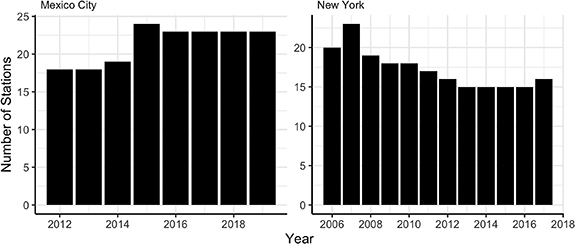
Figure A1. Number of stations per year.
Download figure:
Standard image High-resolution image
Figure A2. Color coded health risks for the EPA air quality index.
Download figure:
Standard image High-resolution image
Figure A3. Box plots of raw and IV-fitted values of the NowCast AQI.
Download figure:
Standard image High-resolution imageTable A1. Effects of air pollution on criminality across different specifications of weather covariates.
| Mexico City | New York | |||||
|---|---|---|---|---|---|---|
| (1) | (2) | (3) | (1) | (2) | (3) | |
| Linear model | ||||||

|

|

|

| −0.003 |

| |
| (0.118) | (0.118) | (0.125) | (0.057) | (0.081) | (0.082) | |
| N.Obs | 1433 832 | 1433 832 | 1433 832 | 1510 319 | 1510 319 | 1510 319 |
| BIC | 1638 127 | 1638 080 | 1638 094 | 3395 871 | 2863 165 | 2862 036 |
| Quadratic model | ||||||
| Linear Est. |

|

|

|

|

|

|
| (0.215) | (0.194) | (0.192) | (0.180) | (0.211) | (0.202) | |
| Quadratic Est. |

|

|

|

|

|

|
| (0.001) | (0.001) | (0.001) | (0.001) | (0.001) | (0.001) | |
| N.Obs | 1433 832 | 1433 832 | 1433 832 | 1510 319 | 1510 319 | 1510 319 |
| BIC | 1638 102 | 1638 048 | 1638 067 | 3395 836 | 2863 164 | 2862 039 |
Notes:
 ,
,  . This table shows the effect of the AQI on the number of crimes occurring in a 2 km radius around pollution measuring stations in Mexico City and New York. I report coefficients for three different specifications of weather covariates. (1) has not weather controls, (2) includes temperature, relative humidity, precipitation, and wind speed linearly, and (3) further adds the square value of temperature and precipitation. Point estimates come PMLE panel models with year-by-month-by-station, hour, and weekday fixed effects. Interpret coefficients as percentage changes in the number of crimes due to a ten units increase in the AQI—standard errors clustered at the station level.
Table A2. Effects of air pollution on criminality across different clustering of standard errors.
| Mexico City | New York | |||||
|---|---|---|---|---|---|---|
| Station plus month | Station plus week | Station plus date | Station plus month | Station plus week | Station plusc date | |
| Linear model | ||||||

|

|

|

|

|

| |
| (0.131) | (0.133) | (0.135) | (0.102) | (0.125) | (0.105) | |
| N.Obs | 1433 832 | 1433 832 | 1433 832 | 1510 319 | 1510 319 | 1510 319 |
| BIC | 1638 127 | 1638 080 | 1638 094 | 3395 871 | 2863 165 | 2862 036 |
| Quadratic model | ||||||
| Linear Est. |

|

|

|

|

|

|
| (0.251) | (0.260) | (0.258) | (0.264) | (0.268) | (0.264) | |
| Quadratic Est. |

|

|

|

|

|

|
| (0.001) | (0.001) | (0.001) | (0.002) | (0.002) | (0.002) | |
| N.Obs | 1433 832 | 1433 832 | 1433 832 | 1510 319 | 1510 319 | 1510 319 |
| BIC | 1638 102 | 1638 048 | 1638 067 | 3395 836 | 2863 164 | 2862 039 |
Notes:
 ,
,  . This table shows the effect of the AQI on the number of crimes occurring in a 2 km radius around pollution measuring stations in Mexico City and New York. Point estimates come from OLS and log-linear OLS panel models with weather controls and year-by-month-by-station, hour, and weekday fixed effects. Interpret coefficients in the OLS model as the marginal effect of increasing each particle by 100 units and in the log-linear design as percentage changes in the number of crimes due to a ten units increase in the AQI—standard errors clustered at the station level.
Footnotes
- 3
- 4
Estimates from wealthier cities can underestimate the health effects of exposure if they are, on average, less polluted and their population healthier.
- 5
In an older version of this study, I also included data for Toronto and Los Angeles. However, data inconsistencies in both cities led me to concentrate on Mexico City and New York.
- 6
See Block and Calderón-Garcidueñas (2009).
- 7
i.e.
![$p [U(y_\mathrm {c}-\beta F)] + (1-p) [U(y_\mathrm {c})] \gt 0$](data:image/png;base64,iVBORw0KGgoAAAANSUhEUgAAAAEAAAABCAQAAAC1HAwCAAAAC0lEQVR42mNkYAAAAAYAAjCB0C8AAAAASUVORK5CYII=) .
. - 8
I justify this theoretical inverse relationship between the number of agents in the market and air pollution with the substantial number of empirical papers finding that air pollution decreases labor supply (Hanna and Oliva 2015, Aragon et al 2017), raise school absences (Currie et al 2009, Chen et al 2018), and increase avoidance attitudes (Zivin and Neidell 2009).
- 9
I complement Mexico City's public data with a citizen request for the years between 2012 and 2015.
- 10
Section 'Data section' contains the definition of each crime category.
- 11
U.S. Environmental Protection Agency (2020).
- 12
Direccion de Monitoreo Armosferico de la Ciudad de Mexico (2020).
- 13
As it is common with studies using station-level data, not all stations operate for the entire sample (see figure A1).
- 14
The size of the sample can change across econometric specifications because some observations are missing weather controls.
- 15
I implement the PPML with the algorithm developed by Correia et al (2020). This algorithm allows me to incorporate high-dimensional fixed effects into the econometric model, adjust for over-dispersion, and obtain high rates of convergence efficiency.
- 16
I also account for the interaction between temperature and relative humidity to consider humans' ability to cool down in humid environments. Additionally, I explore the robustness of point estimates to different specifications of weather covariates in table A1.
- 17
I account for auto-correlated unobservables within measuring stations by clustering standard errors at the station level. However, results are robust to alternative clustering, including two-way clustering at the station-month, station-week, and station-date levels; see table A2.
- 18
Uncovering a positive linear effect of air pollution on crime across four studies with different empirical settings (Burkhardt et al 2019, Bondy et al 2020, Herrnstadt et al 2020) reduces concerns about measurement error, author biases, or spurious correlations behind the qualitative relationship of both variables.
- 19
These threshold values are equivalent to the point where air pollution's effect on criminality is statistically different than zero at the 90% confidence interval.
- 20
There is the possibility of violent burglaries. However, I presume the objective of most burglary cases is to avoid facing the victims. Additionally, both jurisdictions record the most violent crime in cases of multiple felonies. For instance, they record a burglary and homicide case as a homicide instead of a burglary.
- 21
Contrary to Mexico City, the crime data from New York City does not contain homicide counts because it only relies on local-police reports. This lack of homicide data precludes me from accurately estimating the effect of exposure on homicide and manslaughter as there are only 54 cases to determine the impact. Thus, I recommend taking the homicide estimates for New York with a grain of salt.
- 22
Estimating a coefficient for each station and wind direction increases the number of instrumental variables and thus avoids dimensionality issues in the IV design. Moreover, I report cluster-robust bootstrapped standard errors at the station level.
- 23
Even more, point estimates are only significant in Herrnstadt et al (2020) with the IV model, suggesting that perhaps IV's ability to shrink the distribution may exacerbate the positive part of the inverse U-shaped relationship.
- 24
Interpret the OLS estimator as the increase in the number of crimes because of a twenty-five units increase in pollution. The interpretation of coefficients for log-linear OLS and Negative Binomial is analogous to the PPML.
- 25
This model is closely related to the distributed-lag non-linear model commonly used in the epidemiological literature (see Schwartz 2000, Armstrong 2006, Gasparrini 2014) and previously used to estimate the mortality effects of extreme temperatures (e.g. Wang et al 2019, Xing et al 2022), air pollution (e.g. Schwartz 2001, Sun et al 2022), and clinical trials (e.g. Sylvestre and Abrahamowicz 2009).
![$p [U(y_\mathrm {c}-\beta F)] + (1-p) [U(y_\mathrm {c})] \gt 0$](https://content.cld.iop.org/journals/2752-5309/1/2/021001/revision4/erhac9a65ieqn7.gif)