

Abstract
Although the most dire societal impacts of sea-level rise (SLR) typically manifest toward the end of the 21st century, many coastal communities face challenges in the present due to recurrent tidal flooding. Few studies have documented transportation disruptions due to tidal flooding in the recent past. Here, we address this issue by combining home and work locations for approximately 500 million commuters in coastal US counties from 2002 to 2017. We find tidal flooding delays coastal commuters by approximately 22 min per year in 2015–2017, increasing to between 200 and 650 min by 2060 under various SLR scenarios. Adjustments in residential and work locations reduce the growth in commuting delays for approximately 40% of US counties. For residents in coastal counties, SLR is not a distant threat—it is already lapping at their toes.
Export citation and abstract BibTeX RIS

Original content from this work may be used under the terms of the Creative Commons Attribution 4.0 license. Any further distribution of this work must maintain attribution to the author(s) and the title of the work, journal citation and DOI.
1. Main text
Sea-level rise (SLR) is one of the most visible and costly impacts of climate change (Church et al 2013, Oppenheimer et al 2019). With sea levels expected to rise up to 2.5 m by 2100 (Sweet et al 2017, Oppenheimer et al 2019), scientists routinely quantify the potential multitude of impacts of SLR over the next eighty to 2000+ years (Strauss et al 2015, Clark et al 2016, Oppenheimer et al 2019), focusing on impacts deep into the future when they will be presumed greatest.
Although the most worrying societal impacts of SLR (displacement and permanent submergence) typically manifest toward the end of the 21st century (Kulp and Strauss 2019, Oppenheimer et al 2019, Hauer et al 2020), many coastal communities face daunting impacts in the present due to recurrent tidal or high tide flooding (Dahl et al 2017, Moftakhari et al 2017, Sweet et al 2018). We use 'tidal flooding' to refer to only tide-based inundation, i.e. excluding precipitation (Hague and Taylor 2021). Our definition differs from that used by other studies focusing on tidal flooding above minimum thresholds (e.g. Sweet et al 2018) 4 . Studies focusing exclusively on directly affected areas find tidal flooding causes coastal erosion (Hinkel et al 2013), saltwater intrusion (Chang et al 2011), reduced property values (McAlpine and Porter 2018), damaged property (Bukvic and Harrald 2019), submerged transportation routes (Jacobs et al 2018), and exposure of thousands of people to general flood risks (Kulp and Strauss 2019). Given the interconnectedness of coastal communities, e.g. via commuting (Kasmalkar et al 2021), SLR impacts will likely indirectly affect inland, higher elevation coastal areas. The extent to which coastal commutes might be delayed due to inundation on roadways is presently uncertain for the coastal United States.
Some research has linked tidal flooding to transportation networks. These studies use prescribed flood levels rather than historical tide data (Jacobs et al 2018, Kasmalkar et al 2020), limited transportation routes to major roads (Jacobs et al 2018, Kasmalkar et al 2020), annual daily traffic data rather than actual commuter data (Jacobs et al 2018), or limit their analysis to specific areas (Jacobs et al 2018, Kasmalkar et al 2020, Shen and Kim 2020, Hauer et al 2021, Praharaj et al 2021). Most notably, Jacobs et al (2018) and Fant et al (2021) link average annual traffic on major roadways to road inundation and calculate road-segment-specific travel delays in the absence of alternative routing to 'dry' routes. No such national-level estimate of commuting delays presently exist that account for alternative routing to avoid or minimize delays along flooded roadways. These shortcomings combine to create incomplete estimates of SLR and tidal flooding impacts on commuting in coastal communities.
Using national-level routing, commuting, and elevation data, we overcome these issues to estimate the burden SLR driven tidal flooding imposes on commuting times with a dynamic routing algorithm to allow for commuters to route around flooding-related delays. By combining commuter data with detailed road networks in a flood hazard model we assess the commuting delays associated with present and future SLR driven tidal flooding.
Our analytical framework addresses three primary questions concerning SLR impacts in coastal communities in the United States: (1) What is the current commuting time burden imposed by SLR driven tidal flooding and what areas does SLR driven tidal flooding burden the most? (2) How have changes in commuting behavior and residential location affected this burden? And (3) What is the future commuting time burden, absent further behavioral changes?
We estimate commuting delays attributable to recurrent tidal flooding by combining multiple large-scale georeferenced data sources within a travel optimization routine. Namely, we combine (1) the home and work (HW) locations for 74 million census block group (CBG) located in 222 coastal counties and 158 non-coastal counties for 500 million commuter-years in the period 2002–2017 (U.S. Census Bureau 2020), (2) a complete road network from Open Street Map (OpenStreetMap contributors 2017), (3) data from eighty-four tide stations across the US from National Oceanographic and Atmospheric Administration's (NOAA) Center for Operational Oceanographic Products and Services (CO-OPs) tide gauge database (Chamberlain 2020, NOAA CO-OPs 2020), (4) the National Levee Database (US Army Corps of Engineers 2020), and (5) digital elevation models from both NOAA (NOAA 2020) and the US Geological Survey (Gesch et al 2002).
We converted OSM's street network into dual-weighted directed graphs and calculated the minimum travel times between HW CBGs, conditional on flood depth on roadways, between 2002 and 2017 and projected in 2060 using NOAA's global mean SLR scenarios (Sweet et al 2017). As roadways become inundated over time and travel velocity slows, we dynamically adjust travel routes to ensure commuters select the path with the least travel time for a given amount of roadway inundation. Both the change in the commuters along a HW pair and the change in tide heights due to SLR contribute to changes in commuting delays over time. Changes in commuters along a HW pair can theoretically reflect adaptive residential or work location changes to reduce flood-related commuting delays—all else equal—and we isolate this behavior using a two-factor decomposition (Gupta 1991). We refer to this adaptive behavior as 'accommodation', as opposed to 'retreat' or 'adaptation' broadly, since it is an adaptation response that reduces vulnerability to commuting delays without protection or necessarily retreat (Oppenheimer et al 2019).
2. Methods and materials
First, we describe the data sets used in our analysis. Second, we describe the methods to estimate commuting delays.
Data. We use five primary data sources to estimate commuting delays: commuting information, road network data, tide gauge data, levee data, and digital elevation models.
Commuting information comes from the U.S. Census Bureau's Longitudinal Employer-Household Dynamics (LEHD) Origin-Destination Employment Statistics (LODES) for the period 2002–2017 (U.S. Census Bureau 2020). LEHD-LODES is a partially synthetic dataset for paired CBG residential (home) and employment (work) locations in the United States. We downloaded these data for all coastal counties (n = 222), limiting our analysis to respondents with differing home and work CBGs. For computational tractability, we subset the complete 'commuting area' of any given coastal county to those counties that are (i) within 100 miles of the coastal county centroid, and that (ii) contain at least 1% of the commuters into the coastal county. As illustrated in figure 1, on average this procedure captures nearly 90% of a county's commuters (median 89%, 80% of counties capture at least 81% of commuters). Overall, it yields 74 million CBG origin-destination pairs.

Figure 1. Distribution of county commuters within 100 miles of destination county and containing at least 1% of commuters. The median county captures approximately 90% of commuters.
Download figure:
Standard image High-resolution imageDue to unavailability of historical data, data sharing limitations, or quality assurance problems, three states in our analysis have incomplete commuting data: New Hampshire in 2002, Mississippi in 2002 and 2003, and Massachusetts from 2002–2010. Massachusetts lack of data for 2002–2010 also impacts New Hampshire, as nearly 30% of New Hampshire commuters are missing between 2003 and 2010. All other states contain complete commuting data for the entire period. We therefore exclude Mississippi commuters prior to 2004 and Massachusetts and New Hampshire commuters prior to 2011.
We obtain road network data from Open Street Map (OSM). OSM is an open-source, free, editable map of world street networks and features built from volunteers. OSM data include speed limits, network connectivity, and road segment characteristics useful for our analysis such as 'tunnel' and 'bridge.' Previous analyses of the completeness and accuracy of OSM data suggest sufficient georeferenced accuracy (El-Ashmawy 2016, Brovelli et al 2017). We obtain all road network types (primary, motorway, residential, etc) except for service road types for any destination coastal county, any origin commuter county within 100 miles and containing at least 1% of commuters, and any county in between for our analysis.
We obtain tide gauge data for 84 tide stations across the US from NOAA's Center for Operational Oceanographic Products and Services (CO-OPs) tide gauge database. Figure 2 shows the geographic distribution of tide gauages. We download hourly verified water heights for the period 2002–2019 using the 'rnoaa' package (Chamberlain 2020), in the R programming language and subset the tide gauges for the max water height during readings between the hours of 05:00 and 20:00 for Monday through Friday—the primary commuting days and hours in most areas. We normalize the annual number of commuting days to a standardized 250-day year. To correct for extreme water levels which might correspond with extreme weather events such as tropical cyclones, we use an outlier detection algorithm (Chen and Liu 1993, de Lacalle 2019) to search and correct for these extreme water levels by building counterfactual tide gauge series. We use the counterfactual value in time periods where the observed gauge reading exceeds  (t-score), correcting only the most extreme water levels. We assign a tide gauge to each county based on shortest distance as the crow flies. For computational tractability, we group tide gauge readings into five discrete bins corresponding to the <90th, <98th, <99.5th, <99.9th, and >99.9th percentiles for each gauge.
Figure 2. Geographic distribution of the 84 tide gauges used.
Download figure:
Standard image High-resolution imageNotably, the two periods in our historical analysis (2002–2004 and 2015–2017) take place at different points in both the perigean and El Niño cycles (Goodman et al 2018). Consequently, this analysis is best interpreted as measuring the effects of changes in water levels between these periods resulting from the combined impact of all influences of water levels at tide gauges, rather than those attributable to global warming-induced sea level rise alone.
Levee data come from the National Levee Database (NLD) maintained by the US Army Corps of Engineers. The NLD is a nationally comprehensive database on levee systems in the United States. We obtained georeferenced levee information for the 22 states in our analysis.
Digital elevation models (DEMs) come from two sources. For areas threatened by SLR we use NOAA's Digital Coast, which is based on 1/9 arcsecond (10 m) or less horizontal resolution. For counties outside of NOAA's coverage, we download DEMs from the National Elevation Dataset (NED) at 1/3 arcsecond resolution (Gesch et al 2002).
Methods. We calculate commuting delay in five steps (Hauer et al 2021). First, we model road inundation depth as a function of a given tide gauge reading. Second, we model travel velocity for each road segment as a function of inundation. Third, we select the fastest route between any two points, conditional on this velocity. Fourth, we use the observed distribution of annual tide gauge readings to calculate the average annual flooding delay for a given pair of points. Fifth, we obtain aggregate commuting delays for any given area as the weighted average annual delay over all home-work location pairs, with weights corresponding to the number of commuters traveling from a given home location to a work location in the period.
Step 1: Road inundation as a function of tide guage.
We combine road network, DEM, levee, and tide gauge data to calculate flood inundation for each road segment. We apply a 'bathtub' hydrological model, similar to NOAA's tidal flooding mapping procedure 5 , calculating road segment inundation levels as the difference between the water levels reported at the tide gauge and the road surface elevation. Any road segment in the OSM wholly located inside of the area of a levee is given an elevation of 100 m, setting its elevation far above any flood height, and any road segment partially located inside of the area of a levee (e.g. when a road segment begins outside of a levee and terminates inside of a levee) we assume the road segment elevation is the mean of the two points. Any road segment located outside of any DEM for any reason (due to being either very far inland via a circuitous route) is also assigned an elevation of 100 m.
To aid in computational tractability, we divide tide gauge data into the five discrete bins outlined above. With each road segment assigned an elevation value, z, we subtract tide gauge bin gb from road segment z to produce the flood depth i for any given segment.
Step 2: Travel velocity as a function of local inundation.
We model travel velocity v in mph along any given road segment as a function of the speed limit L and the mm of road inundation i:
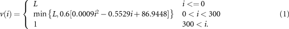
This is the depth-disruption function fitted by Pregnolato et al (2017) but modified in four key ways. First, if a road segment elevation z is above the tide gauge level gb and thus road inundation i is less than 0, we assume vehicle speed is the speed limit, i.e. the road segment is unaffected by tidal flooding. Second, if flooding is less than 300 mm, we assume vehicle speed to be the minimum of the speed limit or the maximum safe speed estimated by Pregnolato et al (2017). This ensures when the maximum safe speed is above the speed limit, we assign travel velocity as the speed limit. Third, we assume a maximum safe speed of one mph, rather than zero, after inundation reaches 300 mm, which is the average depth at which passenger vehicles start to float. Fourth, any road segment in the OSM listed as either a 'tunnel' or a 'bridge' is presumed to be unaffected by road inundation and thus is assigned the speed limit.
Step 3: Calculating optimal travel times.
To find the optimal travel route between two points we first identify each individual origin (home) and destination (work) location conditional on tide gauge bin gb . We assume that the precise location of each origin and destination is the population weighted mean center for each CBG. We then locate the nearest road segment to each population weighted mean centroid as the origin and destination.
Road networks can be conceptualized as dual-weighted directed graphs where the weight is given as the travel velocity. We use the dodgr (Padgham 2019) package in R to convert each county's road network into a dual-weighted directed graph. The travel time along each road segment is calculated based on the segment's length and its speed limit, producing a 'weighted' travel time along a road segment. The travel time between any two points is then calculated as the sum of the weight values. The 'fastest' route is simply calculated as the minimal total sum of weight values for all routes between two points. We calculate the fastest route between each origin and destination CBG under each tide gauge bin b and one 'dry' route, assuming the absence of any flooding.
Step 4: Average annual flooding delays for each home-work pair.
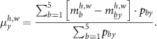
Let  denote daily mean annual flooding delay in min per commuter for any HW pair (h, w) in year y. It is the weighted average difference between the commute time conditional on the inundation level implied by tide bin b,
  , and the 'dry' commute time
  , with weights pby
, the number of days in year y with tide levels in bin b:
, with weights pby
, the number of days in year y with tide levels in bin b:
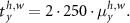
Since the number of workdays varies year to year, we calculate the total annual round trip tide-induced delay per commuter for a normalized 250 workday year as
Given a number of commuters,  , the total min of delay for (h, w) is then
Step 5: Projected SLR commuting delays.
To compute anticipated water depths in 2060, we add the change in NOAA global mean low, intermediate, and extreme SLR scenarios in Sweet et al (2017) to the underlying tide distributions for each tide gauge. These scenarios correspond with 2100 SLR values of 0.3 m, 0.9 m, and 2.5 m, respectively, which translate to 2060 values of 0.19 m, 0.45 m, and 0.9 m. Our projections assume no changes in the shape of the distribution of annual tide values, just a shift in the distribution (Kirezci et al 2020, Taherkhani et al 2020).
Accommodation effects from tide effects.
For any given (h, w) pair between 2002 and 2017, changes in total commuting delays can come from two main changes: a change in the number of commuters (which we refer to as the 'accommodation effect') and a change in the tide values (which we refer to as the 'tide effect'). We employ a Das Gupta decomposition (Gupta 1991) to isolate the change in commuting delays attributable to these two factors. For a given (h, w) pair and two periods (1,2) the change in the total delay can be expressed:
3. Results
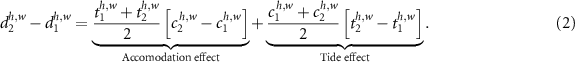
Our models show that tidal flooding delayed the average commuter by a total of 23.3 min in 2017 (figure 3). The total delay increased from 11.9 in 2002—more than doubling in fifteen years. Even with some of the lowest SLR scenarios (0.3 m by 2100), this commuting delay is projected to increase by a factor of seven by 2060 (183 min) and could increase by a factor of twenty-four under high end SLR scenarios by 2060 (643 min with 2.5 m of SLR by 2100).
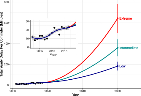
Figure 3. Commuting delays in the United States, 2002–2017 and in 2060 under varying SLR scenarios. Estimates reflect total annual commuting delay for workers employed in coastal communities. Colored dots in 2060 correspond to predicted tide levels based on NOAA SLR curves (Sweet et al 2017) for low (0.3 m), intermediate (1.0 m), and extreme (2.5 m) by 2100. Uncertainty reflects the 90th percentile confidence or prediction interval. Sea-level rise is already delaying US coastal commuters.
Download figure:
Standard image High-resolution imageAll coastal US states experience tidal-flood induced commuting delays and an increase in these delays since 2002 (figure 4). In 2015–2017, Georgia (251 min), North Carolina (92.4 min), and Massachusetts (64.5 min) were the only states with more than one hour of annual commuting delays (table 1). By 2060, even low-end SLR (0.3 m by 2100) will increase commuting delays in coastal areas by an order of magnitude within the next forty years without some form of adaptation.

Figure 4. Commuting delays in US States, 2002–2017. Estimates reflect total annual commuting delay for workers employed in coastal communities. Results for Mississippi in 2002/2003, and New Hampshire and Massachusetts in 2002–2010 excluded due to data quality issues. Every coastal state experiences some amount of SLR commuting delay and all states experience increased delays since 2002.
Download figure:
Standard image High-resolution imageTable 1. Average Annual Commuting Delays in min for US States, 2002–2060. 2060 Intermediate (low‐extreme) values refer to SLR under three 2100 scenarios — 1.0 m [0.3 m - 2.5 m]. These correspond to SLR in 2060 of 0.45 m [0.19 m - 0.9 m].
| State | 2002–2004 | 2015–2017 | % Increase | 2060 Intermediate [low‐extreme] | state | 2002–2004 | 2015–2017 | % Increase | 2060 Intermediate [low‐extreme] |
|---|---|---|---|---|---|---|---|---|---|
| TOT | 9.94 | 22.4 | 126% | 359 [183 - 643] | MS | — | 0.0711 | — | 16.5 [2.42 - 31.9] |
| AL | 7.59 | 16.5 | 117% | 326 [136 - 495] | NH | — | 13.4 | — | 227 [118 - 513] |
| CA | 19.6 | 32.2 | 66% | 457 [246 - 725] | NJ | 9.45 | 20.9 | 123% | 411 [193 - 782] |
| CT | 0.469 | 0.797 | 69% | 27.6 [9.58 - 62.9] | NY | 11.4 | 18.4 | 60% | 325 [174 - 652] |
| DE | 2.59 | 3.94 | 51% | 223 [58.2 - 545] | NC | 55.8 | 92.4 | 66% | 2052 [864 - 3669] |
| FL | 1.64 | 7.54 | 360% | 109 [53.4 - 159] | OR | 13.1 | 19 | 45% | 209 [119 - 385] |
| GA | 86.1 | 251 | 192% | 2794 [1451 - 5296] | RI | 0.108 | 0.178 | 63% | 5.3 [2.14 - 9.55] |
| LA | 6.11 | 7.98 | 30% | 687 [155 - 1189] | SC | 10.6 | 34.2 | 225% | 362 [194 - 586] |
| ME | 4.05 | 7.54 | 87% | 91.3 [51.1 - 187] | TX | 0.0753 | 0.148 | 96% | 3.7 [1.19 - 7.38] |
| MD | 2.3 | 5.46 | 138% | 186 [68.8 - 284] | VA | 5.97 | 14.9 | 150% | 269 [130 - 476] |
| MA | — | 64.5 | — | 1051 [560 - 2148] | WA | 4.73 | 8.3 | 75% | 92.6 [53.4 - 168] |
Commuting delays are unevenly distributed across space (figure 5). For many coastal counties, SLR commuting delays are presently minimal with the median annual commuting delay of just over 3 min in 2017 but by 2060 with intermediate SLR, we estimate the median annual commuting delay will increase to 99.5 min. Three counties—Washington NC (3057 min), McIntosh GA (1275 min), and Tyrrell NC (695 min)—experience over 500 min of annual delay. Twenty-three counties experienced more than 100 min of commuter delay in 2017—approximately the median delay in 2060 under intermediate SLR. For the residents in these counties, SLR is not a distant threat—it is already lapping at their toes.
Figure 5. Annual Commuting delays in 2015–2017 and in 2060 with intermediate SLR (0.9 m by 2100) for US counties. Counties not included in the study area are colored in gray.
Download figure:
Standard image High-resolution imageUnlike population exposure to inundation (Hauer et al 2016), which heavily threatens the US South, SLR impacts are not isolated to specific regions of the US. Places like San Francisco CA, Boston MA, and Savannah GA already see significant commuting delays due to recurrent tidal flooding. These are areas with high king tides, generally longer distance commutes, roadways along low-elevation coastlines, and generally, few, if any, alternative routes. Other major population centers, like Houston TX, Los Angeles CA, and New York NY, presently experience minimal, if any, commuting delays attributable to more alternative routes along higher-elevation inland areas. Areas with the greatest delays tend to contain more long-distance commutes, along roadways with higher maximum speed, containing fewer alternative, 'drier' routes.
Additionally, we investigate how adjustments to commuter home or work locations (or both) have affected commuting delays. Some HW pairs might experience increasing delays due to tidal flooding but decreasing delays due to changes in the number of commuters along that HW pair. These changes are unlikely to be due to technological shifts to increased remote work as the number of non-commuters (i.e. those commuting to the CBG in which they reside) accounted for 1.33% of commuters in 2002 and 1.39% in 2017, suggesting little increase in 'home commuting.'
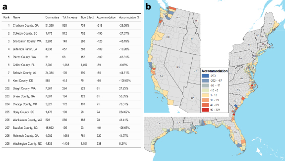
We decompose the change between 2002–2004 and 2015–2017 into the contributions from rising water levels and to changes in the allocation of commuters along HW pairs (what we call the 'accommodation effect'(Hauer et al 2021)) using a two-factor Das Gupta style decomposition (Gupta 1991) for HW pairs with non-zero commuting delays in 2015–2017 (see Methods). Changes in commuter behavior regarding choices of residential and workplace location reduced the impact of flooding delays in 95 (43%) counties (figure 6). However, these accommodation effects are not uniform across the US coast. In parts of California, Georgia, and Florida, for example, the number of commuters increased in highly affected routes, further exacerbating flood-induced delays.
Figure 6. Accommodation to commuting delays between 2002–2017 for Home-Work pairs with non-zero impacts in 2015-2017 for US counties . (a) shows the top and bottom eight counties with the greatest and least Accommodation effects. 'Commuters' refers to the number of commuters with non-zero commuting delays in 2015–2017. 'Tot Increase' refers to the total increase in commuting delays between 2002 and 2017. 'Tide Effect' is the raw increase in commuting delays if the home-work commuters remained unchanged in 2002–2004 but exposed to tides in 2015–2017. 'Accommodation' refers to the decomposed effect due to changes in either home or work locations between 2002–2004 and 2015–2017 with tides kept constant in 2002–2004. (b) maps these accommodation effects. Counties not included in the study area or excluded due to data limitations are colored in gray.
Download figure:
Standard image High-resolution image
4. Discussion
Understanding of SLR thresholds at which people adopt adaptive behavior to reduce their exposure and vulnerability to SLR impacts remains severely limited (Hauer et al 2020), though there is a general understanding that people theoretically must adapt to or accommodate higher water levels. Most examples of contemporary SLR adaptation tend to focus on large governmental infrastructure projects such as deployment of pumps or protective infrastructure (Fu et al 2017), whereas examples of individual adaptation strategies are mostly limited to either theoretical options for coastal residents (Kwadijk et al 2010) or localized case studies with minimal identification of thresholds or tipping points (Jamero et al 2017). Here, we describe how changes in commuter behavior across the coastal US have amplified or reduced the impact of rising tides on commute times. It remains to be seen whether some of the anticipated commuting delays (figure 5 and supplementary material) over the coming decades leave enough space for further accommodation to occur without large scale intervention.
Much of the literature surrounding SLR impacts assesses flood impacts on housing (Hallegatte et al 2013, Hinkel et al 2014), critical infrastructure (Heberger et al 2011, Storlazzi et al 2018), or populations (Strauss et al 2015, Kulp and Strauss 2019). Temporal horizons associated with these impact assessments can be as short as 100 years (Hinkel et al 2014) and as long as 2000 years (Strauss et al 2015), pushing much of these impacts into the deep future. Additionally in many of these impact assessments, what is 'impacted' is defined by residence within a flooded area. Our results demonstrate two important considerations for SLR impact assessments. First, SLR impacts in the form of commuting delays are presently occurring in US coastal communities. In principle, changes in commuter behavior could ameliorate these delays if people were to choose HW locations less vulnerable to tidal flooding. Although we are not able to determine a causal relationship between flood exposure and commuting choices, it does not appear that such accommodating behavior adaptations have been sufficiently widespread as to effectively counter the effect of rising tides. Changes in commuter behavior between 2002 and 2017 reduce flooding delays in less than half of the counties compared to a counterfactual in which residential and workplace locations did not change. Assuming a value of time equal to the median hourly wages of workers in 2019 in each county 6 , the cost of commuting delays increased from $154.7 M in 2002 to more than $439.7 M in 2017. Without significant additional accommodation, adaptation, or mitigation of carbon emissions, these costs could top $3.4 B in 2060 with low SLR or $11.8 B with extreme SLR. These estimates of lost wages are considerably lower than Fant et al (2021)'s estimates of economic damages of $1.3–$1.5 B in 2020 and $28–$37 B in 2050 likely due to our inclusion of alternative routing along 'drier' routes. Second, impacts are not limited to residents immediately adjacent to a coastline but extend to commuters elsewhere (see supplementary figure 1 for an interactive map). Repeated obstruction of transportation routes can impede the flow of goods, affecting business operating costs, employment opportunities, and the cost of living in the long term. Limiting research to flooding impacts of storm surges or inundation on property values underestimates potential SLR impacts in flooding-adjacent areas.
Calls to uncover more specific SLR impacts beyond just flood risk (Hauer et al 2020) make clear the importance analyzing SLR impacts as integrated natural and social systems. For example, recent findings concerning reduced property values in repetitive flood loss areas (McAlpine and Porter 2018), soil salinization on agricultural livelihoods (Chen and Mueller 2018), and climate gentrification responses to SLR flooding (Keenan et al 2018) are some such mechanisms integrating natural and social systems together. In this article, we investigate another specific mechanism in the form of recurrent tidal flooding on commuting delays. In the future, scientists should consider more integrated natural-social systems when investigating SLR impacts, moving beyond just flood hazard and flood risk into the actual social systems in coastal communities.
We make several simplifying assumptions for computational tractability. We assess road water depth with a bathtub model that assumes perfect hydrologic connectivity, potentially overestimating the inundation on roadways. Tidal flooding adversely impacts local drainage systems and since we do not model precipitation, we do not include the possibility of roadway inundation due to rainfall and tidal flooding, potentially underestimating the inundation on roadways (Gold et al 2023). Our model does not account for traffic congestion or public transportation, nor does it include the less than 1.5% of people who live and work within the same CBG, potentially underestimating the commuting delays. Finally, most tidal flooding occurs for several hours, possibly coinciding with morning, evening, or both commutes, depending on when and for how long the high tide lasts. By simplifying to round trip, it is possible we overstate our results.
Data availability statement
The data that support the findings of this study are openly available in the Harvard Dataverse at https://doi.org/10.7910/DVN/2UT4GM (Hauer 2023).
Footnotes
- 4
- 5
- 6
US Census Bureau's American Community Survey tableID: S2001 median hourly wages of workers over age 16 with earnings in 2019.
Supplementary data (85. MB HTML)
Supplementary data (0.1 MB PDF)