

Abstract
In response to a positive CO2 forcing, the seasonal Arctic warming pattern is characterized by an early winter maximum and a summer minimum. While robust, our fundamental understanding of the seasonal expression of Arctic surface warming remains incomplete. Our analysis explores the relationship between the seasonal cycle of surface heating rate changes and the seasonal structure of Arctic warming in modern climate models. Consistent across all models, we find that the background summer-to-winter surface cooling rate and winter-to-summer surface heating rate slows over sea ice regions in response to increased CO2. The slowing of the background summer-to-winter surface cooling rate leads to an early winter Arctic warming maximum, whereby regions and models with a greater slowing also produce a greater winter warming peak. By decomposing the contributions to the background seasonal heating rate change, we find that reductions in sea ice cover and thickness are primarily responsible for the changes. The winter warming peak results from the loss of sea ice cover, which transitions the Arctic surface from a lower thermal inertia surface (sea ice) to a higher thermal inertia surface (ice-free ocean) that slows the seasonal cooling rate. The seasonal cooling rate in autumn is further slowed by the thinning of sea ice, which allows for a greater conductance of heat from the ocean through the sea ice to the surface. These results offer an alternate perspective of the seasonality of Arctic warming, whereby the changing thermal inertia of the Arctic surface is an important aspect of the seasonality, complementary to other perspectives.
Export citation and abstract BibTeX RIS

Original content from this work may be used under the terms of the Creative Commons Attribution 4.0 license. Any further distribution of this work must maintain attribution to the author(s) and the title of the work, journal citation and DOI.
1. Introduction
In response to the anthropogenic increase of greenhouse gases, observations and climate projections indicate that the Arctic surface warms more rapidly than any other region on Earth (Manabe and Wetherald 1975, Ramanathan et al 1979, Holland and Bitz 2003, Cai 2006, Serreze et al 2009, Screen and Simmonds 2010, Pithan and Mauritsen 2014), termed Arctic amplification (AA). However, Arctic warming does not manifest evenly throughout the year; it exhibits a pronounced seasonality—minimum in summer and maximum in early winter (Holland and Bitz 2003, Lu and Cai 2009, Sejas et al 2014, Laîné et al 2016, Boeke and Taylor 2018). Accurate projections of this seasonal structure are important because this feature of Arctic climate change dictates seasonally dependent impacts on climate dynamics and on human and ecological systems (Post et al 2009, Xu et al 2013, Ernakovich et al 2014). Additionally, the largest uncertainty in Arctic warming projections coincides with the maximum warming in early winter (Pithan and Mauritsen 2014, Laîné et al 2016, Boeke and Taylor 2018, Hu et al 2022). Assessing the causes of this uncertainty and constraining the inter-model spread in Arctic warming requires a better understanding of the physical mechanisms and processes responsible for the seasonal warming pattern (Taylor et al 2022).
Varying explanations for Arctic warming and its seasonal pattern have been proposed. Longwave (LW) feedbacks, associated with increases in downwelling LW radiation at the surface, have been proposed as a leading contributor to the seasonal expression of AA (Winton 2006, Lu and Cai 2009, Bintanja and van der Linden 2013). Cloud feedbacks enhance downward LW radiation to the surface through increases in polar clouds during polar night (Holland and Bitz 2003, Vavrus 2004, Sejas et al 2014). Temperature feedbacks, associated with atmospheric warming, also amplify Arctic warming by enhancing the downward LW radiation to the surface (Pithan and Mauritsen 2014, Sejas and Cai 2016). For example, studies find that increased poleward heat transport amplifies Arctic warming by warming the polar atmosphere, which enhance the downward LW radiation to the surface (Alexeev et al 2005, Cai 2006, Cai and Lu 2007, Lu and Cai 2010, Cai and Tung 2012). Stuecker et al (2018) points to the lapse-rate feedback as the main contributor to AA and its seasonal pattern. A few studies also suggest that the weaker Planck feedback (a smaller increase in LW emissions per unit of warming) at colder temperatures also contributes to AA and its seasonal warming pattern (Ohmura 1984, Pithan and Mauritsen 2014, Laîné et al 2016, Sejas and Cai 2016).
An accumulating number of studies indicate that sea ice loss is fundamental to the magnitude of Arctic warming and its seasonal pattern (Manabe and Stouffer 1980, Robock 1983, Mann and Park 1996, Holland and Bitz 2003, Hall 2004, Serreze et al 2009, Screen and Simmonds 2010, Serreze and Barry 2011, Dwyer et al 2012, Bintanja and van der Linden 2013, Kim et al 2016, 2019, Boeke and Taylor 2018, Dai et al 2019, Boeke et al 2021, Hu et al 2022, Liang et al 2022). Some studies indicate that the increase in shortwave (SW) absorption due to the reduction of the surface albedo (i.e. the surface albedo feedback (SAF)) associated with the loss of sea ice is the largest contributor to Arctic warming (Hall 2004, Taylor et al 2013, Yoshimori et al 2014). Locking the surface albedo, Hall (2004) shows SAF increases Arctic warming by 60%–100% and AA by ∼33%. A similar locking study by Graversen and Wang (2009) on a more sophisticated model, however, indicates SAF 'only' increases Arctic warming by ∼30% and AA by ∼15%. Moreover, the seasonal structure of the SAF (maximum in summer when Arctic warming and AA are minimum) suggests that there are other sea ice loss processes responsible for the seasonal Arctic warming pattern.
The impact of sea ice loss on the seasonality of Arctic warming manifests through the summer-to-winter transfer of energy and the change in surface thermal inertia (Hu et al 2022, Taylor et al 2022). Despite the increase in SW absorption, summer warming is muted due to the higher heat capacity of the newly exposed ocean mixed layer and the melting of sea ice. The additional heat is stored by the ocean mixed layer and delays the formation of sea ice or reduces its thickness (Manabe and Stouffer 1980). Inter-model variations in the increase of ocean heat storage, seasonal transfer, and release are shown to correlate well with the inter-model Arctic warming spread (Boeke and Taylor 2018). A few studies also indicate that the delay in sea ice formation during fall/winter increases the thermal inertia of the Arctic surface (i.e. greater effective heat capacity), which slows the seasonal cooling of the Arctic surface during fall and winter contributing to the pronounced winter warming response (Robock 1983, Dwyer et al 2012, Hahn et al 2022).
Most studies point to the reduction of the thermal insulation effect of sea ice in fall and winter, known as the ice-insulation feedback, as the leading cause of the seasonal Arctic warming pattern. The ice-insulation feedback results in a large increase in upward energy release via surface turbulent heat fluxes and upward LW radiation due to the removal of sea ice (Manabe and Stouffer 1980, Screen and Simmonds 2010, Burt et al 2015, Dai et al 2019). The increase in surface-to-atmosphere energy fluxes warms and moistens the lower troposphere and increases fall/winter cloud cover (Kay and Gettelman 2009, Taylor et al 2015, Morrison et al 2019). As a result, downward LW radiation to the surface is enhanced, amplifying the fall/winter warming maximum (Kim et al 2016, 2019). From this description, it is clear that sea ice and LW feedbacks are interconnected.
While a conglomeration of studies point to the importance of sea ice loss on the seasonality of Arctic warming, the relative importance of different sea ice mechanisms is still unclear. Is the ice insulation effect or sea ice cover loss primarily responsible for the seasonality of Arctic warming? Similarly, are changes in heat capacity or surface energy fluxes due to sea ice loss more important to the seasonal warming pattern? Do the processes responsible for the seasonality of Arctic warming also contribute to the large intermodel Arctic warming spread? In this study we use model simulations from the 5th phase of the Coupled Model Intercomparision Project (CMIP5) to investigate the impact of sea-ice loss on the seasonal pattern and magnitude of Arctic warming. To determine the influence of sea-ice loss relative to other surface types, we stratify the seasonal Arctic warming by surface type (land, ocean, and sea-ice regions). We also evaluate the relationship between changes in the seasonal heating rate and the magnitude and seasonality of Arctic warming. This is followed by an analysis of the relationship between sea-ice loss and the inter-model Arctic warming spread. The paper concludes with a discussion and summary.
2. Data and methodology
In this study, we analyze data from atmosphere-ocean general circulation models (table S1) that participated in the 5th phase of the Coupled Model Intercomparison Project (CMIP5). Specifically, two types of CMIP5 experiments (Taylor et al 2012) are used: (1) historical simulations (1850–2005) with time-varying forcing consistent with observations, and (2) representative concentration pathway 8.5 (RCP8.5) climate simulations (2006–2100) that simulate a future climate with radiative forcing reaching ∼8.5 W m−2 by year 2100. CMIP5 data are derived from the monthly mean outputs of the Historical and RCP8.5 model simulations (see Data availability statement). For each model, monthly-mean surface skin and air temperatures, surface downwelling and upwelling shortwave fluxes, surface downwelling and upwelling LW fluxes, and surface upward sensible and latent heat fluxes on its native atmospheric grid are obtained. Sea ice concentration, sea ice surface temperature, snow depth on top of sea ice, and sea surface temperature on their native ocean grids are also obtained. Monthly-mean climatological values of these variables are calculated by averaging 30 years in the historical simulations (1976–2005) and RCP8.5 simulations (2071–2100). Climatological changes of these variables are determined by subtracting the historical values from the RCP8.5 values. For the climatological seasonal heating rate calculation, the month-to-month temperature changes (i.e. Jan-Dec, Feb-Jan, Mar-Feb, etc) are calculated prior to taking the climatological average.
Arctic grid points (60 N–90 N) are divided into land, ocean, and sea ice surface types using the historical climatology. Sea ice grid points are defined as those with a sea ice concentration greater than zero in the historical climate, while ocean grid points are sea ice free. For each model, atmospheric grid variables are interpolated to the corresponding ocean grid.
3. Results
3.1. Surface type dependence of Arctic warming seasonality
Stratifying the Arctic by surface type (sea ice, ocean, and land), we find differences in the magnitude and seasonality of the surface temperature ( ) and its change
  under CO2 forcing between surface types (figure 1). In the historical (late 20th century climate) and RCP8.5 (late 21st century climate) simulations (figures 1(a)–(c)),
  shows a pronounced annual cycle for sea ice and land surfaces compared to ice-free ocean; ice-free ocean exhibits a muted seasonality and a maximum temperature that is delayed due to a larger thermal inertia (figures 1(a)–(c)). At the end of the century, the seasonal cycle amplitude (figures 1(a)–(c), dashed line) slightly increases for ocean grid points and decreases for land and sea ice grid points. For land and ocean, the phase of the last 21st century projected seasonal cycle remains approximately the same. Sea ice grid points, however, show a substantial phase shift in the future, delaying the seasonal timing of the maximum and minimum
  . In terms of
  , sea ice grid points (figure 1(d)) experience the most pronounced seasonal pattern, specifically exhibiting a much larger warming during early winter. Land grid points (figure 1(f)) also exhibit a maximum warming during early winter, but less pronounced. Ice-free ocean warms the least and displays little seasonal variation (figure 1(e)). Thus, the characteristic seasonal Arctic
  amplitude and pattern (e.g. Manabe and Stouffer 1980) are predominantly attributed to grid points that experience sea ice loss.

Figure 1. Seasonal Arctic warming by surface type. Climatological seasonal cycle of Arctic (60 N–90 N) surface skin temperature (K) for the end of the 20th (solid lines) and 21st (dashed lines) centuries projected by CMIP5 historical and RCP8.5 simulations, respectively, for individual CMIP5 models (black lines) and their ensemble mean (red lines) for (a) sea ice, (b) oceanic, and (c) land grid points. The difference between corresponding dashed and solid lines in (a)–(c) is given by (d)–(f), respectively.
Download figure:
Standard image High-resolution imageThe seasonality of Arctic warming can alternatively be viewed as a change in the seasonal surface heating rate. The seasonal heating rate  depicts the seasonal change of the Arctic surface temperature; the change (Δ) between the projected RCP8.5 and historical simulations of the seasonal heating rate therefore indicates the seasonal change of Arctic warming. A large change in the seasonal heating rate,
  (e.g. figure 2(d)), indicates strong seasonality in
  (e.g. figure 1(d)), while a small change in
  (e.g. figure 2(e)) indicates weak seasonality in
  (e.g. figure 1(e)). The seasonal amplitude of
  increases when
  is positive and decreases when
  is negative.
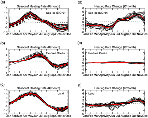
Figure 2. Seasonal heating rate by surface type. Climatological Arctic (60 N–90 N) seasonal heating rate (month-to-month; K*month−1) for the end of the 20th (solid lines) and 21st (dashed lines) centuries projected by CMIP5 historical and RCP8.5 simulations, respectively, for individual CMIP5 models (black lines) and their ensemble mean (red lines) for (a) sea ice, (b) oceanic, and (c) land grid points. The difference between corresponding dashed and solid lines in (a)–(c) is given by (d)–(f), respectively.
Download figure:
Standard image High-resolution imageStratifying the seasonal heating rate  by surface type shows a similar seasonal structure between sea ice (figure 2(a)) and land (figure 2(c)) but a different seasonal structure for ocean (figure 2(b)). We find that sea ice grid points exhibit the largest
  values relative to the other surface types (figures 2(d)–(f)). Despite exhibiting a similar
  seasonal structure to land in the historical simulation, sea ice grid points have a more pronounced seasonal
  pattern than land. During fall and winter, the seasonal heating rate for sea ice increases at ∼twice the rate as that of land in the ensemble average (∼4 K month−1 vs. ∼2 K month−1). Ice-free ocean exhibits small
  values year-round due to its large thermal inertia and smaller increase in net surface energy flux (Dwyer et al
2012, Boeke and Taylor 2018). Since sea ice grid points experience the most pronounced seasonal warming pattern, largest warming, and greatest changes in their seasonal heating rate, we will focus on these grid points.
values year-round due to its large thermal inertia and smaller increase in net surface energy flux (Dwyer et al
2012, Boeke and Taylor 2018). Since sea ice grid points experience the most pronounced seasonal warming pattern, largest warming, and greatest changes in their seasonal heating rate, we will focus on these grid points.
Considering the summer-to-winter transition, figure 2(d) shows an increase in the seasonal heating rate reflecting a slowdown in the background cooling rate of sea ice grid points. Evidence for the strong link between maximum winter warming and the cooling rate reduction is provided by the high and statistically significant spatial correlations for all models (0.88 for the ensemble); the positive correlations in table 1 between  in fall to early winter and the winter warming maximum imply that grid boxes with greater winter warming also possess a larger slowdown in seasonal cooling rate throughout the model ensemble. The high correlation is expected as summer warming does not vary much spatially, such that a greater slowdown of the cooling rate from summer-to-winter indicates a more rapid growth of the fall and winter warming signal and ultimately a larger warming maximum.
Table 1. Spatial correlations between variables for Arctic sea ice grid boxes.
| Model |
 (SOND) vs (SOND) vs  (Max) (Max) |
 (SOND) vs (SOND) vs  (SOND) (SOND) |
 (SON) vs (SON) vs  (SON) (SON) |
 (SON) vs (SON) vs  (SON) (SON) |
 (SON) vs (SON) vs  (SON) (SON) |
|---|---|---|---|---|---|
| ACCESS1.0 | 0.90 | −0.86 | N/A | N/A | −0.79 (−0.81) |
| ACCESS1.3 | 0.91 | −0.89 | N/A | N/A | −0.87 (−0.87) |
| CCSM4 | 0.93 | −0.95 | 0.97 | −0.32 (−0.73) | −0.35 (−0.80) |
| CMCC-CESM | 0.91 | −0.66 | 0.12 | 0.47 (0.47) | −0.71 (−0.71) |
| CMCC-CMS | 0.90 | −0.83 | 0.24 | 0.17 (0.17) | −0.87 (−0.87) |
| CMCC-CM | 0.89 | −0.73 | 0.17 | 0.40 (0.39) | −0.78 (−0.79) |
| CNRM-CM5 | 0.92 | −0.92 | 0.92 | −0.72 (−0.72) | −0.81 (−0.82) |
| CanESM2 | 0.92 | −0.97 | 0.98 | −0.92 (−0.92) | −0.97 (−0.97) |
| GISS-E2-H-CC | 0.71 | −0.78 | N/A | N/A | 0.34 (0.04) |
| GISS-E2-H | 0.76 | −0.83 | N/A | N/A | 0.40 (0.13) |
| GISS-E2-R-CC | 0.80 | −0.67 | N/A | N/A | −0.21 (−0.21) |
| GISS-E2-R | 0.80 | −0.70 | N/A | N/A | −0.28 (−0.28) |
| HadGEM2-AO | 0.86 | −0.44 | N/A | N/A | −0.51 (−0.54) |
| HadGEM2-CC | 0.92 | −0.97 | N/A | N/A | −0.82 (−0.86) |
| HadGEM2-ES | 0.90 | −0.96 | N/A | N/A | −0.84 (−0.86) |
| IPSL-CM5A-LR | 0.92 | −0.84 | 0.96 | −0.67 (−0.68) | −0.74 (−0.74) |
| IPSL-CM5A-MR | 0.93 | −0.83 | 0.98 | −0.70 (−0.70) | −0.72 (−0.72) |
| IPSL-CM5B-LR | 0.84 | −0.63 | 0.93 | −0.53 (−0.55) | −0.65 (−0.68) |
| MIROC-ESM-CHEM | 0.89 | −0.97 | N/A | N/A | −0.92 (−0.92) |
| MIROC-ESM | 0.87 | −0.97 | N/A | N/A | −0.90 (−0.90) |
| MIROC5 | 0.92 | −0.95 | 0.96 | −0.80 (−0.81) | −0.87 (−0.89) |
| MPI-ESM-LR | 0.87 | −0.93 | N/A | N/A | −0.89 (−0.89) |
| MPI-ESM-MR | 0.90 | −0.94 | N/A | N/A | −0.92 (−0.92) |
| MRI-CGCM3 | 0.80 | −0.59 | 0.93 | −0.42 (−0.53) | −0.40 (−0.53) |
| MRI-ESM1 | 0.79 | −0.61 | 0.95 | −0.45 (−0.57) | −0.45 (−0.59) |
| NorESM1-ME | 0.95 | −0.86 | 0.96 | −0.44 (−0.82) | −0.44 (−0.89) |
| NorESM1-M | 0.96 | −0.88 | 0.96 | −0.43 (−0.80) | −0.46 (−0.87) |
| Ensemble Mean | 0.88 | −0.82 | 0.79 | −0.38 (−0.49) | −0.61 (−0.70) |
Values in parenthesis are for grid boxes with total thickness <5 m. a Indicates a model with no snow depth output, so total thickness is just indicative of the sea ice thickness.
A key question becomes what is the underlying cause of these heating rate changes? We hypothesize that both effects are tied to the decline in sea ice cover and thickness that increases the thermal inertia of the surface and the conductive heat flux reaching the sea ice surface from the warmer ocean below.
3.2. Contributions to the seasonal Arctic surface heating rate
The strong connection between the change in the seasonal heating rate and the Arctic surface warming pattern points to the need to understand the changes to the seasonal heating rate. Therefore, we quantify the individual contributions to  . Using the mosaic approach, the Ts of a sea ice grid box is given by the weighted average of the two surface types,

After differentiating with respect to time, the heating rate is given by

where SST is sea surface temperature and Ts,ice is sea ice surface temperature. Applying a first-order Taylor series expansion to the change of equation (2) between the current and future climates yields

The expression in equation (3) decomposes  into contributions from changes in SIC, Ts,ice, SST, and their respective seasonal rates of change. The results in figure 3 are the average of the forward and backward applications of the first order Taylor expansion. Figure 3 depicts only 14 of the 27 models, as only 14 of the models output Ts,ice.

Figure 3. Contributions to the seasonal heating rate change. (a) Total seasonal heating rate change (K*month−1) given by the sum of (b)–(f), where the dashed red line is the actual ensemble mean change of the seasonal heating rate. Contributions to the seasonal heating rate change by the (b) sea ice concentration change (term I), (c) change of the sea ice surface seasonal heating rate (term II), (d) change of the sea surface seasonal heating rate (term III), (e) change in the seasonal rate of change of sea ice concentration (term IV), and (f) change in the temperature difference between the sea surface and sea ice surface (term V). Results for individual CMIP5 models are given by the black lines, while the ensemble mean is given by the red lines. Done for Arctic (60 N–90 N) sea ice grid points.
Download figure:
Standard image High-resolution imageThe decomposition depicts the model-simulated  accurately with a small residual as indicated by the close match between the ensemble mean
  (dashed red line in figure 3(a)) and the sum of the diagnosed terms (solid red line in figure 3(a)). The analysis reveals that the seasonal heating rate changes due to
  SIC (term I) and
  (term II) are the most important contributors to
  . Both contribute about equally to the positive
  during fall (SON) reaching rates of +2 K month−1 in October and November (ensemble mean; figures 3(a)–(c)). However, unlike term II, the duration of the positive contribution by term I extends into early winter. Both terms also contribute to the decrease of the seasonal heating rate seen from spring-to-summer, but the term II contribution is larger and lasts longer.
Since changes in  occur due to changes in net surface energy flux and effective surface heat capacity (see supplementary text) the contributions of individual terms indicate which factors are more important. Term I indicates a shift in weight from the sea ice seasonal heating rate,
  , to the SST seasonal heating rate,
  , due to the decline in sea ice concentration. The greater effective heat capacity of the ocean surface relative to that of sea ice (see supplementary text) causes
  to have a muted seasonal cycle relative to
  (figure S1). Therefore, term I represents an increase in the thermal inertia of the Arctic surface as sea ice concentration declines, which explains the decrease in the amplitude of
  (figure 2(a)), consistent with Dwyer et al (2012).
Hahn et al (2022), hereafter referred to as H22, demonstrated that the increase in effective surface heat capacity due to sea ice loss in idealized model simulations can singularly reproduce the seasonal Arctic warming pattern. Therefore, the greater the areal shift from sea ice to ocean (i.e. term I) the larger the increase in  during fall and winter. The statistically significant spatial anti-correlations for all models (−0.82 ensemble mean; table 1) are evidence that greater reductions in sea ice concentration result in a greater increase of
  during fall to early winter (SOND) even at the grid box scale. During spring and summer, the thermal inertia increase reduces
  but the impact is smaller, as the decline in sea ice concentration is less than in fall and winter (figure S2).
The importance of the  contribution (term II) to
  during fall is corroborated by the statistically significant spatial correlations between
  and
and  for the available models (0.79 ensemble mean; table 1); the exceptions are the CMCC models, which are substantial outliers, removing these models increases the ensemble mean correlation to ∼0.95. The
  seasonal pattern should primarily be driven by changes in the net surface energy flux for sea ice portions of a grid box (S3), as the effective heat capacity of sea ice is not expected to vary substantially; although, small effective heat capacity changes can occur due to changes in the sea ice thickness (SIT) and snow cover.
Figure 4 summarizes changes in the surface energy budget terms for sea ice grid boxes. The surface energy budget changes show increases in upward sensible and latent heat fluxes and upward LW fluxes (figures 4(a)–(c)) during fall and winter, which cool the surface, as well as an increase in downward LW fluxes (figure 4(d)) that warm the surface. Overall, the net change in the surface energy budget (figure 4(f)) is negative indicating a stronger surface cooling in fall and winter, inconsistent with the increase of  and
and  (figures 3(a), (c)).
  , however, is the seasonal heating rate change only over the sea ice portion of sea ice grid boxes, while the net surface energy flux changes in figure 4 represent the entire sea ice grid box. This means the net surface energy flux change over the sea ice portion of the sea ice grid boxes should be positive, even though the net surface energy flux change over the entire sea ice grid box is negative. The inconsistency is likely due to the different surface energy flux changes over the remaining sea ice, sea-ice loss, and ocean portions of an individual sea ice grid box (S5). For example, the increase in latent and sensible heat fluxes should be larger over the sea-ice loss portion of the grid box than over the portions where sea ice and ocean persist. The available CMIP5 output, however, does not allow us to differentiate the surface energy flux changes over the remaining sea ice, sea-ice loss, and ocean portions of an individual grid box. Furthermore, the net surface energy flux calculation does not include the impact of changes in ocean heat transport, oceanic heat conduction through the sea ice that reaches the surface, or latent heat due to sea ice melt. Due to these limiting factors, we cannot unambiguously attribute which surface energy flux changes are responsible for
  . However, we can provide plausible explanations of
  through physical reasoning and concomitant data that backs up the physically based arguments.

Figure 4. Surface energy budget changes. Changes in (a) sensible heat flux, (b) latent heat flux, (c) upward longwave flux, (d) downward longwave flux, (e) net downward shortwave flux, and (f) the net energy flux (sum of (a)–(e)) at the surface for individual CMIP5 models (black lines) and the ensemble mean (red lines) for Arctic (60 N–90 N) sea ice grid points. Units: W*m−2.
Download figure:
Standard image High-resolution imageThe increase of  during fall (SON) is likely due in part to the increase of heat conduction from the ocean to the sea ice surface, which can be a snow surface if snow covered. Though we are unable to directly evaluate the impact of changes in heat conduction through the sea ice, we can indirectly determine its impact through its dependence on sea ice plus snow thickness (i.e. the total thickness). During fall, thicker sea ice not only insulates the atmosphere from the warmer ocean below but also the sea ice surface. A decrease of total thickness in the future leads to increased oceanic heat conduction through the sea ice (Persson et al
2017) providing a large positive contribution to the net surface energy flux change (Manabe and Stouffer 1980). During fall, grid points with greater reductions in total thickness generally exhibit a greater increase of
during fall (SON) is likely due in part to the increase of heat conduction from the ocean to the sea ice surface, which can be a snow surface if snow covered. Though we are unable to directly evaluate the impact of changes in heat conduction through the sea ice, we can indirectly determine its impact through its dependence on sea ice plus snow thickness (i.e. the total thickness). During fall, thicker sea ice not only insulates the atmosphere from the warmer ocean below but also the sea ice surface. A decrease of total thickness in the future leads to increased oceanic heat conduction through the sea ice (Persson et al
2017) providing a large positive contribution to the net surface energy flux change (Manabe and Stouffer 1980). During fall, grid points with greater reductions in total thickness generally exhibit a greater increase of  , as indicated by their spatial anti-correlation (−0.38 for the ensemble mean; table 1). Not all models output snow depth (snow depth is only available for 19 models), but this is not an issue as the correlation analysis with SIT alone is nearly the same with a slight degradation (i.e. snow depth impact is small, not shown). Hereafter, when discussing SIT, we implicitly mean total thickness for models that output snow depth.
Once again, the CMCC models are extreme outliers; unlike any other model, they display positive correlations. Removing these models improves the negative ensemble mean correlation (−0.58). Above a certain thickness the sea ice surface is effectively insulated from the ocean below, such that reductions in thickness do not increase heat conduction to the sea ice surface until the thickness drops below the threshold. If we limit the correlation analysis to grid points with monthly-mean total thickness less than 5 m, then the spatial anti-correlation increases in magnitude to −0.49 (−0.71 if we exclude the CMCC models).
As previously noted, the  is only available for 14 models. However, SIT is available for all 27 models and can act as a proxy for the relationship between
  and
and  during fall, particularly for the other 13 models. The spatial correlation between
  and the change in a SIT is high as expected (−0.61 for the ensemble mean; table 1). Limiting the analysis to grid points with monthly-mean SIT less than 5 m increases the magnitude of the ensemble mean correlation to −0.70, providing credence to the argument that the increase in heat conduction from the ocean to the sea ice surface as sea ice thins is a contributing factor to the increase of
  during fall. The GISS models show the worst correlations, some even exhibiting positive correlations; we found unphysical grid-box values of SIT (over 1000 m), suggesting issues with their SIT output. Removing the GISS models from the ensemble mean improves the negative correlation between
  and ΔSIT from −0.70 to −0.80. We note that the spatial correlation between
  and ΔSIT is high for the CMCC models, unlike that with
  . This suggests possible issues with their Ts,ice output or other factors contribute to the high spatial correlation between
  and ΔSIT.
The decrease of  during spring to early summer, on the other hand, is attributed to the additional latent heat energy from snow and sea ice melt. This is consistent with studies that attribute the lack of summer warming to melt (Manabe and Stouffer 1980, Serreze et al
2009).
during spring to early summer, on the other hand, is attributed to the additional latent heat energy from snow and sea ice melt. This is consistent with studies that attribute the lack of summer warming to melt (Manabe and Stouffer 1980, Serreze et al
2009).
The seasonal heating rate change due to  (term III) is small because of the large thermal inertia of the ocean, thus the seasonal heating rate of the SST portion of a sea ice grid box changes little. The seasonal heating rate changes due to
  (term IV) and
  (term V) are the Taylor expansion of the change in the third term on the right-hand side of (2); this term, which corresponds to the change in the multiplication of the seasonal growth and melt rate of sea ice concentration with the within-grid box sea ice temperature and SST difference
  , contributes little to the change in the seasonal heating rate (not shown). This makes sense as the seasonal growth and melt rate of sea ice cover will be larger when sea ice is thinner; thinner sea ice tends to have a smaller surface temperature difference relative to the sea surface. On the other hand, when sea ice is thick the surface temperature difference relative to the sea surface tends to be large, but the seasonal growth and melt rate are smaller for thicker sea ice. Either situation results in a multiplication with a relatively small value that limits the magnitude of this term and its corresponding change. The non-negligible magnitudes (∼2 K month−1) of terms IV and V in winter months are therefore artifacts of the mathematical decomposition that when considered jointly offset as expected.
3.3. Surface air temperature coupling
The surface air temperature displays the same seasonal Arctic warming pattern (figure S3(a)) as the surface skin temperature ( ) and exhibits a very similar change to its seasonal heating rate (figure S3(b)). Unlike
  , the surface air temperature change cannot be explained by a change in the surface air heat capacity and thermal inertia. The similarities, however, are not surprising since the surface skin and air temperatures are tightly coupled through latent and sensible heat fluxes and thermal-radiative coupling (e.g. Sejas and Cai 2016). The
  and
and  are generally greater (in magnitude) than their respective counterparts for surface air, particularly in fall and winter, indicating the coupling between the two is driven by the surface warming. Since the seasonal cooling from summer to winter slows more for the surface skin than surface air temperature, the surface-to-air temperature difference increases, which leads to stronger upward sensible and latent heat fluxes in fall and winter (figures 4(a) and (b)). This upward latent and sensible heat flux increase contributes to the large fall/winter Arctic surface air temperature warming. Additionally, the warmer surface skin temperatures enhance the upward LW radiation emitted by the Arctic surface (figure 4(c)), warming the surface air through enhanced absorption in the lower atmosphere. It is through these increases in upward energy flux, in regions of sea ice loss, that the warming signal of the surface is imprinted to the lower atmosphere.
3.4. Inter-model spread
All CMIP5 models exhibit maximum Arctic warming in winter. Though the timing of maximum warming is in general agreement among CMIP5 models, the degree of warming differs greatly, ranging from ∼9 K to ∼23 K (monthly mean). In the previous sections, we showed that seasonality of Arctic warming is fundamentally connected to the changes in the seasonal heating rate ( ), which are due to the increase in effective heat capacity of the Arctic surface, as the sea ice cover loss shifts the surface type from a low (sea ice) to a high (ocean) heat capacity surface, and the change in the seasonal heating rate of the sea ice surface (
 ). Within this context, we explore the influence of these terms on the inter-model warming spread.
Figure 5(a) shows a strong and significant correlation (r = 0.92) between  in fall to early winter (SOND) and the maximum monthly-mean surface warming, indicating CMIP5 models with a greater drop in their fall/early winter cooling rate experience a larger maximum warming. The inter-model spread in sea ice cover loss during fall to early winter also correlates significantly with both the spread in the warming maximum (r = −0.83; figure 5(b)) and
  (r = −0.71; figure 5(c)), consistent with table 1. This suggests that the inter-model spread in sea ice cover loss during fall to early winter impacts the inter-model warming spread mainly through its influence on
  . The net surface energy flux changes (for the available terms) have a negative inter-model correlation (r = −0.47) with
  during fall to early winter (figure 5(d)), which is the opposite sign one would expect if greater net surface energy flux changes were responsible for greater increases in
  .
.

Figure 5. Inter-model correlations. Correlations across models between (a) SOND seasonal heating rate changes and maximum winter warming, (b) SOND sea ice concentration changes and SOND seasonal heating rate changes, (c) SOND sea ice concentration changes and maximum winter warming, (d) SOND net surface energy flux changes and SOND seasonal heating rate changes, (e) SOND seasonal ice heating rate changes and SOND seasonal heating rate changes, and (f) SON seasonal ice heating rate changes and SON seasonal heating rate changes. Computed for Arctic (60 N–90 N) sea ice grid points.
Download figure:
Standard image High-resolution imageUnlike the inter-model spread in ΔSIC, the spread in  does not correlate well with
  in fall to early winter (figures 5(e) and (f)), nor with the maximum warming. This indicates that even though
  is important to explaining the physics of
  , it is not an important contributor to the inter-model spread. This result highlights the role of the shift from low-to-high heat capacity as sea ice declines in both the physics of the seasonal Arctic warming pattern and the large inter-model warming spread.
4. Discussion
Unlike most studies that assert surface energy flux changes explain the seasonality of Arctic surface warming, our analysis indicates that the thermal inertia change due to the transition from sea ice to sea water is an important factor driving the asymmetric seasonal pattern of Arctic surface warming and its dependence on surface type, consistent with Robock (1980), Dwyer et al (2012), and H22. Our results suggest that surface energy flux changes also play an important role, as the increase in heat conduction from the ocean to the sea ice surface and the increase in downward LW fluxes contribute to an increase of the fall surface heating rate, while the enhanced melting in spring and summer reduces the warming amplitude from winter to summer.
The thermal inertia feedback represents a change in the surface temperature sensitivity to energy fluxes that impacts the seasonal magnitude of Arctic warming. The thermal inertia feedback mainly operates via changes in sea ice concentration. Therefore, any climate feedback (SAF, clouds, etc) that affects the evolution of sea ice cover can influence the character of the thermal inertia feedback. In consequence, changes in surface energy fluxes and thermal inertia are inextricably linked. Based upon the importance of fall/early winter thermal inertia changes on the projected winter warming maximum, surface energy budget perturbations due to climate feedbacks in fall are important for the thermal inertia feedback by delaying the sea ice freeze onset. For instance, recent studies indicate that an increase in Arctic low clouds, in response to sea ice reductions, has the potential to enhance downward LW radiation at the surface and delay fall freeze onset. In addition, an increase in downward LW radiation due to enhanced fall/early winter heat and moisture transport by the atmosphere could also delay fall sea ice freeze onset (Lee et al 2017, Luo et al 2017, Boeke and Taylor 2018, Hegyi and Taylor 2018). Thus, the representation of clouds and atmospheric energy transports in fall/early winter could play a significant role in modulating the seasonal warming pattern through the thermal inertia feedback by delaying fall sea ice freeze onset. Similarly, oceanic heat transports have also been found to influence the timing of fall sea ice freeze onset (Steele et al 2008).
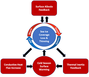
The thinning and loss of sea ice cover connects many of the key processes responsible for the seasonal expression and magnitude of Arctic warming. Both the thermal inertia feedback and SAF are triggered by the loss of sea ice cover. Thinner sea ice is more susceptible to melting in spring and summer, while also allowing for greater heat conduction from the ocean to the surface in fall. Considering an arbitrary starting point, the SAF in spring and summer increases the ocean heat content, which delays fall freeze onset (i.e. reduces ice cover) and thins sea ice during fall and winter. The drop in sea-ice cover increases the thermal inertia of the surface, while thinner sea ice increases the heat conduction from the ocean to the surface. These changes reduce the seasonal cooling rate leading to maximum warming in early winter. Thinner and warmer sea ice in fall/winter promotes thinner sea ice in spring and summer. The strong interseasonal connection for SIT between the cold and warm seasons is corroborated by the high interseasonal spatial correlation all CMIP5 models have for  SIT (0.92 ensemble mean). Thinner sea ice is more vulnerable to melting-out and uncovering the darker ocean underneath leading to a larger SAF in spring and summer. The increased melting combined with the thermal inertia increase reduces the seasonal warming rate during spring and summer leading to a warming minimum in summer. As long as a positive external forcing is applied, the interseasonal interaction between the SAF, thermal inertia feedback, and conductive heat flux (shown schematically in figure 6) continues until no sea ice remains and represents an amplifying (i.e. positive) feedback loop that not only establishes the seasonal Arctic warming pattern but is a dominant contributor to Arctic warming amplification.
Figure 6. Sea ice loss interseasonal interaction. Schematic showing the interseasonal interaction between the SAF, thermal interia feedback, and conductive heat flux that not only is induced by the decline in sea ice coverage and thickness but causes further sea ice loss and amplifies cold season Arctic warming. Arrows from the warm to cold season and vice-versa illustrate the reinforcing interseasonal nature of the interaction that amplifies cold season warming under the presence of an external forcing.
Download figure:
Standard image High-resolution image
Yang et al (2022) reported a positive feedback loop between asymmetric melt onset and end variations and summer sea ice melt. Specifically, summer sea ice melt delays freeze onset, which further increases summer sea ice melt, leading to a greater delay of freeze onset. This positive feedback loop is consistent with the feedback loop induced by the interaction between the SAF, thermal inertia feedback, and conductive heat flux. Furthermore, the delay of freeze onset is accompanied by a delay in the timing of the Arctic warming maximum (Yang et al 2022). Previous studies have also demonstrated the shift in the timing of the Arctic warming maximum from early to late winter as sea ice declines (Dai et al 2019, Liang et al 2022). Consistent with our results, Dai et al (2019) showed that the magnitude of Arctic warming is connected to the magnitude of sea ice decline. As sea ice declines in the cold season, the thermal inertia increases, which decelerates the typical seasonal cooling that occurs during fall and winter, leading to a progressively greater delay in the freeze onset and timing of the Arctic warming maximum. Once sea ice disappears further Arctic warming and amplification are greatly reduced in the presence of continued greenhouse forcing (Dai et al 2019).
The interaction between the SAF, thermal inertia feedback, and conductive heat flux explains why the SAF, which is only effective in spring and summer, correlates well with the fall to early winter decline in sea ice cover (−0.92) and increase in seasonal heating rate (0.65), and the winter warming maximum (0.84; figure S4). It also explains why fixing surface albedo to a constant, while allowing the sea ice concentration to decline, greatly reduces the magnitude of Arctic warming (Hall 2004); however, the seasonal Arctic warming pattern remains about the same (figure 2 in Hall 2004) since the sea ice cover loss and thinning caused by the greenhouse forcing and other climate feedbacks would still increase the thermal inertia, heat conduction from the ocean to the sea-ice surface, and melting. By enhancing the decline in sea-ice cover and thickness the SAF amplifies Arctic warming and enhances the difference between the maximum and minimum warming in winter and summer, respectively, through its impact on the aforementioned processes.
5. Summary and conclusions
Under greenhouse gas forcing, CMIP5 models robustly project a pronounced seasonal Arctic warming pattern that is minimum in summer and maximum in winter. Sea ice loss regions are primarily responsible for the seasonal warming pattern, accounting for 56% (ensemble mean) of the winter warming in the Arctic (60 N–90 N) even though they account for only 44% (ensemble mean) of the area. The transition from a low (sea ice) to a high effective heat capacity surface (ocean) as sea ice declines plays a key role in establishing the pronounced seasonality displayed by sea ice loss regions. Land regions exhibit a similar seasonal warming structure, but less pronounced. Henry and Vallis (2021) indicate the smaller heat capacity of land and the nonlinearity of the temperature dependence of surface LW emission establish the seasonal warming pattern over land. Ice-free ocean regions, on the other hand, display relatively muted warming with very little seasonality due to their larger effective heat capacity (Dwyer et al 2012, Henry and Vallis 2021). Effective heat capacity is therefore an important surface property key to determining the seasonality and magnitude of the warming in the Arctic.
Utilizing a simple idealized model and conducting model sensitivity experiments, H22 also demonstrated that the alteration of effective heat capacity due to melting sea ice is a crucial driver of the seasonal Arctic warming pattern. Furthermore, H22 corroborates the conclusion that the increase in conductive heat flux with sea ice thinning contributes to the amplification of winter warming. Their modeling approach allows them to isolate the process contributions key to the seasonality of Arctic warming, highlighting the fundamental impact effective heat capacity changes have on the seasonality of Arctic warming. Alternatively, this study arrives at similar conclusions by analyzing an array of fully coupled global climate models (GCMs) using mathematical decomposition to isolate key contributors accompanied with statistical analysis. While this study is unable to disentangle and isolate process contributions as neatly as the idealized model simulations used in H22, it demonstrates that even in fully coupled GCMs the importance of effective heat capacity change due to sea ice loss on the seasonal Arctic warming pattern holds. Moreover, not only does this study indicate that the main results of H22 hold across CMIP5 models but also shows that the inter-model spread in the effective heat capacity change strongly contributes to the inter-model Arctic warming spread. The studies are therefore complementary, arriving at similar conclusions using different approaches.
Our analysis clearly points to the importance of sea-ice loss, both in coverage and thickness, on the amplitude and seasonal structure of Arctic warming. Differences in the location, magnitude, and timing of sea-ice loss among models will strongly impact the inter-model warming spread. Thus, an improved understanding and modeling of the factors that influence sea ice cover and thickness (e.g. sea ice physics, ocean mixed layer depth, surface energy budget, atmospheric variability etc) are needed to produce more reliable simulations of Arctic warming. For example, a recent study (Massonnet et al 2018) shows that CMIP5 inter-model differences in sea ice loss can be traced to differences in the simulation of seasonal growth and melt in the present climate, which relate to the background SIT. Another study (Boeke and Taylor 2018) found that climate models simulate a wide range of present-day values and projected changes in mixed layer depth in the Arctic that impact the effective heat capacity of the surface. We see great potential for using observations of effective heat capacity, sea ice concentration and thickness, and fall freeze onset to constrain projected winter warming and reduce uncertainty in projected AA.
Acknowledgments
S A Sejas' research was supported by an appointment to the NASA Postdoctoral Program at the NASA Langley Research Center, administered by Universities Space Research Association under contract with NASA P C Taylor is supported by the NASA Radiation Budget Science Project and by the NASA Interdisciplinary Studies Program grant NNH12ZDA001N-IDS. We acknowledge the World Climate Research Programme's Working Group on Coupled Modelling, which is responsible for CMIP, and we thank the climate modeling groups (listed in table S1 of this paper) for producing and making available their model output. For CMIP the U S Department of Energy's Program for Climate Model Diagnosis and Intercomparison provides coordinating support and led development of software infrastructure in partnership with the Global Organization for Earth System Science Portals. S A Sejas conceived the idea for this study, downloaded the data, and performed the calculations. S A Sejas and P C Taylor discussed the results throughout the whole process and were responsible for the writing of the manuscript.
Data availability statement
The data that support the findings of this study are openly available at the following URL/DOI: https://data.ceda.ac.uk/badc/cmip5/data/cmip5/.
Supplementary Information (5.6 MB DOCX)