

Abstract
Observational records of meteorological and chemical variables are imprinted by an unknown combination of anthropogenic activity, natural forcings, and internal variability. With a 15-member initial-condition ensemble generated from the CESM2-WACCM6 chemistry-climate model for 1950–2014, we extract signals of anthropogenic ('forced') change from the noise of internally arising climate variability on observed tropospheric ozone trends. Positive trends in free tropospheric ozone measured at long-term surface observatories, by commercial aircraft, and retrieved from satellite instruments generally fall within the ensemble range. CESM2-WACCM6 tropospheric ozone trends are also bracketed by those in a larger ensemble constructed from five additional chemistry-climate models. Comparison of the multi-model ensemble with observed tropospheric column ozone trends in the northern tropics implies an underestimate in regional precursor emission growth over recent decades. Positive tropospheric ozone trends clearly emerge from 1950 to 2014, exceeding 0.2 DU yr−1 at 20–40 N in all CESM2-WACCM6 ensemble members. Tropospheric ozone observations are often only available for recent decades, and we show that even a two-decade record length is insufficient to eliminate the role of internal variability, which can produce regional tropospheric ozone trends oppositely signed from ensemble mean (forced) changes. By identifying regions and seasons with strong anthropogenic change signals relative to internal variability, initial-condition ensembles can guide future observing systems seeking to detect anthropogenic change. For example, analysis of the CESM2-WACCM6 ensemble reveals year-round upper tropospheric ozone increases from 1995 to 2014, largest at 30 S–40 N during boreal summer. Lower tropospheric ozone increases most strongly in the winter hemisphere, and internal variability leads to trends of opposite sign (ensemble overlaps zero) north of 40 N during boreal summer. This decoupling of ozone trends in the upper and lower troposphere suggests a growing prominence for tropospheric ozone as a greenhouse gas despite regional efforts to abate warm season ground-level ozone.
Export citation and abstract BibTeX RIS
1. Introduction
With its relatively short lifetime ranging from days in some surface regions to several weeks in the free troposphere, tropospheric ozone is highly variable in space and time (Logan 1985). Long-term trends in tropospheric ozone observations can arise from changes in air pollutant emissions and in climate, as well as from internal variability ('noise'), particularly over small spatial scales (Hawkins and Sutton 2009, 2011, Kirtman et al 2013). The influence of internal variability, however, is often overlooked when interpreting observed trends in atmospheric composition. Large ensemble simulations in physical climate models (Kay et al 2015) demonstrate that low frequency climate variability can amplify or mask anthropogenically forced local trends in North American surface temperature, even over a 50 year period (Deser et al 2012a, 2012b, 2014). Below, we introduce a novel perspective to interpret observed tropospheric ozone trends through the lens of initial condition chemistry-climate model ensembles. Our analysis strongly supports earlier findings that tropospheric ozone has continued its rise in response to human activities during recent decades, while revealing that the magnitude—and in some cases the sign—of locally observed tropospheric ozone trends are shaped by internal variability.
The Tropospheric Ozone Assessment Report (TOAR) compiled and analyzed multi-decadal tropospheric ozone observations to examine variability and trends in tropospheric ozone distributions (Chang et al 2017, Schultz et al 2017, Gaudel et al 2018, Tarasick et al 2019). These observations include continuous measurements at remote ground-level sites (e.g. Oltmans et al 2013), from approximately weekly ozonesondes (e.g. Logan 1994, Thompson et al 2021), from routine commercial aircraft (e.g. Petzold et al 2015), and retrieved from satellite instruments (e.g. Ziemke et al 2019). We focus here on trends derived from observational datasets that are available for nearly a quarter century and are best suited to comparison with monthly mean ozone from chemistry-climate models: measurements aboard commercial aircraft (Gaudel et al 2020); the Ozone Monitoring Instrument/Microwave Limb Sounder (OMI/MLS) and Total Ozone Mapping Spectrometer (TOMS) tropospheric column ozone satellite products (Ziemke et al 2019), and remote ground-level stations previously shown to sample a wide range of trends in the boundary layer, though these surface measurements do not necessarily reflect trends in the free troposphere (Cooper et al 2020).
The capacity to conduct century-long climate simulations with tropospheric chemistry offers new opportunities to assess model representation of trends, as we present below. Prior evaluation of chemistry-climate models with ozone observations at selected long-term observational sites spurred debates over whether these models are fit-for-purpose, as summarized by TOAR (Young et al
2018). Newer work demonstrates that the models represent salient features of spatial and temporal variability including decadal changes despite an excessive north-to-south gradient and discrepancies with trends derived from individual measurement sites (Young et al
2018), and notes some shortcomings of the statistical approaches applied to interpret observed trends (Cooper et al
2020, Chang et al
2021). A sparse set of lower tropospheric and surface ozone measurements suggest northern hemispheric increases of 30%–70% since the middle of the 20th Century; improved observations increase confidence in tropospheric ozone trends since the mid-1990s, with estimated increases of 2%–7% and 2%–12% per decade in sampled regions of the northern mid-latitudes and in the tropics, respectively, with more limited sampling leading to lower confidence in southern hemispheric trends (Gulev et al
2021). Novel analysis of clumped oxygen isotopes of molecular oxygen places an upper bound of 40% on the tropospheric ozone increase since the pre-industrial period (Yeung et al
2019), lending additional observation-derived support to the 109  25 Tg increase over this period simulated with chemistry-climate models assessed by the Intergovernmental Panel on Climate Change (IPCC) (Szopa et al
2021).
25 Tg increase over this period simulated with chemistry-climate models assessed by the Intergovernmental Panel on Climate Change (IPCC) (Szopa et al
2021).
Earlier work seeking to interpret observed tropospheric ozone trends and evaluate their representation in chemistry-climate models lacked a rigorous approach to quantify the role of internal variability. This shortcoming is of particular concern when comparing a small set of model simulations with observations at the scale of an individual site or small region of the troposphere. Now computationally feasible, tropospheric chemistry-climate model initial-condition ensembles, such as those described in this paper, provide a means to begin quantifying the influence of internal variability on observed trends in tropospheric ozone. This approach also enables a re-framing of atmospheric chemistry model evaluation. For atmospheric chemistry models driven by or nudged to reanalysis (observed) meteorology, it is appropriate to ask 'Does the model capture the observed trends?'. Applying this question to a chemistry-climate model, however, fails to recognize a role for internal variability in causing simulated trends to diverge from an observed trend, even if the simulated trend is fully consistent with the real-world forcings. When evaluating a chemistry-climate model, the question becomes, 'Does the observed trend fall within the range of those simulated by the model ensemble?'. The larger the chemistry-climate model ensemble, the stronger the statistical basis for drawing robust conclusions as to the role of internal variability on measurements. Note that the ensembles included here are forced by the same combination of greenhouse gas concentrations and anthropogenic air pollutant emissions, whereas a fuller ensemble could include uncertainty in these forcings, or separate their roles via parallel 'single forcing' ensembles (e.g. Deser et al 2020b).
Small ensembles have previously been used to explore the influence of internal climate variability on tropospheric ozone trends. For example, Lin et al (2014) demonstrated that observed long-term ozone trends at Mauna Loa are attributable to decadal climate variability. Lin et al (2015a) and Lin et al (2015b) also found a role for internal variability on Western U.S. surface and tropospheric ozone, including a higher frequency of deep stratospheric ozone intrusions during La Niña events. Barnes et al (2016) mapped globally the spatial and seasonal variations in the length of time needed to reliably detect surface ozone trends driven by anthropogenic emissions in the presence of internal variability. Polvani et al (2019) used a 13-member climate model ensemble with interactive stratospheric ozone chemistry to demonstrate that internal variability overwhelms the forced signal from large volcanic eruptions over Eurasia in winter. For the Aerosol Chemistry Model Intercomparison Project (AerChemMIP) under the Coupled Model Intercomparison Project Phase 6 (CMIP6), multiple international modeling groups generated simulations with interactive tropospheric chemistry (Collins et al 2017). These new simulations broadly capture observed ozone distributions and trends (Griffiths et al 2021), and we use them below to provide context for our analysis of observed regional and site-level tropospheric ozone trends with an initial-condition ensemble from a single model.
Below, we describe a CESM2-WACCM6 full chemistry historical ensemble, transferring methods pioneered with 'large-ensemble' simulations in the physical climate community (Deser et al 2012a, 2020a, 2020b) to atmospheric chemistry. We examine trends since 1950 on the basis of earlier work showing that the largest increases in tropospheric ozone occurred after 1950 (Shindell et al 2006), when anthropogenic emissions of ozone precursors rose sharply (Hoesly et al 2018). The initial-condition ensemble simulates a range of trends that might have been observed if climate had varied differently. Our approach to interpreting trends and variability in tropospheric ozone (section 2) serves as an illustrative example for applying initial-condition ensembles to separate forced trends (signal; section 3) driven by anthropogenic emissions or episodic volcanic eruptions from internal variability (climate noise). We demonstrate that observed free tropospheric ozone trends generally fall within the range of the CESM2-WACCM6 ensemble, and that the CESM2-WACCM6 ensemble is not only within the range of the broader CMIP6 chemistry-climate historical ensembles, but also captures observed tropospheric ozone trends at least as well as other current generation chemistry-climate models (section 4). We then apply the initial-condition CESM2-WACCM6 ensemble to interpret tropospheric column ozone trends derived from available satellite instruments (section 5), and identify tropospheric regions and seasons where anthropogenic signals are strongest such that forced tropospheric ozone trends can be detected most rapidly (section 6) before discussing our conclusions in the context of a future outlook (section 7).
2. Approach
2.1. Chemistry-climate initial-condition ensemble simulations for 1950–2014
Model Description. Our analysis centers on a 15-member ensemble generated with the Community Earth System Model version 2—Whole Atmosphere Community Climate Model version 6 (CESM2-WACCM6) from 1950 to 2014. With its inclusion of a modal representation of aerosol microphysics linked to detailed gas-phase chemistry that includes several secondary organic aerosol precursors, CESM2-WACCM6 is a major advance in the tropospheric chemistry complexity represented in a fully coupled climate model (Gettelman et al 2019, Tilmes et al 2019, Danabasoglu et al 2020, Emmons et al 2020). The model ingests the CMIP6 Historical anthropogenic (Hoesly et al 2018) and biomass burning (van Marle et al 2017) emissions. A step change in the variability of biomass burning emissions when the satellite record becomes available (van Marle et al 2017) has been shown to produce spurious extratropical Northern Hemisphere warming from increased absorption of solar radiation due to a thinning cloud field (Fasullo et al 2022), which could affect tropospheric ozone trends estimated from these simulations.
Initial Condition Ensemble. Three CESM2-WACCM6 ensemble members, available from the NCAR contribution to CMIP6, were launched from a long preindustrial control simulation and then followed the Historical emissions and forcing trajectories until 2014 (Danabasoglu et al 2020). We select January 1, 1950 from these three simulations for use as initial conditions (ocean, sea ice, atmosphere, land), and slightly perturb atmospheric temperature (O∼ 10−14 K) separately to produce four additional members, following Deser et al (2012a) and Kay et al (2015), for a total of 12 new ensemble members. Each ensemble member differs from the others only in its initial conditions of the climate state, thereby offering a unique estimate of one possible combination of the atmospheric chemistry and climate responses to anthropogenic and natural forcing plus internal variability from 1950 to 2014. By averaging over 'climate noise' resulting from different initial conditions, the ensemble mean offers a best estimate of the 'true' changes occurring in response to anthropogenic (and natural) forcing. Anthropogenic forcing includes changes in air pollutant emissions, greenhouse gasses, stratospheric ozone depleting substances, and land-use change associated with human activities. The range across the ensemble provides a measure of internal variability, or what might have been observed if climate varied in a different way under the exact same forcing scenario. In a perfect model with a sufficient ensemble size to average out climate noise, one could unambiguously attribute the portion of observed trends due to anthropogenic change versus internal variability. With our imperfect model, we can nevertheless make progress towards this goal.
Evaluation of Model Climate. The model has previously been evaluated for several climate variables as part of CESM2 development and CMIP6 activities. The simulated CESM2-WACCM6 climate is similar to CESM2-CAM6, capturing salient features of observed 20th century climate, such as temperature trends throughout the atmospheric column (Gettelman et al 2019, Danabasoglu et al 2020). The model is one of the best at representing northern hemisphere atmospheric circulation including storm tracks, blocking events, stationary waves, the North Atlantic Oscillation, and jet streams, although westerlies tend to be too strong over Europe, and easterlies too strong over Africa (Simpson et al 2020).
Tropospheric Ozone Evaluation. Prior work evaluating tropospheric ozone with ozonesondes and airborne data composites reveals that the model generally captures observed abundances around the globe to within 25% (Emmons et al 2020). Griffiths et al (2021) previously reported decadal mean tropospheric ozone burdens averaged over the three CESM2-WACCM6 ensemble members in the CMIP6 archive of 282 and 310 Tg for 1975–1984 and 1995–2004, respectively, lower than the ranges across four other models (307–355 and 327–387 Tg). The CESM2-WACCM6 ensemble mean tropospheric ozone burden of 317 ± 3 Tg (standard deviation is calculated from the individual 1998–2002 years from all 15 ensemble members) is lower than observational estimates of 335 ± 10 Tg (Wild 2007) using a 150 ppb ozone tropopause definition (Text S1). The tropospheric ozone burden estimates increase to 328 ± 4 Tg for CESM2-WACCM6 and 352 ± 30 Tg from observations (Wild 2007) using a thermal lapse rate tropopause (Text S1). The CESM2-WACCM6 estimates are also slightly lower than other more recent observational estimates (Young et al 2018) but are within the wide range of estimates from satellite products (∼250–350 Tg; Griffiths et al 2021) and the range of 347 ± 28 Tg assessed from available observations and models (Szopa et al 2021). In contrast to this mean state evaluation, our analysis below centers on identifying patterns of change while accounting for the role of internal climate variability when comparing models and measurements. Griffiths et al (2021) found that while the CMIP6 models simulate different mean tropospheric ozone burdens, they capture observation-based trends of 0.70 ± 0.15 Tg yr−1 from an ozonesonde derived product and 0.83 ± 0.85 Tg yr−1 from an ensemble of satellite products since 1997 (CMIP6 models: 0.82 ± 0.13 Tg yr−1).
CMIP6 chemistry-climate models. To place our findings from CESM2-WACCM6 in the context of current generation models, we draw on five additional fully coupled chemistry-climate models that submitted historical simulations to the CMIP6 archive as part of AerChemMIP (Collins et al 2017). These models include GISS–E2–1 (four different configurations; Bauer et al 2020, Kelley et al 2010, Miller et al 2021, NASA GISS 2018, 2019), UKESM1–0–LL (two configurations; Archibald et al 2020a, Sellar et al 2019, Tang et al 2019), BCC-ESM1 (Wu et al 2020, Zhang et al 2018), GFDL-ESM4 (Dunne et al 2020, Krasting et al 2018), MRI-ESM2-0 (Yukimoto et al 2019) previously described and evaluated with tropospheric ozone observations by Griffiths et al (2021) and Turnock et al (2020). Combining these CMIP6 simulations with our CESM2-WACCM6 ensemble yields a 73-member multi-model ensemble. Table S1 briefly describes each of the five models and gives the number of ensemble members with each model configuration. CESM2-WACCM6 is excluded from the CMIP6 ranges in the comparisons shown below. We account for internal variability by interpreting overlapping inter-model ensemble ranges as consistency across models.
2.2. Selected observations for regional ozone trend analysis
Surface Measurements. We select surface observations measured at the six sites from Cooper et al (2020) with the longest continuous records made with reliable measurement techniques (Tarasick et al 2019). Measurements began in different years, and we use all available years through 2014 when the CMIP6 historical simulations end. These include monthly median values from four baseline NOAA Global Monitoring Laboratory (GML) sites, plus two mid-latitude sites: Barrow Atmospheric Baseline Observatory (ABO), Alaska (observations began in 1973); Mauna Loa ABO, Hawaii (1973; plus 1957–1959); American Samoa ABO, South Pacific (1976); South Pole ABO, Antarctica (1975, plus 1961–1963); Hohenpeissenberg, Germany (1971) and Cape Grim, Tasmania (1982). The observations were carefully screened by Cooper et al (2020) to select for well-mixed atmospheric conditions (usually nighttime at mountaintop sites and daytime for low elevation sites), which are most suitable for comparison to coarse resolution global models. We also include measurements available for a few years in the 1950s and 1960s at Mauna Loa and the South Pole, respectively, from a Regener Automatic instrument. To compare with these measurements, we convert site altitude to pressure (assuming a surface pressure of 1000 hPa and a scale height of 7.5 km) and sample the model monthly mean ozone values at the vertical level containing the corresponding pressure, from which we construct annual means for each ensemble member. Annual mean anomalies are calculated from the observations and from each individual ensemble member by subtracting the multi-year average taken from the beginning of the observed record until 2014. We calculate trends following the methods of Cooper et al (2020) applied to monthly mean ozone concentrations. Trends and their associated uncertainties are estimated by the generalized least squares (GLS) method, with harmonic components incorporated to account for the seasonal variation and an autoregressive-1 adjustment applied to the 2-sigma uncertainty of the trend (Chang et al 2021).
Columns derived from IAGOS aircraft measurements. We use multi-decadal regional-scale tropospheric ozone trends derived from routine sampling by the IAGOS commercial aircraft (IAGOS; (Thouret et al
1998, Petzold et al
2015) compiled for the Tropospheric Ozone Assessment Report (Gaudel et al
2018) plus additional updates (Gaudel et al
2020; regions shown in figure S1). This analysis is heavily weighted towards the northern hemisphere, with tropospheric column sampling possible only where the instrumented commercial flights ascend and descend regularly at airports. Observed trends are calculated since 1994 in all regions except for Persian Gulf and Malaysia/Indonesia, which are since 1998 and 1995, respectively. The IAGOS data were analyzed separately for the free and full tropospheric columns (Gaudel et al
2020), such that differences between the free and full tropospheric columns are attributable to ozone trends in the boundary layer. We compare trends in median ozone derived from IAGOS measurements (figure 2 of Gaudel et al
2020) to the annual mean trends simulated by each individual ensemble member. The observed trends are calculated as the slope from the GLS applied to the monthly means (accounting for seasonality). For each region and year, model monthly mean ozone fields are sampled for 1994–2014, except for the Persian Gulf and Malaysia/Indonesia regions, which we sample since 1998 and 1995, respectively, for consistency with the observational record. Gaudel et al (2020) report trends through 2016, but our simulations end in 2014, so there is a slight mis-match in the time period sampled. We select all vertical grid cells within the bounding latitude–longitude boxes surrounding the IAGOS flight tracks in each region (figure S1), where the top edge pressure  250 hPa, and where the bottom edge pressure is
  700 hPa (free tropospheric column; note that there is a mis-match for northern South America for which the free troposphere has a lower boundary of 600 hPa in Gaudel et al (2020)) or 950 hPa (full tropospheric column). Capping the tropospheric column at 250 hPa will not capture the full extent of the troposphere in the tropics and may include some of the lower stratosphere in winter at high latitudes. Discrepancies in trends derived from the monthly IAGOS data versus monthly mean model ozone may also result from the different temporal sampling frequency. For each ensemble member and year, the monthly regional average column ozone mixing ratio (ppb) is deseasonalized by subtracting the multi-year monthly average ozone. The slope from a simple linear regression applied to the monthly anomalies is then calculated for each ensemble member.
Tropospheric Column Ozone from Satellite. We examine annual mean tropospheric column ozone trends, previously described by Ziemke et al (2019), within 10° latitude bands. Multi-decadal satellite records of tropospheric ozone columns are available in the tropics (30 S–30 N) from 1979 to 2005, derived from the convective cloud differential method applied to total column ozone retrieved from the TOMS instrument. We also compare tropospheric column ozone trends over the tropics and mid-latitudes (60 S–60 N) for the last decade of the historical simulations (2005–2014) derived from the OMI total column and MLS stratospheric columns (Ziemke et al 2019). For consistency with the methods used to derive the observed trends, we use a tropical tropopause height of 100 hPa to define the CESM2-WACCM6 tropospheric column ozone for comparison with TOMS (available in the tropics only) and the thermal lapse rate definition for comparison with the OMI/MLS tropospheric column ozone product. We note the potential for discrepancies to arise from different temporal sampling frequencies in addition to the variations in instrument sensitivity with altitude as we do not apply any vertical weighting functions (averaging kernels) to the simulated ozone fields. For all tropospheric columns and burdens we calculate temporal trends as the slope of the ordinary least squares fit.
3. Extracting forced signals in global tropospheric ozone trends from internal variability: 1950–2014
Long-term positive trends in the global annual mean tropospheric ozone burden arise in each individual ensemble member (thin black lines in figure 1), indicating significance relative to internal variability. The range across these individual members can be as much as 5–10 Tg in any given year. This range is a measure of the variations in the tropospheric ozone burden arising solely from internal variability. Following methods established in the climate modeling community, we interpret the ensemble mean (thick lines in figure 1), which averages over variations due to internal variability, as a best estimate of the tropospheric ozone response to external forcing. In this section, we interpret trends and variations in the ensemble mean.
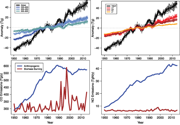
Figure 1. The global annual mean tropospheric ozone burden increased (black, repeated in both top panels) from 1950 to 2014 with ozone precursor emissions, such as global CO (bottom left) and NOx (bottom right) from anthropogenic activities (blue) and biomass burning (dark red). In the top panels, thin lines show the 15 individual CESM2-WACCM6 ensemble members and thick lines show the ensemble mean anomaly in each year, separated into northern (dark blue), tropical (light blue), and southern latitudes (aquamarine; top left) and upper (red), middle (dark red), and lower troposphere (gold; top right). Anomalies are calculated annually with respect to a 1970–1990 reference period.
Download figure:
Standard image High-resolution imageOver the 20th century, long-term trends are primarily driven by growth in anthropogenic tropospheric ozone precursor emissions, as illustrated for annual emissions of ozone precursors nitrogen oxides (NOx ) and carbon monoxide (CO) from anthropogenic sources and biomass burning in figure 1. Global concentrations of methane, a major precursor to tropospheric ozone also rose throughout this period except for a pause from the late 1990s into the mid-2000s (not shown; Meinshausen et al 2017). Anthropogenic climate change may also affect tropospheric ozone trends over this period, but cannot be isolated from the role of rising precursor emissions without additional sensitivity simulations. Short-term ensemble mean excursions of a few years reflect responses to natural forcings, which include sporadic volcanic eruptions as well as the biomass burning events in the historical emissions (figure 1), which are applied to all ensemble members.
The CESM2-WACCM6 global annual ensemble mean tropospheric ozone (thick black line in figure 1) increases by over 80 Tg from 1950 to 2014. For comparison, the IPCC 6th Assessment Report (AR6) assessed observational and model evidence to estimate an increase in the tropospheric ozone burden of 109  25 Tg from 1850 to present-day, with medium confidence (Szopa et al
2021). The increases in the first two decades (1950–1969) are dominated by the northern hemisphere (20–90 N), where the ozone burden rises at twice the rate of the tropics (20 S–20 N). During this period, the tropical growth rate approaches three times that of the southern hemisphere (20 S–90 S; figure 1 and table S2). In contrast, the growth rates in tropospheric burdens are much more similar in all three hemispheric regions from 1990 to 2009 (figure 1 and table S2).
25 Tg from 1850 to present-day, with medium confidence (Szopa et al
2021). The increases in the first two decades (1950–1969) are dominated by the northern hemisphere (20–90 N), where the ozone burden rises at twice the rate of the tropics (20 S–20 N). During this period, the tropical growth rate approaches three times that of the southern hemisphere (20 S–90 S; figure 1 and table S2). In contrast, the growth rates in tropospheric burdens are much more similar in all three hemispheric regions from 1990 to 2009 (figure 1 and table S2).
The tropospheric ozone increases roughly follow the rise in global anthropogenic NOx emissions (figure 1) as well as methane, which have previously been shown to be the dominant precursors for global annual mean tropospheric ozone (Fiore et al 2002, Shindell et al 2005). Global anthropogenic CO emissions (figure 1) grew sharply prior to 1970, with average emissions more or less flattening out over the most recent decades (and declining from 1990 to 2009; table S2), although biomass burning emissions in some years more than offset the decline in anthropogenic CO emissions (figure 1). We calculate tropospheric ozone burden anomalies relative to a 1970–1990 reference period (figure 1), selected as the middle two decades of the time series when the tropospheric ozone burden is not rising rapidly (figure S2). The larger tropospheric ozone burden trends before 1970 than during the 1970–1990 reference period directly follow emission trends of anthropogenic NOx (and CO) emissions (figure 1; table S2). From 1990 to 2009, however, the total tropospheric ozone burden rises more steeply than in the 1970–1989 period, even though the growth in global anthropogenic NOx emissions is smaller (0.47 Tg N y−1 versus 0.68 Tg N y−1 in 1950–1969; table S2). The rate of increase in the upper tropospheric ozone burden doubles in 1990–2009 relative to earlier periods (0.89 versus 0.38–0.39 Tg O3 y−1; table S2). Zhang et al (2016) previously identified that 1980–2010 increases in tropospheric ozone were driven in part by the shift in anthropogenic NOx emissions towards more tropical latitudes (see figure 5 of Gaudel et al 2020), where abundant radiation enables efficient ozone production throughout much of the year. Zhang et al (2021) showed that emission growth in East Asia from 1980 to 2010 contributes strongly to increasing upper tropospheric ozone, with smaller contributions from South Asia and rising methane concentrations, outweighing the decreasing influence from North American and European emissions over this period. These findings, together with figure 1, imply a role for convective lofting of ozone and precursors to the free troposphere, where ozone production is more efficient and the lifetime is longer than near the surface, in driving the overall increase in the tropospheric ozone burden (Berntsen et al 1996, Naik et al 2005, Sauvage et al 2007). Increasing aircraft NOx emissions over this period may also play role in the overall burden increase (Wang et al 2022). The ozone increases in the lower troposphere are largest in the first two decades of the simulation, more in line with the overall trends in global anthropogenic emissions (table S2).
Short-term excursions in tropospheric ozone timed with changes in anthropogenic emissions are also evident from figure 1. For example, the 1970s downturns align with temporary decreases in global anthropogenic NOx and CO emissions. A natural, volcanic forcing signal is evident in tropospheric ozone, which produces downturns in the otherwise increasing tropospheric ozone trends timed with eruptions from Mount Agung in 1963, El Chichón in 1982, and Mount Pinatubo in 1991. These eruptions imprint a particularly strong signal on annual mean tropospheric ozone at mid-latitudes, presumably as ozone depletion in the lower stratosphere decreases stratosphere-to-troposphere ozone transport (e.g. Lin et al 2015b). The southern hemisphere responds most strongly to Mount Agung (Bali, Indonesia) whereas the northern hemisphere responds most strongly to Mount Pinatubo (Philippines).
In addition to volcanic eruptions, sporadic biomass burning events are another source of forced variability in these simulations, even though in reality these events are tied closely to the specific meteorological situation (discussed further in section 7). For example, the 1997–1998 El Niño event triggered extreme emissions (Duncan et al 2003, van Marle et al 2017), during which CO emissions from biomass burning are estimated to exceed those from anthropogenic sources (figure 1). During this event, the tropospheric ozone burden rose sharply by over 20 Tg O3 globally from the anomalous low associated with the Pinatubo eruption to the anomalous high associated with the 1997–1998 El Niño event. While anomalously high stratosphere-to-troposphere transport has also been identified during this event (Zeng and Pyle 2005), we do not expect this source of tropospheric ozone to emerge as a forced response in the initial-condition ensemble as the climate state of the tropical Pacific will vary across members (i.e. they do not all simulate an El Niño in 1997–1998). We underscore that the biomass burning emissions are driving these simulations in an 'offline' sense, and are not consistent with the simulated climate state of the equatorial Pacific.
4. Interpreting observed tropospheric ozone trends with initial-condition ensembles
4.1. The CESM2-WACCM6 ensemble versus observed regional trends
We show below that the observed trends in annual mean tropospheric ozone, both at selected long-term monitoring sites (five baseline sites and one representative of regional-scale pollution in Western Europe; figure 2) and in the full and free tropospheric columns (to 250 hPa; see section 2.2) over regions with frequent, routine sampling by commercial aircraft (figure 3), usually fall within the range of trends simulated by the CESM2-WACCM6 model ensemble. Gaudel et al (2020) note that longer observational records are less likely to be influenced by internal variability, but the role of internal variability on ozone trends has not been quantified, and is challenging to extract from short, sparse observational records (McKinnon et al 2017). We show below that two decades of observations is insufficient to eliminate the role of internal variability on observed regional free tropospheric ozone trends.
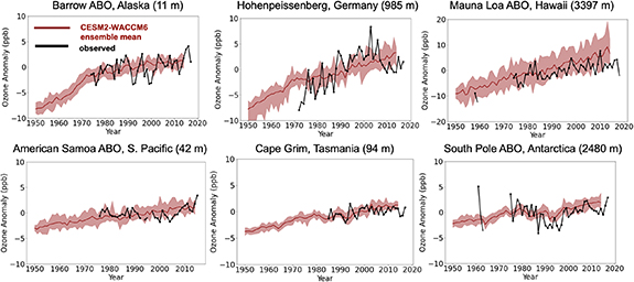
Figure 2. Anomalies in annual mean ozone observed at six measurement sites with the longest observational records (black lines) generally fall within the range of those simulated by 15 CESM2-WACCM6 ensemble members sampled at measurement locations (maroon shading; thick line is the ensemble mean). Observed annual means are only included if at least 6 months are available within a given year; filled circles denote years with at least ten monthly mean values available. Each panel states the site location and elevation. ABO denotes Atmospheric Baseline Observatory.
Download figure:
Standard image High-resolution image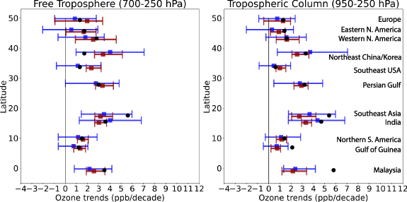
Figure 3. A wide range of regional tropospheric ozone trends in recent decades arises in the free troposphere (left) and tropospheric column (right) from internal variability (maroon; CESM2-WACCM6). Trends are calculated starting in 1994 for all regions except for the Persian Gulf and Malaysia, which start in 1998 and 1995, respectively. The observed free tropospheric ozone trends (black circle) derived from the IAGOS ozone measurements all fall within the multi-model ensemble range (blue; CMIP6 models, not including CESM2-WACCM6), with the exception of the two regions closest to the equator where emission increases are likely underestimated. See section 2.2 for methods and figure S1 for region definitions.
Download figure:
Standard image High-resolution imageThe observed ozone anomalies (see section 2.2 for methods) generally fall in the inter-ensemble range sampled at the six selected long-term monitoring sites (figure 2). All CESM2-WACCM6 ensemble members simulate positive trends from 1950 to 2014 at all sites, with ensemble mean values ranging from 0.6 ppb decade−1 at both South Pole ABO and American Samoa (ensemble range at both sites is 0.5–0.7 ppb decade−1) to 2.5 ppb decade−1 (ensemble range of 2.3–2.8 ppb decade−1) at Mauna Loa ABO (hereafter MLO; table S3). Over the shorter record lengths when measurements are available, at least one model ensemble member simulates a trend of similar magnitude to those derived from the observations, except at American Samoa where the observation-derived trend is not significant (table S3). All members of the CESM2-WACCM6 ensemble simulate positive trends (p
 0.05, ≪0.01 for most sites and time periods; table S3) except at Barrow ABO since 1982.
At five of the six sites in figure 2, the observed year-to-year variability exceeds that of the ensemble range. At MLO, however, the range across the CESM2-WACCM6 ensemble members fully encompasses the measurements, which we attribute to the careful observational sampling of the free troposphere by Cooper et al (2020) to isolate large-scale conditions represented in a global model. The model skill at MLO suggests that the other sites are influenced by local processes not resolved with coarse model grid cells.
In contrast to the continued rise of the model ensemble mean tropospheric ozone at MLO, the observed trend flattens around the turn of the century. Observed versus simulated tropical mid-troposphere temperature trends in CMIP6 models show a similar pattern, with weaker observed trends attributed to multidecadal variability, specifically a decadal cooling of the equatorial Pacific Ocean (Po-Chedley et al 2021). This tropical Pacific multi-decadal variability and an associated shift in atmospheric circulation and ozone transport has previously been shown to obscure the signal from rising Asian emissions on springtime ozone trends at MLO (Lin et al 2014). Figure 2 suggests an extension of this influence to the annual mean trend, and the same phenomenon may explain the smaller observed anomalies relative to those modeled in the last decade of the simulation at Cape Grim and American Samoa ABO.
As was evident from the global tropospheric ozone burden in figure 1, some anomalies in figure 2 are clearly forced as they occur in the ensemble mean. For example, the model ensemble mean simulates a step change in the ozone rate of increase at Barrow ABO, Alaska in the early 1970s, just as measurements were established, such that the trend since observations began is about half that over the full time period (table S3). The influence of the El Chichón and Mt. Pinatubo volcanic eruptions on ozone measured at the South Pole, and to a lesser extent Cape Grim, emerges in the ensemble mean anomalies. The Agung eruption is also evident in the pre-measurement period at Cape Grim and the South Pole ABO. While the model ensemble mean suggests that the decreasing trend observed at Hohenpeissenberg since 1995 (Cooper et al 2020) reflects internal variability rather than a forced trend, this low-elevation site near the center of Western Europe is likely sensitive to regional decreases in ozone precursor emissions that may not be well captured in the model. Our analysis illustrates how an initial-condition ensemble can be used to assess the extent to which observed trends reflect external forcings (e.g. ozone precursor emission trends, volcanic eruptions) that emerge in the model ensemble mean trend, versus internally arising variability, which differs across ensemble members.
We next examine the tropospheric column trends derived from the IAGOS aircraft measurements over 11 world regions in the context of trends derived from the model ensemble. Figure 3 shows the ensemble mean slope of the CESM2-WACCM6 ensemble (maroon squares) and the range in slopes derived from individual ensemble members (maroon bars span the minimum to maximum trend) as compared to the observed trend (black circle). For 8 and 7 out of 11 regions with long-term sampling by aircraft, the observed free and total, respectively, tropospheric ozone column trends fall within the range simulated by the 15-member CESM2-WACCM6 ensemble (figure 3).
Free tropospheric ozone trends of 1–2 ppb decade−1 over the Southeast U.S.A. and Northeast China/Korea are overestimated by all CESM2-WACCM6 ensemble members, with the smallest trend simulated by any ensemble member ∼1 ppb decade−1 higher than observed (figure 3). The total tropospheric column trends, however, do overlap in these regions, suggesting some compensation in the model between changes in the lowermost troposphere versus aloft. In contrast, the model ensemble underestimates both the >5 ppb decade−1 free and total tropospheric ozone column trend over Southeast Asia by nearly 2 ppb decade−1. When the full tropospheric column is considered, ozone trends are also underestimated by CESM2-WACCM6 over the Gulf of Guinea by ∼1 ppb decade−1 and Malaysia by over 2 ppb decade−1. The approximate doubling of the observed trends in the full versus free tropospheric columns is due to large ozone increases in the boundary layer over these regions (Gaudel et al 2020). While this single model ensemble is still rather small, these findings suggest an error in the ozone precursor emission changes in these regions, which we revisit in sections 4.2 and 5.
Our general finding that the individual model ensemble members simulate changes in ozone that span the range of those observed, both at the long-term surface sites and in the free tropospheric regions sampled by IAGOS, lends confidence to using the ensemble to attribute observed signals. The simulated changes in ensemble mean tropospheric ozone with time offer the best estimate of the influence from the combined historical anthropogenic and natural forcings, which are imposed identically across all ensemble members. From 1994 to 2014, ensemble mean tropospheric ozone trends increase over all 11 regions (maroon squares in figure 3), typically by 1–3 ppb decade−1 in CESM2-WACCM6.
The individual CESM2-WACCM6 ensemble members provide a novel perspective on the range of tropospheric ozone trends that might have been observed under different contributions from internal variability. Even though each ensemble member is driven with identical anthropogenic ozone precursor emissions, we find ozone trends of opposite sign simulated across the ensemble over Europe, ranging from −1 ppb decade−1 to +3 ppb decade−1 in the free troposphere. The inter-ensemble range in figure 3 illustrates that even with two decades of observations, trends require careful interpretation if they are to be accurately attributed to driving factors, such as changes in ozone precursor emissions and climate given the inherent 'climate noise'. Note that this inter-ensemble range is an estimate of the uncertainty associated with internal variability, which is relevant for attributing a trend to a specific process (e.g. anthropogenic emissions, volcanic eruptions). Uncertainty in the trend magnitude derived from a single ensemble member or from observations, usually conveyed by a confidence interval, reflects uncertainty in the the derived trend itself, arising from the range of possible values under least-squares minimization.
In figure 4, we use the initial-condition ensemble to further illustrate the potential for internal climate variability to produce trends of different signs and magnitudes under the same historical scenario. Figure 4 shows annual mean lower tropospheric ozone trends over 20 year (left) and 10 year (right) periods in the CESM2-WACCM6 simulations. While some common patterns such as the decreases over South America and the increases over Southeast Asia emerge in all four panels, different signed trends occur elsewhere, including over the U.S.A., northern Eurasia, much of Africa, the equatorial Pacific, and the North Atlantic, even when 20 year trends are considered. We emphasize that these differences occur even though all ensemble members are driven by the exact same greenhouse gases and tropospheric ozone precursor emissions from anthropogenic sources and biomass burning. In ensemble member 15, slight differences in initial conditions are sufficient to produce zero-to-positive trends for the 1995–2014 period over much of the U.S.A. and Europe even though ozone precursor emissions decline in these regions. Figure 4 also implies a need to consider internal variability when we are interpreting observed trends, even over multiple decades, as we do not know the relative contributions from the forced signal versus internal variability on the observed record.
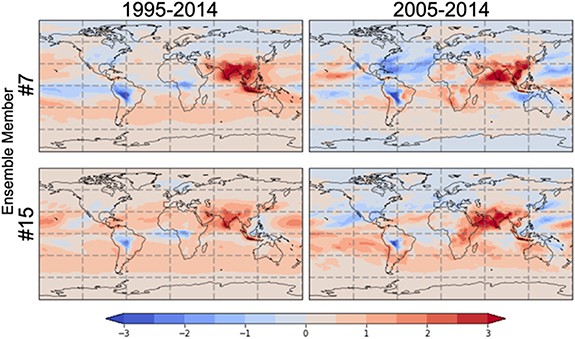
Figure 4. The sign and magnitude of tropospheric ozone trends can vary regionally between individual ensemble members due to different initial conditions even when the greenhouse gas and ozone precursor emissions (anthropogenic and biomass burning) are identical in all ensemble members. Shown are annual mean lower tropospheric (surface to 690 hPa) ozone burden trends (Tg decade−1) over 20 year (1995–2014; left) and 10 year (2005–2014; right) periods in two selected CESM2-WACCM6 ensemble members: #7 (top) and #15 (bottom).
Download figure:
Standard image High-resolution image4.2. Multiple chemistry-climate model ensembles versus observed regional trends
We now extend our analysis of the CESM2-WACCM6 ensemble to the larger CMIP6 chemistry-climate model ensemble. By considering differences across individual model ensembles, we address structural uncertainty: inter-model differences in the simulated responses to the same combination of anthropogenic and natural forcing. Our comparison of this broader set of models with the observed annual mean ozone concentrations at the six long-term measurement sites (figure 5) indicates that CESM2-WACCM6 is often the model closest to the observed concentrations as well as the observed trends (table S3). An exception is Barrow ABO, Alaska, where none capture the observed concentrations, and all neglect the role of tropospheric halogen chemistry (e.g. Barrie et al 1988, Oltmans et al 2012) and CESM2-WACCM6 shows a systematic 5–10 ppb positive bias. Even with a low bias of a few ppb in some years at the South Pole ABO site, CESM2-WACCM6 is closest to the observed concentrations (figure 5). Overall, we find in figure 5 that the differences across models are larger than the differences within a single model ensemble, suggesting a major role for model structural uncertainty in contributing to inter-model differences in tropospheric ozone. In contrast, the range in monthly ozone anomalies across the CMIP6 models nearly always brackets the observed anomalies (figure S3). The CESM2-WACCM6 ensemble annual mean anomalies and concentrations generally fall close to those calculated from the CMIP6 ensemble (figures S3 and 5). Prior to the observational period, and thus outside the reference time period used to calculate anomalies, CESM2-WACCM6 will not encompass the CMIP6-model mean given the wide range in simulated trends at some sites (e.g. Hohenpeissenberg, Cape Grim, and South Pole ABO in figure 5).

Figure 5. Annual mean ozone concentrations observed at six measurement sites with the longest observational records (black) generally fall within the range of those simulated by the CMIP6 model ensemble (colors, one per model configuration; thick line indicates ensemble mean and shading indicates inter-ensemble range). Observed annual means with 10 monthly mean values are shown as filled circles. Each panel states the site location and elevation; note different y-axis ranges. The number of ensemble members for each model is given in table S1.
Download figure:
Standard image High-resolution imageCombining across our CMIP6 and CESM2-WACCM6 simulations yields a 73-member ensemble. Figure 3 shows that none of the models simulates a tropospheric column ozone trend as large as those observed over Asia or the Gulf of Guinea. The CMIP6 model ensemble, however, does envelope the free tropospheric ozone trends. We conclude that simulated boundary layer trends are too small and likely indicate an underestimate of emission growth in these regions. This conclusion is also supported by multi-decadal chemistry-transport model simulations driven by reanalysis ('observed') meteorology compared to not only the IAGOS data, but also to long-term ozonesonde measurements (Christiansen et al 2022, Wang et al 2022).
Over all regions in figure 3, the multi-model CMIP6 ensemble fully brackets the range spanned by the CESM2-WACCM6 ensemble, with the minor exception of the full tropospheric column over Malaysia where at least one CESM2-WACCM6 ensemble member simulates a smaller increase in ozone than any other model. Even though the CMIP6 model ensemble mean trend in tropospheric ozone is positive over all of the regions in figure 3, the inter-ensemble member CMIP6 range indicates that negative tropospheric ozone trends consistent with the historical anthropogenic forcing could have occurred (though with a lower probability) in 6 of the 11 regions, with the possibility of zero trend in the free troposphere over the Persian Gulf. This wider CMIP6 model range incorporates the additional source of uncertainty from different model responses (structural uncertainty) and thus should not be interpreted as indicating that CESM2-WACCM6 under-samples the internal variability in tropospheric ozone trends, although we cannot rule out that possibility with a 15-member ensemble.
If we had similar numbers of ensemble members contributed by each model, we could probe more quantitatively the relative roles of internal variability versus model structural uncertainty in contributing to the overall CMIP6 range of trends. Nevertheless, this existing ensemble of opportunity clearly demonstrates that models differ in their responses over some regions (figures 3, 5 and S3). Single- model ensemble ranges of tropospheric ozone column trends versus the IAGOS data (figure S4) are most separated over the Northeast China/Korea region, where the single-model ensemble mean values range from 1 to 6 ppb decade−1. In contrast, single-model ensemble mean tropospheric column ozone trends are more similar over Malaysia. The UKESM1 and MRI-ESM2 ensembles systematically simulate smaller (or negative) trends in the free tropospheric column over all regions compared to the other models. No single model simulates a range of tropospheric column ozone trends spanning the observed trend over India (figure S4) even though it is encompassed by the full CMIP6 range (figure 3).
Overall, the CESM2-WACCM6 ensemble simulations capture many of the salient features of the observed tropospheric ozone trends in figures 3 and 5. Furthermore, the ensemble mean often falls close to the CMIP6 mean (which does not include the CESM2-WACCM6 simulations), suggesting that conclusions drawn with this model should apply more broadly. With these points in mind, we turn next to explore large-scale trends in tropospheric column ozone averaged over 10° latitude bands with the CESM2-WACCM6 ensemble simulations.
5. Identifying latitudinal variations in tropospheric column ozone trends
Annual mean tropospheric ozone column trends from 1950 to 2014 are positive in each individual ensemble member in every 10° latitude band (figure 6), with the largest growth rates (>0.2 DU y−1) simulated at 20–40 N. The historical (1850–1859 to 2005–2014) CMIP6 multi-model ensemble mean changes in annual mean tropospheric column ozone are also positive across the globe and largest at northern mid-latitudes (Griffiths et al 2021; their figure 10). Models indicate that the tropospheric ozone burden increased most in the latter half of the 20th Century, when anthropogenic emissions rose most rapidly (Shindell et al 2006, Griffiths et al 2021). We compare simulated tropospheric ozone column trends to those derived from the TOMS (1979–2005) and OMI/MLS (2005–2014) satellite instruments, respectively (figure 6). Comparing across panels in figure 6, the stronger influence of internal variability over shorter record lengths (Hawkins and Sutton 2009) manifests as larger relative variability in the trends simulated by individual ensemble members.

Figure 6. Increasing tropospheric column ozone trends (DU y−1) in the latter half of the 20th Century, and comparison to trends derived from the satellite record. Shown are the distribution of trends across the 15-member CESM2-WACCM6 initial-condition ensemble (blue box denotes inter-quartile (25th–75th percentile) range; whiskers denote 2-sigma range) within 10° latitude bands from 1950 to 2014 (top), 1979 to 2005 (middle), and 2005 to 2014 (bottom). Red diamonds denote the satellite-derived trends from TOMS (middle) and OMI/MLS (bottom). Different tropopause definitions are used for consistency with retrieval approaches from TOMS (100 hPa pressure surface) versus OMI/MLS (thermal lapse rate, also used for 1950–2014 period); see also text S1.
Download figure:
Standard image High-resolution imageThe model ensemble also provides a window into the potential for internal variability to influence the trends derived from satellite instruments. While CESM2-WACCM6 trends are positive (0.1–0.2 DU y−1) in the tropics over the 26 year period (1979–2005) observed by TOMS, the satellite-derived trends indicate little change, from weakly negative trends to at most +0.05 DU y−1. The MERRA-2 GMI model also simulated larger positive trends than retrieved from TOMS (Ziemke et al 2019; their figure 4). Our analysis demonstrates that the model-TOMS discrepancies cannot be explained by internal variability alone as none of the ensemble members simulate negative trends, or positive trends as small as those retrieved from TOMS. Future efforts could examine the extent to which differences between the satellite and models in temporal sampling and in the vertical extent of the tropospheric column contribute to this discrepancy.
In contrast, OMI/MLS tropospheric ozone column products, available for the final decade of the historical simulation, generally fall within the inter-ensemble range of the trends derived from CESM2-WACCM6. In the 20 S–10 N and 80–90 S latitude bands, the CESM2-WACCM6 ensemble indicates that trends near zero or even negative could have occurred under the historical forcing scenario. Even in latitude bands where all ensemble members simulate positive trends, the ensemble range can span factors of ∼3–5, implying significant uncertainty in quantifying the magnitude of trends attributable to rising anthropogenic emissions. For example, at 10–20 N, only a single ensemble member captures the OMI/MLS trend, which exceeds 0.2 DU y−1. While the model-observation discrepancy identified from the limited IAGOS regional sampling in the northern tropics (figure 3) may extend more broadly across the latitude band, our inter-ensemble range indicates that internal variability can produce tropospheric column ozone trends with magnitudes spanning nearly a factor of four at this latitude band.
Over the full 65 year simulation period, however, the relatively small inter-ensemble range indicates that we can confidently detect trends of varying magnitudes by latitude. This confidence is evident, for example, from the lack of overlap in the size of the trends at high southern latitudes versus those in the tropics (30 S to 10 N) versus those from 10 to 60 N. Because these trends are similar across all ensemble members, they can be interpreted as the forced signal and more specifically attributed to the long-term anthropogenic forcing (see emission increases in figure 1) over this period.
6. Determining anthropogenic tropospheric ozone trends: Regional and seasonal differences
In this section, we show how the CESM2-WACCM6 initial-condition ensemble can be applied to identify regions and seasons where anthropogenic signals can be detected most readily amidst internal variability, and thereby guide analyses of existing or future observations. We probe the model to examine differences in trends in the upper (380 hPa to tropopause) versus lower (>690 hPa) troposphere, where ozone is of most concern as a greenhouse gas and air pollutant, respectively. We also examine seasonal variations in trends, with the aim of identifying locations and seasons where anthropogenic trends are most detectable in light of internal variability. We focus this analysis on the final two decades of the historical simulation with CESM2-WACCM6, a period when high-quality observations are available, at least at northern mid-latitudes in both the near-surface troposphere from ground-based air quality monitoring networks and other long-term measurement sites, as well as in the upper troposphere from the IAGOS flights.
We summarize the annual mean ozone trends in the lower versus upper troposphere by 10° latitude band in the 15-member CESM2-WACCM6 ensemble from 1995 to 2014 (figure 7, blue boxes). Annual mean ozone increases significantly (2-sigma range does not overlap zero) throughout the lower troposphere south of 50 N from 1995 to 2014. The largest annual mean ozone trends in the lower troposphere occur between 20 and 30 N (ensemble mean of the central trend estimate is 0.027 Tg y−1). Lower tropospheric trends are weakest at higher latitudes, where the 2-sigma range overlaps zero north of 50 N. In the upper troposphere, similar latitudinal patterns occur, with the largest ensemble annual mean trends at 20–30 N of 0.08 Tg y−1, reflecting the increasing anthropogenic NOx emissions at this latitude band (Gaudel et al 2020). All ensemble members simulate positive upper tropospheric ozone trends, with the inter-ensemble range only including zero at the poles. Given the observed seasonal cycles in tropospheric ozone (e.g. Logan 1985), we also examine the 1995–2014 upper and lower tropospheric ozone trends separately for June–July–August (JJA) versus December–January–February (DJF; green versus orange in figure 7). Focusing first on the upper troposphere, we find that at 60–90 S and 70–90 N, the inter-ensemble range of DJF upper tropospheric trends overlaps zero. Over much of the tropics and extratropics (30 S–40 N), trends in JJA are 0.02–0.08 Tg y−1 larger than in DJF, and the seasonal interquartile ranges do not overlap (except slightly at 0–10 S). The largest difference occurs at 20–30 N, where the JJA upper tropospheric trend is ∼2.5 times larger than in DJF. For the 10–40 N latitude bands where these seasonal differences in trends are sufficiently strong as to be readily detectable with the CESM2-WACCM6 ensemble (no overlap in the 2-sigma range in figure 7), we infer that it may also be possible to detect these differences with a careful sampling of IAGOS observations in the upper troposphere, though such analysis is beyond the scope of this paper. Although the region and season definitions in figure 7 differ, Gaudel et al (2020; see their tables S1(a) and (b)) also find larger warm season trends relative to the cold season over Western North America, Northeast China/Korea, Persian Gulf, India, Southeast Asia, and Malaysia/Indonesia, consistent with our interpretation that the simulated seasonal trends in the zonally integrated upper tropospheric ozone burden in figure 7 at least partially reflect emission growth in these convectively active regions.

Figure 7. Seasonal and regional differences in tropospheric ozone trends from 1995 to 2014. Annual mean (blue), December–January–February (DJF; orange) and June–July–August (JJA; green) ozone burden trends are shown in the upper (380 hPa to tropopause; top) and lower (>690 hPa; bottom) troposphere for each 10° latitude band. The box and whiskers depict the 25th–75th and 2-sigma (95% confidence intervals) range, respectively, of the trend diagnosed from the 15 individual CESM2-WACCM6 ensemble members.
Download figure:
Standard image High-resolution image
Turning to the 1995–2014 lower tropospheric ozone trends, we find that DJF and JJA trends separate from each other (no overlapping trends within the interquartile range in figure 7) in all latitude bands outside of the tropical (20 S–20 N) and southern polar (70–90 S) regions. Positive wintertime lower tropospheric ozone trends emerge at all latitude bands. Gaudel et al (2020) also generally find larger lower tropospheric ozone trends in the cold versus warm seasons over most regions sampled by IAGOS (exceptions are Northeast China/Korea, Persian Gulf, Southeast Asia, and India). North of 40 N, summertime lower tropospheric ozone trends overlap zero, with an ensemble mean negative trend at 40–50 N, likely reflecting the influence of anthropogenic emission controls, including those implemented to abate ozone and particle pollution under the U.S. Clean Air Act. Over this period, fossil fuel NOx emissions declined by 25% between 40 and 70 N, but increased by up to 50% at ∼25 N (see figure 5 of Gaudel et al 2020), consistent with the lower tropospheric trends by latitude band in figure 7. Seasonal differences in lower tropospheric ozone trends at northern mid-latitudes during this period have previously been reported (Cooper et al 2012, 2020). The new perspective provided by this initial-condition ensemble confirms that the differences in seasonal trends are robust to internal variability. Figure 7 also indicates, however, that the 20 year period is insufficient to detect a robust downward zonally averaged summertime trend in lower tropospheric ozone due to regional anthropogenic emission reductions, in light of some unknown combination of internal variability plus possible offsetting influences from rising emissions in other regions, including from biomass burning (figure 1). Larger wintertime trends in both hemispheres at least partially reflect the longer lifetime of ozone in this season (e.g. Clifton et al 2020). Ozone produced at lower latitudes can thus impart a stronger signal if exported to higher latitudes (Gaudel et al 2020; Zhang et al 2016).
7. Discussion, conclusions, and future outlook
We examine tropospheric ozone trends from 1950 to 2014 via a new perspective offered by 15-member initial-condition ensemble simulations with a chemistry-climate model (CESM2-WACCM6), supplemented by an additional 58 historical ensemble members generated with five other models contributing to CMIP6. While our ensemble is small with respect to those created by the physical climate modeling community, which often include 40–100 members varying only in their initial conditions (Deser et al 2020a), our intent is to illustrate how chemistry-climate ensemble simulations can be analyzed to identify regions and seasons where anthropogenic signals in tropospheric composition can be detected most readily amidst internal variability. These simulations enable an assessment of uncertainty due to internal variability: the range across trends simulated by individual ensemble members relative to the ensemble mean, forced, trends estimated from a single model. Future work could explore model structural uncertainties, which refer to the differences in model responses when subjected to the same forcings, by examining differences in the individual CMIP6 models that cannot be explained by internal variability.
We find that tropospheric ozone burden increases in the early decades of the simulation are dominated by the northern hemisphere, where ozone precursor emissions increase most rapidly, while the tropical and northern hemispheric growth rates are similar by the last couple decades of the simulation. Zhang et al (2016), (2021) previously found that the 1980–2010 spatial shift in global anthropogenic NOx emissions from northern mid-latitudes to the tropics, especially over South and Southeast Asia, contributed to raising the tropospheric ozone burden. Similarly, a multi-model study found larger ozone production in the northern tropics, especially from 2000 to 2010 when regional NOx emissions rose rapidly (Archibald et al 2020b). When we separate trends into two-decade periods in the lower, middle, and upper troposphere, we find that the most rapid (linear) increases in recent decades occur in the upper troposphere. We infer a role for increases in tropospheric ozone precursors in the tropical latitudes where ozone is efficiently produced throughout the year and, along with precursors, is convectively lofted to the free troposphere where the ozone lifetime is longer, as also pointed out by Zhang et al (2016). Increases in aircraft NOx emissions may play a particularly strong role in the upper tropospheric ozone increases (Wang et al 2022). From 1995 to 2014, upper tropospheric and lower tropospheric trends decouple both in sign, consistent with observations assessed by Gulev et al (2021). Trends also differ by season at northern mid- and high-latitudes where emission controls were implemented to reduce warm-season ground-level ozone.
Even though each ensemble member is driven with identical anthropogenic ozone precursor emissions, we nevertheless find ozone trends of opposite sign simulated across the ensemble over some regions. Our inter-ensemble ranges (figures 3, 4, 6 and 7) illustrate that even two decades of observations are not sufficient to eliminate the role of internal variability on observed regional free tropospheric trends. This inherent 'climate noise' implies that observed trends require careful interpretation if they are to be accurately attributed to driving factors, such as changes in ozone precursor emissions or climate. Given a sufficiently large ensemble and unbiased model such that we have confidence in the quantitative attribution of the ensemble mean trend to the forced signal in the observations, we could interpret the difference between the model ensemble mean trend and the observed trend as the influence of low-frequency climate variability on the observed record.
Earlier work emphasized the dependence of the size of the ensemble upon the signal strength relative to internal variability (Hawkins and Sutton 2009). This signal-to-noise ratio varies with the spatial and temporal scales under consideration. For example, in figure 6, the inter-ensemble range of trends shrinks as we move from one decade (bottom panel) to more than five (top panel).
The initial-condition chemistry-climate model ensembles analyzed here enable us to attribute observed tropospheric ozone changes to global environmental change versus internal variability. Cleanly separating the role of anthropogenic emission changes from natural forcings such as volcanic eruptions, or from feedbacks triggered by anthropogenic climate change would require additional sets of initial-condition ensemble simulations. The role of biomass burning emissions in driving the simulated ozone trends will be important to disentangle in future work given the discontinuity in the emission inventory when satellite data become available (van Marle et al 2017). More generally, since biomass burning emissions are imposed in the historical simulations, they act as a 'forcing' applied identically across ensemble members, leading to coherent short-term variations in tropospheric ozone, including during the 1997–98 El Niño event associated with large Indonesian wildfires (Duncan et al 2003). This model treatment poses a conceptual inconsistency by breaking the link between internal variability and its co-variation with the frequency and intensity of fires in many regions, particularly as fires may be one of the largest feedbacks of changes in climate on atmospheric composition.
We view our study as a first step towards a new approach to connecting atmospheric chemistry in models and observations. Analyzing existing observational records through the lens of initial-condition ensembles may offer new insights into the interpretation and attribution of trends, as we have illustrated above. As discussed in Deser et al (2020a), many additional applications of initial-condition chemistry-climate model ensembles are possible, such as building statistical samples of events that are 'rare' or not sampled in existing observational records from model ensembles, or dynamically downscaling individual events for in-depth process studies. Finally, identifying tropospheric regions where the signals from anthropogenic perturbations are strongest and meteorological variability weakest can guide deployment of future observing systems targeting rapid detection of anthropogenic change.
Acknowledgments
A M F gratefully acknowledges useful discussions with Clara Deser, Dan Horton and other members of the U S CLIVAR Large Ensemble Working Group and participants in the 2019 workshop, and with Ben Santer. L M P is funded by NSF Award #1914569 from the US NSF to Columbia University. O R C, K L C and A G were supported by the NOAA Cooperative Agreement with CIRES, NA17OAR4320101. IAGOS has been funded by the European Union projects IAGOS-DS (Design Study) and IAGOS-ERI (European Research Infrastructure). The IAGOS database is supported in France by AERIS (www.aeris-data.fr, last access: 30 June 2022). We acknowledge the strong support of the European Commission, Airbus and the airlines (Deutsche Lufthansa, Air France, Cathay Pacific, Iberia, China Airlines and Hawaiian Airlines) that carry the IAGOS equipment, partner institutions of the IAGOS Research Infrastructure (FZJ, DLR, MPI, and KIT in Germany; CNRS, Météo-France, and Université Toulouse III Paul Sabatier in France; the University of Manchester in the UK), and national agencies in Germany (BMBF), France (MESR), and the UK (NERC).
Data availability statement
The data that support the findings of this study are openly available at the following URL/DOI: https://hdl.handle.net/1721.1/145676.
Supplementary data (0.4 MB PDF)