

Abstract
High fractions of variable renewable electricity generation have challenged grid management within the balancing authority overseen by the California's Independent System Operator (CAISO). In the early evening, solar resources tend to diminish as the system approaches peak demand, putting pressure on fast-responding, emissions-intensive natural gas generators. While residential precooling, a strategy intended to shift the timing of air-conditioning usage from peak-demand periods to cheaper off-peak periods, has been touted in the literature as being effective for reducing peak electricity usage and costs, we explore its impact on CO2 emissions in regional grids like CAISO that have large disparities in their daytime versus nighttime emissions intensities. Here we use EnergyPlus to simulate precooling in a typical U.S. single-family home in California climate zone 9 to quantify the impact of precooling on peak electricity usage, CO2 emissions, and residential utility costs. We find that replacing a constant-setpoint cooling schedule with a precooling schedule can reduce peak period electricity consumption by 57% and residential electricity costs by nearly 13%, while also reducing CO2 emissions by 3.5%. These results suggest the traditional benefits of precooling can be achieved with an additional benefit of reducing CO2 emissions in grids with high daytime renewable energy penetrations.
Export citation and abstract BibTeX RIS
1. Introduction
Increasing penetrations of variable renewable power generators can challenge reliable grid management, particularly in electricity grids where there is a temporal mismatch between peak renewable energy generation and peak electricity demand. Managing the large ramping requirements needed to quickly bring generation resources online to transition from periods of low net demand (which often align with high renewable energy penetration) to periods of high net demand can be difficult [1]. (Note: here we define net demand as total demand minus variable renewable energy generation [2].) This phenomenon is already evident in California's Independent System Operator (CAISO) territory, where high penetrations of solar power have created challenging grid conditions commonly referred to as the 'duck curve'. The duck curve refers to CAISO's diurnal net load curve, which is characterized by (1) a deep daytime net load dip (i.e., the 'belly' of the duck) caused by high solar photovoltaic penetration and relatively low demand, and (2) a steep increase in net load that occurs as the sun sets in the early evening and CAISO simultaneously enters its evening peak load period [3].
To accommodate the large generation ramping requirements needed to meet rising demand at the time of diminishing solar resources, fast-reacting (but expensive, inefficient, and polluting) natural gas generators are brought online to replace solar generators. Additionally, CAISO increases the amount of electricity imported from neighboring states, which in general have a dirtier grid mix than CAISO, and therefore contribute significantly to total emissions. Thus, during the middle of the day, electricity within CAISO tends to be cheap with a low greenhouse gas emissions intensity on average, whereas in the evening, when electricity demand tends to peak, the average grid mix is much more polluting and expensive [4].
The rapid increase in net demand seen in the late afternoon (see figure 1) and early evening also creates a risk of demand exceeding supply, and CAISO has reacted by creating its 'Flex Alert' electricity conservation program [5]. Flex alert programs attempt to reduce the temporal mismatches between electricity supply and demand by calling on electricity consumers to voluntarily reduce or shift the timing of their electricity consumption to reduce demand during periods when there is a risk of undergeneration or excessive stress on the electric grid. During a Flex Alert, CAISO recommends that users increase their thermostat setpoints, avoid using appliances, and minimize the use of lighting. In the window of time preceding a Flex Alert, CAISO recommends running necessary appliances, closing window coverings, and increasing AC usage in order to 'precool' their homes so that less energy is needed during the Flex Alert [6].

Figure 1. Total CAISO electricity supply mix (top row), net demand (middle row), and electricity CO2 emissions intensity (bottom row) for June 2019 (left) and 20 June 2019 (right).
Download figure:
Standard image High-resolution imageAs illustrated with CAISO's Flex Alert guidance, the concept of precooling a home has been proposed in previous literature as a strategy to shift the timing of electricity consumption [7, 8]. Precooling involves aggressively cooling a building for a period of time in order to reduce the cooling needed during a later time when electricity might be more expensive. In grids with large variable renewable energy penetrations, it can also have a greenhouse gas reduction benefit by moving demand away from periods of high fossil fuel generation and towards periods of high renewable energy generation. However, there are physical factors that can limit precooling as an effective demand response or load-levelling strategy. Precooling relies on a building's 'thermal mass', or ability to maintain its temperature, a property that varies according to the materials used in the envelope of the building, the volume of air in the building, and the objects inside [9]. Thus, the efficacy of precooling a building depends largely on the magnitude of its thermal mass [10, 11].
Adjusting the timing of residential cooling to mitigate the challenges posed by grids with high penetrations of daytime solar and an evening peak demand is attractive for a variety of reasons. First, residential cooling represents a significant and growing fraction of overall load. In 2019, the residential sector was responsible for 41% of US electricity consumption [12], with air conditioning representing roughly 16% of total US residential sector electricity usage [13]. Second, unlike loads like lighting, the timing of home cooling (or heating) can be slightly decoupled from resident occupancy due to the structure's thermal mass, which allows it to maintain the temperature of cooled (or warmed) air over time. Finally, growing AC usage presents its own challenges for peak load management, maintaining grid reliability, and mitigating greenhouse gas emissions from the grid, making net load flattening across the day an important priority to reduce the need for expensive generation investments [14–16].
Precooling studies in the literature can be classified by their focus on either residential or commercial buildings, and by the analytical approach used to determine the effectiveness of precooling, including experimental studies with physical buildings, direct thermal models, or building simulation engines that incorporate thermal models. Many residential sector studies have examined the impacts of increasing cooling in the middle of the day to reduce cooling needs in the late afternoon and evening, and they have consistently found that this type of precooling is effective for shifting the timing of electricity consumption. These studies often use building simulation programs, such as Department of Energy's (DOE) EnergyPlus software [8, 17–21]. German et al [17] used a coupled methodology of field testing and EnergyPlus simulation of a high-performance house (i.e., improved wall and window insulation, reduced infiltration). They found that aggressive precooling strategies can eliminate almost all peak demand period cooling needs in the high-performance house and significantly reduce peak demand period cooling in a more standard house, although this decrease in peak electricity consumption was accompanied by a small increase in total electricity consumption. Cole et al [19] similarly simulated a typical home in EnergyPlus and found that an optimal precooling strategy could reduce peak demand period consumption by over 50%, but at the expense of an 11% increase in total daily electricity consumption. Turner et al [22] used REGCAP, a building simulation tool similar to EnergyPlus, to study a typical residential building and concluded that precooling in the residential sector could eliminate more than half of peak demand period cooling electricity consumption at the cost of increasing total electricity consumption. Their results indicate that peak demand period cooling could be nearly eliminated with a penalty of a 67% increase in total cooling load electricity consumption.
Other precooling studies in the residential sector have used direct thermal models [23] or experimental studies to analyze existing buildings [24, 25]. Herter Energy Research Solutions [24] examined multiple precooling schedules in 152 occupied homes on eight distinct days and found that a six-hour precool at a temperature 3 °F lower than a baseline temperature could reduce peak demand period cooling electricity consumption by 43%, with a slight increase in total energy consumption. Furthermore, this precooling schedule was rated as the most comfortable by the building occupants, even when compared to a business-as-usual cooling schedule. These results [9, 17, 19, 22–24] suggest that precooling can significantly reduce peak demand period electricity consumption in the residential sector, but there is typically a slight to moderate increase in total electricity consumption caused by the increased cooling load in the afternoon (typically a warm part of the day), with the magnitude of these changes in consumption depending on the specifics of the precooling schedule, building location, and building thermal mass. Strengers [26] observes in a study of dynamic peak pricing in Australia that utilities can benefit twice from precooling in the form of reduced peak demand and increased total demand.
In the commercial sector, studies focus on overnight precooling with the goal of reducing cooling during the day in order to reduce total cooling electricity consumption, total cooling electricity costs, or both [27–32]. Overnight precooling shifts a portion of daytime cooling consumption to nighttime, when lower outdoor temperatures increase cooling efficiency and utilities often offer a reduced electricity price per kWh. The results of these studies consistently show that daytime cooling can be effectively reduced with an overnight precool, and a larger fraction of commercial (compared to residential) precooling studies found that reductions in both the target period cooling electricity consumption (daytime) and total electricity consumption is possible [27, 29, 30]. These results conflict with residential sector studies because commercial buildings typically have larger thermal mass, and overnight precooling strategies leverage cooler outdoor temperatures, making it possible to reduce both total and peak demand period cooling consumption with a single precooling strategy. Xu et al [29] experimentally studied two large office buildings located in a hot California climate on specific days in August and September and found that overnight precooling can reduce the total cooling load by 20%–30% on hot days without a significant reduction in occupant comfort. Morgan and Krarti [28] simulated a prototypical office building with three distinct levels of thermal mass in several climate zones and found that in specific zones a reduction in daytime cooling energy consumption of 31% was possible with a penalty in total energy consumption, and reductions in daytime cooling of up to 20% could be achieved without a total consumption penalty.
While previous studies have consistently found that residential precooling can reduce peak period electricity consumption, this reduction usually comes at the expense of increasing total electricity consumption. In grids with high fossil fuel generation, there is strong coupling between total power sector emissions and total electricity usage, but as grids transition to high penetrations of carbon free generators, this relationship becomes much weaker. In other words, grid fleets (i.e., the fleet of generators operating at any given time to meet electricity demand) vary over hours, days, seasons, and years, so the emissions intensity of consuming a unit of electricity also can vary a great deal across a given time period (see figure 1).
Even though increasing renewable energy generation will accelerate the decoupling trend between total electricity consumption and total greenhouse gas emissions, little attention has been directed to how precooling could be leveraged to simultaneously reduce peak period electricity consumption and total daily CO2 emissions. The high penetration of renewable energy in CAISO provides an ideal environment to explore this concept since there are times when grid emissions are already somewhat decoupled from electricity consumption. In this study, we evaluate the environmental and economic tradeoffs of aggressively cooling a residential building during times of high solar penetration to relieve strain on CAISO during peak demand hours when solar penetration is low. Specifically, we quantify changes in peak electricity consumption and CO2 emissions for a set of 504 unique precooling schedules for a generic home located in California Climate Zone 9, an area surrounding Los Angeles and characterized by warm to hot summers and generally mild winters [33]. We also calculate changes in residential electricity costs under a residential time-of-use pricing scheme offered by the electricity supply company Southern California Edison (SCE) operating within CAISO [34]. Thus, this study explores the CO2 emissions tradeoffs of traditional precooling strategies, filling a knowledge gap and providing insight as to how precooling can be used as a load-levelling strategy while also incurring a reduction in CO2 emissions in high renewable energy penetration environments.
2. Methodology
This study analyzes the potential efficacy of residential precooling strategies in reducing the carbon footprint of electricity consumed for cooling within a single-family home located in Southern California. The home was simulated in EnergyPlus, with 505 distinct cooling schedules, including one 'baseline simulation' that featured a constant temperature AC setpoint of 75 °F. The remainder of the cooling schedules were precooling strategies, each varying the temporal 'length' and temperature 'depth' of precooling prior to the defined peak demand period beginning at 5 pm (see table 1).
Table 1. Description of precooling schedule periods and definition of the key terms used.
| Cooling schedule period | Time of day | Setpoint characteristics | Modeling definitions used to describe precooling scenarios |
|---|---|---|---|
| Precooling | Defined time interval occurring before peak demand period; varies by scenario | AC setpoint < 75 °F | 'Length' of precool: varied from 1 to 6 h in duration |
| 'Depth' of precool: number of degrees that the thermostat setpoint is set below the baseline temperature; varied from 1 to 12 °F below 75 °F | |||
| Peak demand | Defined as 5 to 8 pm for all simulations | AC setpoint > 75 °F | Temperature 'offset': number of degrees the thermostat setpoint is set above 75 °F during the peak demand period; varied from 0 to 6 °F (i.e., operates as a maximum temperature constraint) |
| Normal operation | Defined as any hour outside of precooling and peak demand periods | AC setpoint = 75 °F for all scenarios | Setpoint of 75 °F, the baseline temperature assumed in this analysis |
2.1. Simulation program
Using building simulation programs makes it possible to examine a large variety of building characteristics and precooling schedules across different climate zones and seasonal timeframes, which would not be feasible in experimental studies. EnergyPlus is a free building simulation tool funded by the DOE used here to model the energy consumption of each air conditioning schedule. EnergyPlus has been validated and verified in DOE funded studies as well as by independent research teams with both comparisons to other building simulation programs as well as to empirical data [35–39]. It uses algorithms based on heat and mass transfer between zones to perform a detailed heat balance at a sub-hourly level based on user inputs [40]. Its ability to meet a wide variety of building structure and system specifications [41] make it an ideal choice for this study.
EnergyPlus requires two inputs: a building data file describing the building's physical characteristics and loads, and a weather data file. In this study, a building prototype representing an average U.S. single family home was used. This residential home prototype was developed by the Pacific Northwest National Laboratory (PNNL) based on the 2018 version of the International Energy Conservation Code [42]. The prototype is a two-story, detached building that is 2376 square feet with 15% window area (measured relative to conditioned floor area) and includes four options for heating technology (electric resistance, gas furnace, oil furnace, heat pump) and four options for foundation (slab, crawlspace, heated basement, unheated basement). We selected this prototype because it was originally developed to quantify the energy consumption impacts of changes in codes and standards, and its options regarding heating, ventilation, and air conditioning (HVAC) technology and scheduling can be easily modified [42–44], making it an appropriate choice for determining the energetic and thermal comfort tradeoffs of different AC operation schedules. We modeled a house with a slab foundation due to its prevalence in the Pacific region (in 2013, 55% of new single-family homes built in this region were built on a slab, down from over 65% in 2005 [45, 46]). We selected the natural gas furnace option for space heating, which represented over half of all homes that used heating equipment in the Pacific region in 2015 [47]. (Although there is currently a push towards space heating electrification in California, this analysis focuses on warm months when space heating is unlikely to impact results, regardless of technology choice.) All residential prototypes developed by PNNL feature central AC, and all other thermal, physical, and operational house properties were left unchanged from PNNL's default assumptions, apart from the home's thermostat setpoint schedule, which governs hourly AC and heating operations. These schedules were specified manually as described in more detail below. A full list of building properties can be found in the SI (https://stacks.iop.org/ERIS/2/025001/mmedia). The weather file used [48] describes typical conditions for California climate zone 9, which includes Los Angeles as its reference city [49]. This weather file represents the average weather in the Los Angeles area which was found by averaging weather conditions over a time-span of multiple years, and was created by the California Energy Commission for the purpose of determining compliance with California Building Energy Efficiency Standards (title 24) [48].
While EnergyPlus can estimate many output variables, those utilized in this analysis include hourly electricity consumption, cooling-specific electricity consumption, indoor air temperature, and indoor relative humidity.
2.2. Simulation details
The EnergyPlus model described in figure 2 was run for one reference case and 504 unique precooling schedule simulations, with each simulation spanning five months in duration. The five warmest months, as measured by average daily high temperature (Jun–Oct), for a typical year in Los Angeles were selected for analysis, as this period is when the majority of cooling is expected to occur [50]. The baseline simulation assumed a constant thermostat setpoint temperature of 75 °F (the baseline temperature assumed throughout this study) for the entire five month simulation period and was used as the reference case to compare all precooling schedule simulation results.

Figure 2. Overview of our modeling framework.
Download figure:
Standard image High-resolution imageEach precooling schedule simulation partitioned each 24 h day into three unique periods designated by a specific thermostat temperature setpoint (applied during the precooling and normal hour periods) or maximum temperature constraint (applied during the peak demand period). The three periods defining each daily precooling simulation schedule are described in table 1. The 5 to 8 pm peak demand period was defined to reflect the window of time that California's Investor-Owned Utilities typically assign the most expensive time-of-use rates in efforts to dissuade electricity consumption during CAISO's peak demand period.
Identical scheduling assumptions were applied for each day across the total period of a respective simulation, regardless of month or season. By varying the AC setpoints during the precooling and peak demand periods and varying the length of the precooling period, we create a search space that encompasses a large diversity of precooling schedules. It should be underscored that the scheduling periods selected in this study were selected primarily to reduce peak demand electricity consumption and secondarily to align precooling periods with renewable energy availability. Thus, the purpose of the study is not to minimize greenhouse gas emissions for cooling explicitly, but rather to evaluate the tradeoffs among several variables related to the magnitude and timing of residential electricity consumption (figure 3).
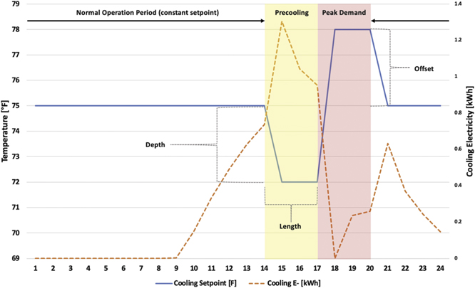
Figure 3. A sample thermostat setpoint schedule illustrating the simulation periods defined in table 1, with corresponding hourly electricity usage dedicated to air conditioning. For this schedule, the length of the precool is 3 h, the depth is 3 °F, and the offset is 3 °F. The AC setpoint (blue line) is lower than the baseline temperature in the middle of the day and higher than the baseline temperature during the peak demand period. The corresponding hourly AC electricity consumption (orange line) peaks in the middle of the afternoon (coinciding hours that have a relatively low average emissions factor, as shown in figure 1), and is lower during the evening hours (when the average emissions factor is relatively high during the diurnal period).
Download figure:
Standard image High-resolution image2.3. Thermal comfort
Thermal comfort was quantified according to predicted mean vote (PMV), as defined by the American Society of Heating, Refrigerating, and Air-Conditioning Engineers (ASHRAE). PMV is a non-linear function of dry bulb temperature, mean radiant temperature, air speed, relative humidity, metabolic rate, and clothing insulation, and describes the relative comfort of building occupants. A PMV of +0.5 (or −0.5) corresponds to a prediction that 10% of occupants will report themselves as uncomfortable (note that at a PMV of 0.0, 5% of occupants are still expected to report themselves as uncomfortable) [51]. Calculations of PMV were done in Python with the pythermal comfort model [52], with the variables air speed, metabolic rate, and clothing insulation held at constant values (0.1 m s−1, 1.2, and 0.5 respectively), and other measured hourly inputs provided by the EnergyPlus simulation. We used ASHRAE's defined comfort range of PMV values, which span −0.5 to +0.5 [51]. (Note: the AC setpoint in the baseline simulation was selected to give occupants a close to neutral thermal comfort level during afternoon and evening hours, with the best integer value found to be 75 °F.)
All 504 precooling schedules were simulated and any schedules that created uncomfortable conditions (per the PMV indicator) during the 5 to 8 pm peak demand period on any day in the simulation period were removed, leaving 70 distinct schedules that met the comfort conditions. While maintaining a PMV between −0.5 and 0.5 during the peak demand period was set as a criterion for the inclusion of a specific precooling schedule, PMV was allowed to go below this range during the pre-cooling period. Comfortable conditions were generally maintained throughout the entire day for shallow precooling schedules, but deep precools created uncomfortable conditions for occupants before 5 pm during the precooling period. We assume that occupants are either out of their home prior to this peak demand period or, as active participants in precooling, can adjust accordingly (e.g., wearing warmer clothes). Thermal comfort is also not considered overnight. (While the normal operation AC setpoint should ensure that occupants are not too warm, occupant comfort could also be affected by the natural gas heating setpoint, which is beyond the scope of this study.)
2.4. Output analysis
The key EnergyPlus output analyzed was hourly AC electricity consumption, which was used to quantify changes in peak demand period electricity consumption, total daily electricity consumption, and residential electricity cost. Hourly AC electricity consumption was also multiplied by average hourly CO2 average emissions factors for the CAISO grid to determine hourly CO2 emissions. Hourly emissions factors were calculated with grid level electricity load and emissions data (including both electricity imports and exports) from CAISO in 2019 [4] using the linear regression model described in equation (1). The model first bins hourly electricity load by month and hour of the day (ex. the bin 'June, hour 1', has 30 data points) and then regresses the hourly total CO2 emissions (E, in kg of CO2) on hourly total electricity load (D, in MWh) within each bin. The resulting coefficient D is defined as the average CO2 emissions factor (AEF, in kgCO2/MWh); a total of 288 coefficients were calculated with each coefficient representing a specific month and hour of the day.

Here, the subscripts h and m refer to the hour of the day and month of the year respectively, since the average emissions factor varies throughout the day due to changes in the grid mix. More information about the regression model can be found in the SI.
The hourly electricity consumption across all precooling schedules was analyzed from a residential electricity cost perspective assuming a time-of-use residential rate plan designed to reduce peak demand period consumption and offered by SCE, a utility within CAISO, servicing about 15 million people in Southern and Central California [34]. The SCE rate scheme applied for this analysis has a basic structure $0.52 per kWh from 5 to 8 pm, and $0.26 per kWh at all other times [53]. Total homeowner costs were calculated by multiplying the hourly electricity consumption by cost of electricity at that time.
3. Results
Relative to a constant setpoint scenario, precooling scenarios shift the timing and magnitude of both electricity consumption and the CO2 emissions associated with that electricity consumption. These scenarios also change electricity costs to the consumer. Post-filtering, the 70 remaining precooling schedules were evaluated relative to the baseline simulation by examining changes in electricity consumption, CO2 emissions, and residential electricity costs at the hourly level as well as cumulatively across the five month period.
3.1. Understanding the hourly impact of precooling
Using the simulation outputs for the month of September, we calculate hourly changes in electricity consumption, CO2 emissions, and residential electricity cost in order to analyze results at sub-daily timescales. (We highlight the month of September due to its high temperatures in the selected climate zone, which provided good conditions for understanding the potential impact of precooling on days when AC loads tend to be highest.) The measured hourly electricity consumption associated with each precooling schedule (or baseline schedule) was averaged for each hour of the day across the 31 days of September to create an average or representative September day for each unique schedule. This consumption was then used to determine the homeowner's associated electric utility costs and CO2 emissions. We then calculate the difference between a precooling schedule and the baseline schedule to get insight as to thermal behavior of the house over the course of the day and the resulting benefits and consequences.
The shallow and deeper precooling scenarios illustrated in figure 4 both shift peak demand period electricity consumption to other hours of the day, first increasing consumption during the precooling period, then reducing consumption during the peak demand period, and then again increasing consumption after the peak demand period. During the precooling period, the lower temperature setpoint causes an increase in AC output and a resulting increase in electricity consumption, with a larger increase the deeper the precool. During the peak demand period, when offset is occurring, the higher temperature setpoint reduces AC output and thus decreases electricity consumption. Deeper and longer precools will reduce AC consumption more during the peak demand period for a specific level of offset, but progressive increases in precooling depth or length offer progressively less reduction. In other words, there are diminishing returns for precooling when the goal is reduced peak period electricity consumption. After the peak demand period, returning the house to the baseline temperature causes a spike in electricity consumption as the AC turns on to reduce the indoor temperature back to the baseline setpoint. This increase could be mitigated by improving natural airflow, such as by opening windows, on nights when the outdoor temperature is below the post-8 pm setpoint of 75 °F. However, this study focuses solely on air-conditioning operation, and maintains the same window positions throughout the day for both the baseline cooling schedule and the precooling schedules. The magnitude of this spike is commensurate with the magnitude of the offset temperature reached at the end of the peak demand period (i.e., a 3 °F offset requires the AC to reduce the temperature by 3 °F starting at the end of the peak demand period).

Figure 4. Top: the changes in average hourly electricity consumption for a shallow precool (4 h length, 1 °F depth, 3 °F offset) scenario, as compared to the 75 °F baseline simulation, are shown in blue for an average day in the month of September. Bottom: the same is shown for a deeper precool (3 h length, 3 °F depth, 3 °F offset). Hourly PMV is shown in green, which stays between the +0.5 and −0.5 limits for both schedules.
Download figure:
Standard image High-resolution imageRegarding thermal comfort, occupants might experience a slightly cool sensation during precooling as the indoor air temperature is below the neutral-sensation temperature. For shallower precools, this sensation remains in the comfortable range, with PMVs above ASHRAE's lower bound of −0.5. However, deeper precools (3 °F or more) create indoor air temperatures significantly below the baseline temperature of 75 °F during the precooling, leading to PMVs below −0.5. Many of these deeper precools also created uncomfortable conditions during the peak demand period, and thus were eliminated in the PMV filtering stage, but a small number of precools with a depth of 3 °F created uncomfortable conditions during the precooling period but not during the peak demand period, and thus are included in this analysis. During the peak demand period, occupants would experience a slightly warm sensation due to the elevated indoor temperature that is proportional on the amount of offset, but all schedules included in these results maintain PMV levels between 0 and +0.5, the maximum permitted level. After the peak demand period, the PMV level approaches 0, or a neutral sensation, as the house returns to the baseline temperature.
These precooling scenarios shift the magnitude and timing of when CO2 emissions (figure 5) and residential electricity costs (figure 6) occur by moving them from the peak demand period to normal operation hours, following the same general temporal trends as changes in electricity consumption. These changes are scaled by the hourly AEFs for CO2 emissions, and by the hourly price of a kWh of electricity for residential electricity costs. For example, the large difference between peak demand period electricity price and off period electricity price (factor of 2x) creates larger reductions (relative to the baseline) in residential electricity cost during the peak demand period than increases in cost during the precooling period. It is important to note that the AEFs and the price structure serve as hourly multipliers, making it possible for reductions in cumulative CO2 emissions or residential electricity costs, even if total electricity consumption is unchanged or even increased. With a better understanding of the hourly impacts of precooling, we move next to an analysis of the aggregate results over a cooling season.

Figure 5. Top: the changes in average hourly CO2 emissions between a shallow precool (4 h length, 1 °F depth) and the 75 °F baseline simulation are shown in blue for the month of September. Bottom: the same is shown for a deeper precool (3 h length, 3 °F depth). Hourly PMV is shown in green.
Download figure:
Standard image High-resolution image
Figure 6. Top: the change in average hourly residential electricity costs for a household for a shallow precool (4 h length, 1 °F depth) compared to the 75 °F baseline simulation is shown in blue for the month of September. Bottom: the same is shown for a deeper precool (3 h length, 3 °F depth). Hourly PMV is shown in green.
Download figure:
Standard image High-resolution image3.2. Cumulative impact of precooling
The precooling schedules were also analyzed over the entire five-month period from May through October by summing the hourly outputs for each hour in this period to get aggregate results for the AC electricity consumption, CO2 emissions, and residential electricity cost, respectively.
The data points lying below the dashed horizontal axis of figure 7 represent precooling strategies that are effective in simultaneously reducing CO2 emissions, peak demand period electricity consumption, and residential electricity costs. While all the precooling schedules simulated reduce peak demand period electricity consumption, the schedules that achieved the most reduction feature large amounts of offset, deep precools, and, to a lesser extent, long precools. Increasing the depth of the precool or the amount of offset increases the gap between the initial temperature of the house during the peak demand period and the temperature at which the AC cycles back on. This leads to a longer period during which the AC is inactive as the house warms from the precooling period temperature to the offset period temperature. Increasing the length of the precool reduces peak demand period consumption due to the increased removal of heat from portions of the building that contribute to thermal mass beyond the air itself. In other words, the longer the precool, the more heat is removed from the internal walls and furniture, thus slowing the rate of indoor air temperature increase when the precooling period ends. However, increasing in the length of a precool provides a much smaller reduction in peak demand period consumption than increasing the depth of the precool or the amount of offset. In summary, schedules with deep precools and large offsets create conditions in which the AC operates for only a small portion of the peak demand period, effectively reducing peak demand period consumption, and this reduction in AC operation can be reduced slightly more with longer precools that help to keep the house cool during the peak demand period. The precools that reduce peak demand period consumption the most achieve a reduction of around 70%.

Figure 7. Each dot represents one of the 70 distinct precooling schedules that passed the PMV comfort test. The x-axis shows percent change in aggregate peak demand period consumption and the y-axis shows the percent change in CO2 emissions between the cooling schedule and the baseline simulation over the five-month period. The color of each dot represents the percent change in residential electricity cost over this same period. Cooling schedules are illustrated by the black bars and groupings, with the width of the bar proportional to the length of the precool, the height of the bar proportional to the depth of the precool, and the offset shown by each grouping.
Download figure:
Standard image High-resolution imageOver half of the simulated schedules increase CO2 emissions, but some schedules achieve small reductions in emissions relative to the baseline. Schedules that reduce CO2 emissions generally feature 2 °F or less of depth, with the most effective schedules being those that have large amounts of offset, and only 1 °F of depth. Precools deeper than 1 °F often have the effect of increasing total electricity consumption, despite decreasing peak demand period consumption. CO2 emissions reductions are possible for these schedules that increase total electricity consumption since consumption is shifted from the peak demand period, when there are higher AEFs, to the precooling period, when there are lower AEFs, but these results suggest that for most deeper precools, the increase in electricity consumption is significant enough that the difference between precooling period AEFs and peak demand period AEFs cannot compensate. Instead, the shallow precooling schedules that are most effective in reducing emissions feature a large offset that reduces the peak demand period consumption when AEFs are high but do not significantly increase total electricity consumption. The most effective schedules at decreasing CO2 emissions achieve reductions of approximately 3%–3.5%.
The schedules that achieve residential cost savings tend to overlap with the schedules that accomplish significant CO2 emissions reductions. A higher fraction of precooling schedules reduce residential electricity costs than reduce emissions because of the large difference between the on- and off-peak pricing (factor of 2x) schedule considered in this analysis. This makes it possible for a precooling schedule to significantly reduce residential costs despite increasing total electricity consumption. This result implies that deeper precools would need precooling period emissions factors to be less than 50% of peak demand period emissions factors in order for deeper precools to successfully reduce emissions, which is not the case for the AEFs used in this study. The effect of this large price multiplier is also seen in the magnitude of cost reductions, with the optimal precooling schedule reducing residential electricity bills by nearly 13%, outpacing the CO2 emissions reductions.
The precooling schedules that simultaneously reduced peak demand period consumption, CO2 emissions, and residential cost feature large offsets of 2 to 3 °F, and, in general, use shallower precools of varying length; the most successful schedules feature 1 °F of precooling for 1–5 h. This type of schedule has enough offset to significantly reduce peak demand period consumption but does not feature the deep precools that significantly increase total electricity consumption and make reductions in CO2 emissions impossible. Figure 8 shows the subset of 3 °F offset schedules from figure 7, with the schedule that reduced peak period electricity consumption most and the schedule that simultaneously reduced both cost and CO2 emissions most highlighted in purple and orange, respectively. The ten schedules that most reduced CO2 emissions are included in the table below, with full results of all the schedules included in the SI.

Figure 8. Includes subset of 3 °F offset scenarios from figure 7. The schedule that reduced peak period cooling electricity most is shown with purple bars, and the schedule that reduced peak period cooling electricity consumption and CO2 emissions most is shown with orange bars. The color scale for residential cost is maintained from figure 7.
Download figure:
Standard image High-resolution image
Table 2, row 7, shows that a significant amount of CO2 and cost reductions can be achieved with the use of an offset in the absence of any precooling (i.e. constant setpoint of 75 °F in all hours before the peak demand period) due to the reduced AC operation during the peak demand period. Introducing a shallow precooling schedule, in combination with this offset, significantly increases the reduction in peak demand period electricity consumption, and the presence of the hourly AEFs and cost profile make it possible for this to simultaneously provide slightly bigger reductions in both CO2 emissions and cost. Therefore, under the selected SCE utility pricing schedule and with emissions calculated using hourly AEFs, shallow-precools outperform the strategy of simply using a higher AC setpoint during peak demand period hours.
Table 2. The ten schedules most effective at reducing CO2 emissions and the associated changes in CO2 emissions, cost, and peak demand period consumption.
| Offset | PC | PC | Change in peak demand period | Change in residential cost (%) | Change in CO2 emissions (%) |
|---|---|---|---|---|---|
| hours | depth | electricity consumption (%) | |||
| 3 | 2 | 1 | −57 | −13 | −3.5 |
| 3 | 1 | 1 | −55 | −12 | −3.0 |
| 3 | 4 | 1 | −57 | −12 | −2.9 |
| 3 | 5 | 1 | −58 | −12 | −2.6 |
| 3 | 3 | 1 | −57 | −12 | −2.5 |
| 2 | 2 | 1 | −42 | −9.0 | −2.5 |
| 2 | 0 | 0 | −33 | −8.1 | −2.5 |
| 3 | 6 | 1 | −58 | −11 | −2.3 |
| 2 | 1 | 1 | −40 | −8.5 | −2.0 |
| 3 | 1 | 2 | −61 | −12 | −2.0 |
4. Discussion
Several simplifications or assumptions were necessary to complete the modeling phase of this study. For example, the building prototype used for this model, though well vetted by PNNL to represent an average building at the national level, may not be as representative of homes in California, and in Southern California specifically, even with the most common foundation and heating/cooling technology selected. California homes are smaller than the prototype used here on average.
This simulation assumes active AC setpoints for all hours of the day. In reality, residents who are not home in the middle of the day may turn off their ACs entirely while out of the house. This study does not attempt to compare precooling results to other intermittent AC usage schedules, only to a constant setpoint schedule. Some deep precooling schedules also reduced indoor temperatures below the comfortable range during the precooling period, which limits the time that occupant comfort can be ensured. Residents would need to either accept this risk of discomfort and adapt accordingly (e.g., with warmer clothing), or be absent during the precooling period. In reality, individuals will have unique tolerances for feeling 'too warm' versus 'too cold'; the PMV metric used here only expresses average population-level comfort preferences. While the specific implementation of precooling is beyond the scope of this paper, the increasing penetration of smart homes, appliances, and thermostats could make precooling easier for homeowners via preset thermostat schedules.
Lastly, this study relied on hourly average emissions factors for the CAISO. Average emissions factors represent the current mix of sources supplying power to the grid in a time period, but a more accurate estimation of the emissions associated with shifting the timing of electricity consumption may come from the use of marginal emissions factors. In this case, CO2 emissions would be calculated by multiplying the hourly change in electricity consumption with hourly marginal emissions factors. While there is not currently an established set of marginal emissions factors for CAISO, these factors could be estimated with a model similar to the regression model used in this study, but instead of regressing total hourly CO2 emissions on total hourly changes in demand, one would regress changes in hourly CO2 emissions on changes in hourly demand. Using marginal, instead of average, emissions factors may increase the amount of calculated CO2 emissions reductions, potentially making deeper precools more beneficial, as marginal emissions factors are particularly high during the grid ramping that occurs in early evening since natural gas combustion generators are typically at the margin [54].
5. Conclusion
This study used EnergyPlus to evaluate the efficacy of residential precooling as a strategy to reduce CO2 emissions in grids that have periods of high variable renewable energy penetrations in addition to providing the demand response and load-levelling benefits that are traditionally associated with precooling. Our results suggest that in CAISO, precooling can achieve multi-faceted benefits in terms of flattening CAISO's net demand curve as well as reducing CO2 emissions, residential utility costs, and peak demand electricity usage, even at the expense of an overall increase in total residential electricity use. Relative to a constant AC setpoint, simultaneous reductions of 57% of peak demand period consumption, 3.5% of CO2 emissions, and 13% of residential cost is possible to achieve when precooling a typical home in California CZ9 over the five-month period studied in this analysis.
Key insights from this study include:
- CO2 emissions benefits were realized in many precooling schedules despite increases in total electricity demand due to the daytime decoupling between electricity consumption and greenhouse gas emissions within CAISO, a grid with high penetrations of daytime variable renewable energy resources.
- Achieving larger reductions in peak demand period electricity consumption typically required larger total electricity consumption penalties.
- While deep precools reduced peak demand period consumption more than shallow precooling schedules, they often caused an increase in total CO2 emissions due to large increases in total electricity demand.
- Shallow precools could significantly reduce peak demand period consumption while also decreasing total CO2 emissions due to more mild increases in total electricity consumption than deep precools.
- Residential precooling strategies can also provide economic benefits to the consumers when utility rate structures use higher costs to penalize electricity usage during peak hours
The results of this study confirm that the timing of electricity consumption (as opposed to simply the magnitude of electricity consumption) is becoming increasingly important as grids transition to higher penetrations of variable renewable power sources, and can inform the implementation of precooling as a demand response strategy within CAISO. For example, shallow precools of 1–2 °F below the baseline temperature with precooling periods of 1 to 4 h in length can achieve demand response benefits without increasing total CO2 emissions or causing large periods of discomfort. Thus, the real-time variations in grid mix create an opportunity for optimizing precooling as an emissions reduction strategy. This conclusion offers important policy insights, particularly for grids that have high penetrations of daytime variable renewable energy resources. Given the pace of energy transitions around the world, we believe that this study is a significant contribution to the literature for researchers, industry members, and policy makers interested in designing strategies that meet climate mitigation and demand response priorities simultaneously.
Whereas our goal was to evaluate multifaceted tradeoffs of precooling for peak electricity demand, the environment, and occupants, future studies could design precooling schedules that have the explicit goal of minimizing cooling-associated CO2 emissions. Minimizing emissions may involve changing the timing of the precooling period, which currently occurs directly before the peak demand period and partially overlaps with the rapid ramping of net demand that occurs in the late afternoon (see figure 1). Implementing precooling prior to this ramping period, instead of overlapping with it, may offer larger reductions in CO2 emissions due to the rapid increases in average and marginal emissions factors that occur during the ramping period due to the rapid deployment of fast-reacting natural gas generators needed to meet rising demand as solar resources diminish.
Data availability statement
The data that support the findings of this study are available upon reasonable request from the authors.
Footnotes
- *
The funding sources that supported this work include: NSF Award Id: 1845931; title: CAREER: coordinating climate change mitigation and adaptation strategies across the energy-water nexus: an integrated research and education framework.