Leveraging trust for joint multi-objective and multi-fidelity optimization

Acquisition functions encompass a broad class of functions that can be constructed using the posterior distribution of the GP model. The effectiveness of an acquisition function is assessed based on its ability to converge to the global optimum, with minimal evaluations of the objective function. This can be best illustrated through a series of diagrams shown in figure 1, depicting the iterations of Bayesian optimization loop starting from three initial points. After constructing a GP model with a mean (solid blue line) and variance (shaded region), an acquisition function is derived (bottom plot). This acquisition function is then optimized, often using gradient methods, to identify its maximum, which corresponds to the next evaluation point for the black-box objective function. The choice of the acquisition function significantly impacts the convergence of Bayesian optimization towards the global optimum. This section provides an overview of some widely recognized acquisition function policies discussed in the existing literature. We would like to note that the development of acquisition functions is still an active area of research, with some recent contributions using for instance distance correlation [20] or deep neural networks [21].

Zoom In Zoom Out Reset image size

Assuming that the objective function has been evaluated n times generating a data set $D_{n} = \{({\boldsymbol{x}}_{1},y_{1}),$ $({\boldsymbol{x}}_{2},y_{2}),{\ldots},({\boldsymbol{x}}_{n},y_{n})\}$, these acquisition functions propose the optimal choice for the subsequent evaluation point, denoted as ${\boldsymbol{x}}_{n+1}$. Please note that x is a vector of input parameters while the function output y is a single scalar value for this section. This selection is achieved through the optimization of a derived metric, taking into account the information from previously evaluated points. Specifically, the next evaluation point is given by ${\boldsymbol{x}}_{n+1} = \arg\max_{{\boldsymbol{x}}\in\mathcal{X}}A({\boldsymbol{x}}|D_{n})$, where $\mathcal{X}$ is the input parameter domain and $A({\boldsymbol{x}}|D_{n})$ represents one of the acquisition functions given the dataset D_n detailed below.

One widely used acquisition function is the upper confidence bound (UCB) policy [22], which is alternatively referred to as the lower confidence bound for minimization tasks. The UCB acquisition function is expressed as:

$$\begin{equation} \text{UCB}\left({\boldsymbol{x}}|D_{n}\right) = \mu_{n}\left({\boldsymbol{x}}\right) + \kappa\sigma_{n}\left({\boldsymbol{x}}\right), \end{equation} \tag{ 1 }$$

where $\mu_{n}({\boldsymbol{x}})$ and $\sigma_{n}({\boldsymbol{x}})$ denote the mean and the standard deviation of the function value under the posterior distribution $p(y|{\boldsymbol{x}},D_n)$, respectively, derived from GPs. The hyperparameter κ is used to balance exploration and exploitation. UCB is popular due to its simplicity and effectiveness in practice.

Another well-known acquisition function in Bayesian optimization is expected improvement (EI) [23], which suggests the next evaluation point based on the EI over the current optimal objective value $y^*$. The EI acquisition function is expressed as:

$$\begin{equation} \text{EI}\left({\boldsymbol{x}}|D_{n}\right) = \mathbb{E}\left[\max\left(f_{n+1}\left({\boldsymbol{x}}\right) - y^*, 0\right)\right], \end{equation} \tag{ 2 }$$

where, $\max(f_{n+1}({\boldsymbol{x}})$ is drawn from the posterior distribution and $\mathbb{E}$ denotes the expectation symbol, representing an average over the probability distribution defined by the Gaussian process (GP) model. A variation of EI is the knowledge gradient (KG) acquisition function [23, 24], which relies entirely on the posterior model. KG selects the next evaluation point based not on the best observable value but on the best value of the posterior mean. The KG acquisition function is given by:

$$\begin{equation} \text{KG}\left({\boldsymbol{x}}|D_{n}\right) = \mathbb{E}\left[\max_{{\boldsymbol{x}}^{^{\prime}} \in \mathcal{X}}\left(\mu_{n+1}\left({\boldsymbol{x}}^{^{\prime}}\right)\right)\right] - \max_{{\boldsymbol{x}}^{^{\prime}} \in \mathcal{X}}\left(\mu_n\left({\boldsymbol{x}}^{^{\prime}}\right)\right), \end{equation} \tag{ 3 }$$

where the terms $\mu_{n+1}({\boldsymbol{x}})$ and $\mu_n({\boldsymbol{x}})$ represent the posterior mean of the GP after n + 1 and n evaluations, respectively. The term $\mu_{n+1}({\boldsymbol{x}})$ represents the posterior mean of the GP after including an additional data point $({\boldsymbol{x}}, f({\boldsymbol{x}}))$, where $f({\boldsymbol{x}})$ is the realization of the stochastic process at location x . This captures the updated belief about the function based on the new data point. The term $\mu_n({\boldsymbol{x}})$ represents the prior belief before the new data point is included. KG is more exploratory than EI as it is influenced by posterior changes throughout the domain.

Information-theoretic acquisition functions utilize the mutual information $I({\boldsymbol{x}};{\boldsymbol{x}}^*)$ between a specific location in the parameter domain and the observed data set. One such function is Entropy Search (ES) [25], represented mathematically as:

$$\begin{equation} \text{ES}\left({\boldsymbol{x}}|D_{n}\right) = H\left(p\left({\boldsymbol{x}}^*|D_{n}\right)\right) - \mathbb{E}\left(H\left(p\left({\boldsymbol{x}}^*|D_{n},{\boldsymbol{x}},f\left({\boldsymbol{x}}\right)\right)\right)\right), \end{equation} \tag{ 4 }$$

where H denotes Shannon's entropy and $p({\boldsymbol{x}}^*|D_{n})$ refers to the probability distribution for the position of the maximum given currently observed data. Moreover, $p({\boldsymbol{x}}^*|D_{n},{\boldsymbol{x}},f({\boldsymbol{x}}))$ is the probability distribution for the position of the maximum given data D_n as well as x and $f({\boldsymbol{x}})$, where $f({\boldsymbol{x}})$ is drawn from the GP trained on D_n . The left term in the equation represents the entropy of the posterior distribution of the maximizing location ${\boldsymbol{x}}^*$, while the right term depicts an expectation over the entropy of the posterior after an additional sample. In higher-dimensional input spaces, evaluating the mutual information between the point to be queried and the maximizing location ${\boldsymbol{x}}^*$ becomes challenging. To address this, computationally more efficient variations have been introduced. MES [26] utilizes the mutual information between the maximum value $y^*$ rather than ${\boldsymbol{x}}^*$. The MES acquisition function is formulated as:

$$\begin{equation} \begin{aligned} \text{MES}\left({\boldsymbol{x}}|D_{n}\right) = H\left(p\left({\boldsymbol{y}}^*|D_{n}\right)\right) - \mathbb{E}\left(H\left(p\left({\boldsymbol{y}}^*|D_{n},{\boldsymbol{x}},f\left({\boldsymbol{x}}\right)\right)\right)\right). \end{aligned} \end{equation} \tag{ 5 }$$

MES offers comparable or even better performance than ES while being significantly faster to compute [26]. It should be noted that MES may perform sub-optimally in certain conditions since it assumes noiseless observations only [27].

As we outlined in the introduction, there exist many use cases in which the objective consists of multiple sub-goals. One can think of these sub-goals as a vector of solutions, which has to be reduced to a scalar number to be compatible with conventional numerical optimization schemes. This reduction, or scalarization, is often not straightforward and the weights given to each sub-goal are usually found empirically. A potent strategy for such use cases is MO optimization, where one tries to increase the diversity of solutions. In this case, the function that is being maximized can be expressed as a vector of functions

$$\begin{align*} {\boldsymbol{f}}\left({\boldsymbol{x}}\right) = \begin{pmatrix}{f^{\,{\left(1\right)}}\left({{\boldsymbol{x}}}\right)} \\f^{\,{\left(2\right)}}\left({\boldsymbol{x}}\right) \\ \dots \end{pmatrix} \end{align*}$$

that are evaluated to yield output vectors

$$\begin{equation*} {\boldsymbol{y}}\left({\boldsymbol{x}}\right) = \begin{pmatrix}{y^{\left(1\right)}\left({{\boldsymbol{x}}}\right)} \\y^{\left(2\right)}\left({\boldsymbol{x}}\right) \\ \dots \end{pmatrix}. \end{equation*}$$

The optimum solution in this case consists of a solution vector. A useful concept describing this situation of not just a single optimum but a set of optimal points in the multi-dimensional objective space is the Pareto efficiency [11], which is visualized as the Pareto front ($\mathcal{P}$). To describe the Pareto front, the notion of domination is outlined in definition 1. The Pareto front is composed of a set of non-dominated points in the output space as shown in figure 2.

Zoom In Zoom Out Reset image size

One of the simplest algorithms for MO optimization is Pareto Efficient Global Optimization (ParEGO) proposed by Knowles [30]. ParEGO is a scalarization-based approach in which a single-objective optimizer is employed to find the Pareto front. In this algorithm, scalarization is achieved using a weighted sum of the objective functions with random weights generated at each iteration. The main advantage of ParEGO over other scalarization methods is that the random weights allow for exploring the Pareto front for a diverse set of solutions without predefining the weights or relying on user preferences. By iteratively running this algorithm with new weights, it becomes possible to approximate the entire Pareto optimal set.

Alternatively, one can reframe the MO problem as a single-objective optimization by using a new objective that implicitly increases solution diversity. One such criterion is the Hypervolume (HV) Indicator. HV is defined as the n-dimensional volume of the output subspace covered from a reference point, always taken to be zero in this work, to a set of points in the objective space. Using this definition of HV, we can then proceed to define Hypervolume Improvement (HVI) as

$$\begin{equation} \mbox{HVI} \left(\mathcal{P},{\boldsymbol{y}}\right) = \mbox{HV}\left(\mathcal{P} \cup {{\boldsymbol{y}}}\right) - \mbox{HV} \left(\mathcal{P}\right). \end{equation} \tag{ 6 }$$

Equation (6) describes the difference between the current HV and one with an additional output point y [31]. If the set of points making up $\mathcal{P}$ already dominate y then $\mathrm{HVI} = 0$, because there is no HV gained by adding the point y .

HVI can be used to generalize the EI policy described in section 1.2 to the MO scenario. First proposed by Emmerich et al [32], this method is called Expected Hypervolume Improvement (EHVI). Following the definition from Yang et al [31], we can write this as

$$\begin{equation} \mbox{EHVI}\left({\boldsymbol{x}}|D_n\right) = \mathbb{E}\left(\mbox{HVI}\left(\mathcal{P},{\boldsymbol{y}}\right)\right) = \int \mbox{HVI}\left(\mathcal{P},{\boldsymbol{y}}\right)\; p\left({\boldsymbol{y}}|{\boldsymbol{x}}, D_n\right) \,\mathrm{d}y. \end{equation} \tag{ 7 }$$

This infill criterion has been demonstrated to achieve a good convergence to the true Pareto front [33–35].

A common criticism of the EHVI acquisition function has been the time complexity involved in calculating it. A first closed-form calculation of EHVI was implemented by Emmerich et al [36] with a computational complexity $\mathcal{O}(n^3\log{}n)$ for a 2D output space. Over the years with efforts by Hupkens et al [37], Emmerich et al [38] and Yang et al [39] the time complexity for 2D and 3D case has been reduced to $\mathcal{O}(n\log{}n)$. In this work an implementation of EHVI available on BoTorch based on estimating gradients using auto-differentiation is used as described by Daulton et al [40]. This exploits the high number of cores that are available with modern GPUs to make EHVI optimization fast and applicable to real-world scenarios. While we have focused our discussion on EHVI, it should noted that information theoretic acquisition functions such as entropy search can also be adapted to MO scenarios [41, 42].

In many real-world optimization problems, multiple information sources with varying degrees of fidelity are available. These sources can provide different levels of accuracy, typically with a trade-off between data fidelity and cost. Integrating such MF data into single-objective optimization algorithms is an essential way to improve the optimization process [14, 43–47].

Let us denote the input search parameters as ${\boldsymbol{x}}\in \mathcal{X}$ and the fidelity parameters as ${\boldsymbol{s}}\in \mathcal{S}$ where $\mathcal{X}$ and $\mathcal{S}$ are the input and fidelity spaces respectively. Importantly, in our GP model, fidelity s is treated as a regular input dimension alongside x . This means that fidelity s is accounted for in the kernel of the GP, allowing us to make probabilistic inferences conditioned on both x and s . For more details on the choice of GP kernels, the reader is referred to appendix. The goal is to build a surrogate model that incorporates information from ${f({\boldsymbol{x}},{\boldsymbol{s}})}$. The challenge in MF optimization is to effectively balance the trade-off between information and cost while ultimately finding a global maximum at the target fidelity. This target fidelity usually corresponds to the highest fidelity which is also the most expensive information source.

One intuitive solution to this problem is the two-step approach proposed by Lam et al [48]. In this approach, the selection of the next point to probe in x is done separately from the fidelity choice s . To achieve this, Lam et al use an EI policy that is evaluated at the target fidelity only. Lower fidelity measurements are implicitly incorporated into this process, as they affect the surrogate model at the highest fidelity. Once a suitable position has been identified in x , the ideal fidelity for probing this point is chosen by comparing the predicted reduction in uncertainty or gain in knowledge with the computational cost involved.

An alternative approach is to combine both the selection of the next point and the weighting by the expected knowledge gain per unit cost in a single step. Notably, MES and KG acquisition functions can be adapted with minor changes for this kind of MF optimization. For KG [49, 50], the acquisition function is conditioned on the best value of the posterior mean at the target fidelity ${\boldsymbol{s}}^*$ ($\max_{{\boldsymbol{x}}\in\mathcal{X}}(f({\boldsymbol{x}},{\boldsymbol{s}}^*))$) rather than the best value of the posterior mean. In the case of MES, the mutual information between the maximum value $y^*$ at the highest fidelity and the data set is maximized. This gain of information is then divided by the computational cost that is a function of fidelity s [51]. The resulting MF MES acquisition function is then given by a simple modification to equation (5):

$$\begin{equation} \mbox{MF$-$MES}\left({\boldsymbol{x}},{\boldsymbol{s}}|D_{n}\right) = \frac{\mbox{MES}\left({\boldsymbol{x}}|D_{n}\right)}{\mbox{cost}\left({\boldsymbol{s}}\right)}. \end{equation} \tag{ 8 }$$

Similar MF policies can be developed for other exploratory acquisition functions, such as the UCB [52, 53].

Our proposed optimization scheme hinges on the joint optimization of a function and our trust in the information source that yields the results. We use 'trust' to express our confidence level in the outcomes generated by the information source at various levels of fidelity. This formulation allows us to recast MF optimization as a MO problem, with trust $\theta({\boldsymbol{s}})$ and output objectives $f({\boldsymbol{x}})$ forming the two poles of optimization. Hence, we aim to optimize the following function output:

$$\begin{equation} {\boldsymbol{f}}\left( {\boldsymbol{x}},{\boldsymbol{s}}\right) = \begin{pmatrix}{{\boldsymbol{f}}\left({{\boldsymbol{x}}}\right)} \\ \theta\left({\boldsymbol{s}}\right) \end{pmatrix}. \end{equation} \tag{ 9 }$$

The trust objective $\theta({\boldsymbol{s}})$ is central to the proposed optimization scheme. High fidelity sources, usually more costly, are intrinsically more trustworthy than their low fidelity counterparts due to their higher accuracy and reliability, and thus, trust is a function that grows monotonically with fidelity. In the simplest case, one can assume that there is a constant increase in trust as the fidelity parameter is raised and correspondingly, the trust would be equal to the fidelity itself, $\theta(s) = s$. A more rigorous approach may involve an actual measure of trust, e.g. linking the notion of trust to concepts such as mutual information. In these scenarios, the trust objective can be seen as an approximation that reflects the average mutual information shared across fidelities. For numerous circumstances, like simulations where the outputs at increasing fidelity converge, an appropriate trust curve follows approximately $\theta(s) \approx \tanh(s)$. We discuss the influence of the trust objective on the optimizer in more detail in section 3.3.3.

As discussed in section 2.2, we can optimize a problem of the form equation 9. using, for instance, EHVI. This acquisition function strives to increase the joint HV encapsulated within the Pareto front of $f({\boldsymbol{x}}, {\boldsymbol{s}})$ and $\theta({\boldsymbol{s}})$. Due to the ascending nature of trust value, the optimizer is predisposed to probe points with the highest trust. In a MF context where computational or experimental costs are not uniform, the acquisition function can be normalized by incorporating a cost penalty, specifically by dividing the value of the acquisition function by the corresponding cost (section 2.3). This adjustment to the acquisition function ensures that the optimization process selectively probes the point that maximizes the ratio of EHVI to the associated computational or experimental cost. As a result, the acquisition function optimizes our knowledge of the Pareto front and Pareto set on a per-unit-cost basis. The final acquisition function is then written as

$$\begin{equation} \mbox{Trust-MOMF}\left({\boldsymbol{x}},{\boldsymbol{s}}|D_{n}\right) = \frac{\mbox{EHVI}\left({\boldsymbol{x}},s|D_{n}\right)}{\mbox{cost}\left({\boldsymbol{s}}\right)}. \end{equation} \tag{ 10 }$$

where $\mathrm{EHVI}({\boldsymbol{x}},{\boldsymbol{s}})$ signifies that the complete objective comprises both the normal output objectives and the trust objective. The entire structure of this approach for Trust-MOMF optimization is outlined in algorithm 1.

Algorithm 1. Trust-based Multi-Objective Multi-Fidelity Optimization (Trust-MOMF).
Inputs:
$\bullet$ Probed dataset Dn
$\bullet$ Gaussian process models $GP_1,\ldots,GP_k$
$\bullet$ Fidelity function s , cost function $C({\boldsymbol{s}})$
$\bullet$ Total computational budget Ctotal
Outputs: Optimal Pareto front $\mathcal{P}^*$
1: Initialization:
Generate ninit initial data points Dn
Fit Gaussian process models $GP_1,\ldots,GP_k$
Initialize Pareto front $\mathcal{P} = \emptyset$
Initialize spent budget $C_{\text{spent}} = C_{\text{init}}$
2: While $C_{\text{spent}} \lt C_{\text{total}}$ do
3: Optimization step:
Optimize the Trust-MOMF acquisition function, equation (10)
$({\boldsymbol{x}}_{n+1},{\boldsymbol{s}}_{n+1}) \gets \arg\max_{{\boldsymbol{x}}, {\boldsymbol{s}}} \left[ \frac{\text{EHVI}({\boldsymbol{x}}, {\boldsymbol{s}})|D)}{C({\boldsymbol{s}})} \right]$
4: Probe problem at selected position and fidelity:
${\boldsymbol{y}}_{n+1} \gets \text{Problem}({\boldsymbol{x}}_{n+1}, {\boldsymbol{s}}_{n+1})$
5: Data and model updates:
Update dataset $D_{n+1} \gets D_{n} \cup \{({\boldsymbol{x}}_{n+1}, {\boldsymbol{s}}_{n+1}, {\boldsymbol{y}}_{n+1}) \}$
Re-fit Gaussian process models $GP_1,\ldots,GP_k$
Update Pareto front $\mathcal{P}$
Increment Cspent by $C({\boldsymbol{s}}_{n+1})$ and n by 1
6: Terminate

The algorithm starts with a random initialization of n points that result in a data set $D_{n} = \{({\boldsymbol{x}}_{1},{\boldsymbol{s}}_{1},{\boldsymbol{y}}_{1}),$ $({\boldsymbol{x}}_{2},{\boldsymbol{s}}_{2},{\boldsymbol{y}}_{2}),{\ldots},({\boldsymbol{x}}_{n},{\boldsymbol{s}}_{n},{\boldsymbol{y}}_{n})\}$. With this data set, k number of GP models are fitted corresponding to k output objectives. The initial cost C_init utilized until this point is the cost undertaken to generate the D_n . After the initialization, the acquisition function is optimized to yield both the new input and fidelity position where the problem is then probed. This generates a new data sample $({\boldsymbol{x}}_{n+1},{\boldsymbol{s}}_{n+1},{\boldsymbol{y}}_{n+1})$ that is used to update the data set and re-fit the GP models. The last step is to update the spent cost C_spent and check whether we exceeded our computational budget C_total. The process is terminated when the spent cost becomes greater or equal to our available computational budget.

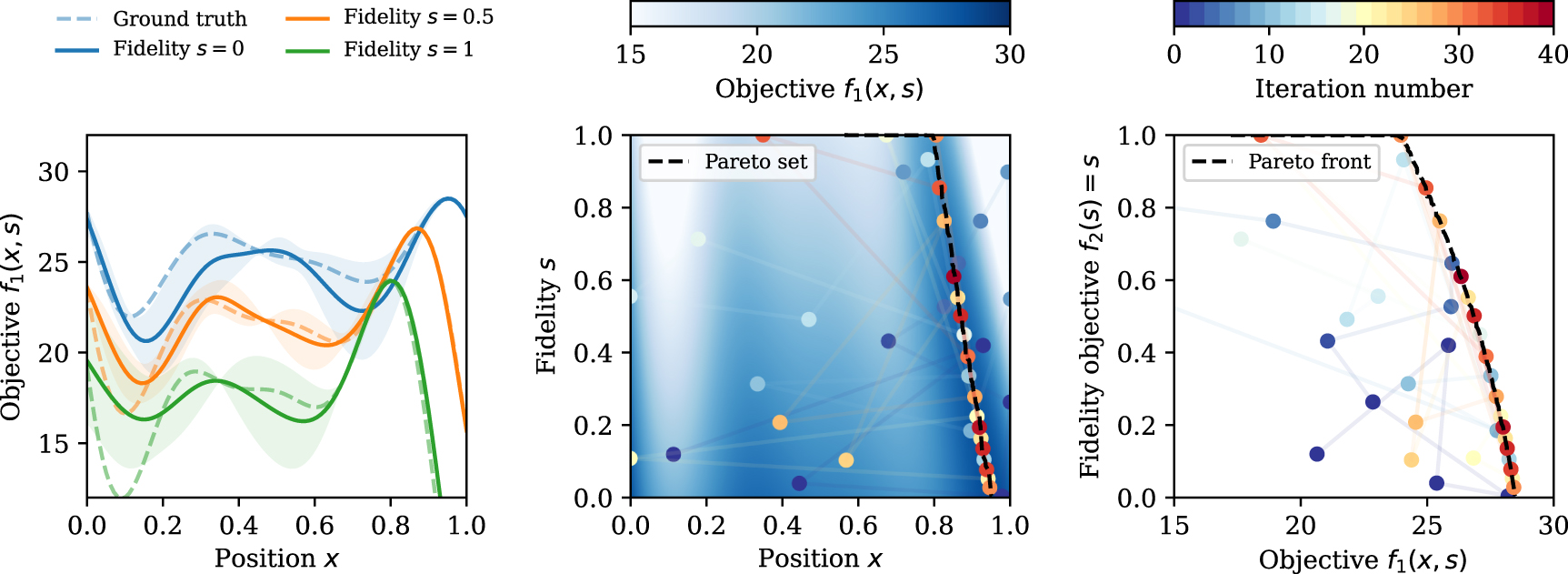
Figure 3 exemplifies the optimization of a 1D Forrester function by integrating information from lower fidelity data that incur reduced cost. In this test case, trust is assumed linear ($\theta(s) = s$) and the cost is modeled as $C(s) = \exp [a\cdot s]$, with a = 5, rendering an evaluation at maximum fidelity (s = 1) approximately 150 times costlier than at minimum fidelity (s = 0). This cost function can be substituted with any other monotonically increasing function. A key assumption of the Trust-MOMF method is that the Pareto set, which underlies the Pareto front, belongs to a similar region in the search space, thereby facilitating efficient translation of information across fidelities. It is important to note that this method, akin to all MF approaches that leverage knowledge transfer, becomes less efficient if the Pareto set experiences significant shifts between fidelities.

Zoom In Zoom Out Reset image size

Finally, we would like to point out that this method can be expanded to include multiple fidelity dimensions $s^{(m)}$ where m represents the number of fidelity dimensions. This is especially useful for multi-dimensional numerical models with individual resolution parameters for each dimension. Depending on the problem, these individual fidelity dimensions can either be managed via a single, unified trust objective or treated as separate dimensions within the optimization problem. However, it should be noted that the EHVI algorithm does not scale efficiently to many output dimensions, and the sequential MOMF method introduced in the next section may be a more suitable alternative when numerous fidelity dimensions need to be optimized individually. The different fidelity dimensions can also be discrete or categorical in nature where they take on finite values. The trust-MOMF method still applies but the optimization of the acquisition functions needs to be adapted. One example is mixed acquisition function optimization as performed in botorch for input spaces that include both continuous and discrete input parameters.

While we have so far discussed the benefits and implementation of joint Trust-MOMF optimization, an alternative approach worth exploring is a sequential version of the MOMF optimization. This sequential optimization scheme, inspired by the work of Lam et al [48] on single-objective optimization, separates the selection of the next position to probe and the fidelity choice into two distinct steps, thus bringing a different perspective to MF optimization. In the following, we will present and discuss this method, outlining its main principles, operational procedures, and potential benefits. This sequential MOMF approach will also serve as a benchmark to evaluate the extent to which our problems benefit from a joint optimization strategy.

In this scheme, the first step after initialization is to get a candidate position in the input space ${\boldsymbol{x}}_{n+1}$. This position selection step is identical to conventional MO optimization, see section 2.2. In algorithm 2 and the subsequent examples, we use EHVI for this task. Once the candidate point is identified, we can move on to fidelity selection. For this step, the GP first needs to be scalarized at this particular position. Here this is done by summing all the objectives with equal weights. This is done to avoid any preference between objectives and is motivated by the fact that all the objective functions change at a similar scale (due to a normalization step in the data processing that scales outputs of all objectives to the range $[0,1]$). Alternatively, one could employ other scalarization schemes such as the weighted Chebyshev method or penalty boundary intersection [55]. Once the GP returns a scalar output, we can apply a MF acquisition function (see section 2.3) to select a suitable fidelity setting $s_{n+1}$. Here we use the MF-MES method that maximizes information gain versus cost, but other methods such as those based on KG would also be suitable. After probing the problem at the selected position and fidelity $(x_{n+1}, s_{n+1})$, the dataset and GPs are updated and the optimization loop restarts until the allotted computational budget is met.

Algorithm 2. Sequential MOMF optimization (Seq. MOMF).
Inputs:
$\bullet$ Probed dataset Dn
$\bullet$ Gaussian process models $GP_1,\ldots,GP_k$
$\bullet$ Fidelity function s , cost function $C({\boldsymbol{s}})$
$\bullet$ Total computational budget Ctotal
Outputs: optimal Pareto front $\mathcal{P}$
1: Initialization:
Generate ninit initial data points Dn
Fit Gaussian Pprocess models $GP_1,\ldots,GP_k$
Initialize Pareto front $\mathcal{P} = \emptyset$
Initialize spent budget $C_{\text{spent}} = C_{\text{init}}$
2: while $C_{\text{spent}} \lt C_{\text{total}}$ do
3: Position selection step:
Perform expected hypervolume improvement, equation (7), at maximum fidelity:
${\boldsymbol{x}}_{n+1} \gets \arg\max_{{\boldsymbol{x}} \in \mathcal{X}} [\text{EHVI}({\boldsymbol{f}}({\boldsymbol{x}})|D_{n}, s = 1)]$
4: Fidelity selection step:
Normalize Data ${\boldsymbol{y}} \rightarrow {\boldsymbol{y}}^{^{\prime}}$
Scalarize output objectives: $y_{\text{scalar}} = \sum_{i = 1}^k a_i \cdot y^{^{\prime}}_i$
Fit a Gaussian process model GPscalar on scalarized output objective
Perform max-value entropy search, equation (8), on GPscalar at selected position ${\boldsymbol{x}}_{n+1}$
${\boldsymbol{s}}_{n+1} \gets \arg\max_{s \in \mathcal{S}} [\text{MF-MES}({\boldsymbol{x}}_{n+1})]$
5: Probe problem at selected position and fidelity:
${\boldsymbol{y}}_{n+1} \gets \text{Problem}({\boldsymbol{x}}_{n+1}, {\boldsymbol{s}}_{n+1})$
6: Data and model updates:
Update dataset $D_{n+1} \gets D_{n} \cup \{({\boldsymbol{x}}_{n+1}, {\boldsymbol{s}}_{n+1}, {\boldsymbol{y}}_{n+1}) \}$
Re-fit Gaussian process models $GP_1,\ldots,GP_k$
Update Pareto front $\mathcal{P}$
Increment Cspent by $C({\boldsymbol{s}}_{n+1})$ and n by 1
7: Terminate

As we will discuss in section 3.3, this relatively straightforward implementation of a MOMF policy already provides a significant speedup compared to pure MO optimization. An advantage of this scheme is the negligible computational overhead compared to pure MO optimization, as the information gain across fidelities only needs to be calculated at the already selected candidate point.

In this section, we will describe the results of our proposed Trust-based and sequential MOMF algorithms on synthetic test functions. All benchmarking is performed by modifying existing implementations of MES and EHVI in the BoTorch package [56] to the multi-objective, MF problem.

Test functions. To assess the performance of the methods and estimate the cost reduction factors, we use MF modifications of the popular maximizing Branin–Currin (2D) and Park (4D) test functions. The function definitions for the Branin–Currin and Park are given in the appendix. The cost function for the different fidelities is modeled as an exponential function of the form $C(s) = \exp [a\cdot s]$ with a = 4.7 to result in a ratio of about 120:1 between the highest (s = 1) and lowest (s = 0) fidelity. The number of iterations for the MOMF algorithms was fixed to 120 while the MO single-fidelity optimization referred to as MO ran for 80 iterations. For the MO optimization, the total cost was 9600 while the MOMF algorithms stopped at variable costs ranging from 1500 to 4000.

Initialization. Both MOMF algorithms are initialized with five starting points that are randomly distributed in the input search space. The single-fidelity MO optimizer is initially configured with a single point at the highest fidelity s = 1. Thus, it starts at an initial cost of $C(1) \approx 120$. Meanwhile, the fidelity of the initial points for the MOMF optimizers is drawn from a cost-aware probability distribution of the form $p(s) \propto 1/C(s)$, which results, on average, in a five-times lower initialization cost. Given the influence of initial points on the performance of optimization, we conduct each optimization run 10 times with different initializations to acquire more robust statistics on algorithm convergence.

HV calculation. After an optimization run is completed, the HV shown in benchmarks is calculated. For this calculation, the points taken during the optimization run are used as training inputs for a GP model while a random input sample of 10 000 points at the highest fidelity are taken as test inputs. From these 10 000 points, we determine a set of non-dominated points, which are then used to calculate the HV at each iteration. It is important to note that this HV estimate is based on expectation value instead of samples from the GP. We do not incorporate model confidence, as done for instance in EHVI. Because of this, the estimation may change or even decrease as the model is updated with new points, see for instance sequential MOMF method at cost ${\sim}600$ in figure 4. This effect is minimized as the GP model becomes more certain of its predictions. Note that in the first two iterations due to a lack of training points for the GP model we obtain a large set of non-dominated points making this calculation computationally expensive, thus without any loss of information this calculation is performed after four iterations. This accounts for the graph starting from a cost of 480 for MO optimizations in the subsequent figures.

Zoom In Zoom Out Reset image size

3.3.1. Results

Branin-Currin test function. In figure 4 an optimization of the MF versions of Branin and Currin [28, 29] functions is shown. A single representative trial that was close to the mean HV as a function of cost is depicted on the top left. The regular steps along the cost axis for MO optimization indicate a fixed cost at the highest fidelity, while for both the MOMF optimizations it can be seen that step sizes are irregular. The MOMF algorithms take a few points at intermediate fidelities before taking a high fidelity point. This can also be seen in the top right of the figure where the distribution of selected fidelities is shown for each algorithm. Interestingly, we observe a different behavior between the two MOMF algorithms. The sequential MOMF method takes considerably more points at the lowest fidelity, while the Trust-MOMF optimization takes much more intermediate fidelity points, possibly because of the joint optimization of both input and fidelity space.

The bottom part of figure 4 depicts the behavior of the Pareto front at two different costs. The black-dashed line represents the true Pareto front calculated using 10 000 random points. Here it can be seen that the Trust-MOMF method already has a good coverage of the trade-off region and the maximum of the Currin function. The MO and sequential MOMF algorithms at a cost of 500 have much less HV coverage. At a cost of 1000, the MO optimization has optimized the Branin function but still has not explored the trade-off region. The sequential MOMF algorithm at a cost of 1000, is in a similar state as that of Trust-MOMF optimization at a cost of 500. Meanwhile, the Trust-MOMF optimization has reached near 97% HV coverage.

For the estimation of the cost advantage, we use the average HV cost curves from ten runs (shown at the left in figure 6). Taking 90% convergence as a threshold, there is an order of magnitude cost advantage for the Trust-MOMF optimization over the MO optimization. The MO algorithm converged to 90% at about a cost of 6000 while the Trust-MOMF method reached the same HV at a cost of 530, resulting in a cost reduction factor of ∼ 11. Moreover, the Trust-MOMF method converged to a higher HV percentage (99%) when compared with the final convergence of 94% for MO optimization.

Park test function. figure 5 depicts a representative trial run results of the same three algorithms for the optimization run of modified Park functions [57]. The top left sub-figure shows the HV percentage covered versus the total cost for the MOMF and MO optimization runs. The Park problem shows a similar behavior regarding the fidelity distribution, i.e. the sequential MOMF method concentrates on points at minimum (s = 0) and maximum(s = 1) fidelity, while the Trust-MOMF method takes more intermediate fidelity points. On the bottom two plots of figure 5, we see the evolution of the Pareto fronts for the 3 optimizers. The Trust-MOMF method already at a cost of 500 has converged to a HV coverage of 94%, hence its Pareto front at a cost of 750 is close to the true Pareto front. The sequential MOMF method also has started exploring the trade-off region and consequently pushes out the Pareto front slightly up to a cost of 1500, as shown on the right. The MO optimization at the cost of 750 has found points close to Park 2 maximum and thus explores the trade-off region at a cost of 1500. The cost advantage estimation is again done using the mean HV versus total cost curves generated using 10 trials as shown in figure 6. The MO algorithm converged to a HV of 89.8% at a cost of about 7600, whereas the Trust-MOMF optimization reached 90% HV coverage at a cost of about 560. This results in a cost reduction factor of about 13, similar to the Branin–Currin problem.

Zoom In Zoom Out Reset image size

Zoom In Zoom Out Reset image size

3.3.2. Discussion

3.3.3. Understanding the trust objective

In this section, we present an application from computational physics that makes full use of the new joint MOMF acquisition function to speed up optimization.

PIC Simulation code. One promising application area for MOMF optimization is computational physics. Here we are going to discuss an example from the realm of laser-plasma interactions, which are governed by the Vlasov–Maxwell equations. This kind of system is often simulated using the PIC method [58], where the Maxwell equations are solved on a numerical grid, and the Vlasov equation is solved continuously using a set of macroparticles. The need to compute the trajectories of millions of simulated particles and their fields makes PIC simulations computationally quite costly. For our example, we used the FBPIC which is an open-source Python code frequently used for simulations of laser or plasma wakefield accelerators [59]. FBPIC is a GPU-based code that uses several approximations, making it a relatively 'lightweight' PIC code, with typical runtimes on the order of tens of minutes for test runs and several hours or days for production runs on a single high-end GPU. Extensive scans at production run resolution are hence prohibitively expensive, making this an ideal test case for the use of a MF optimization.

Optimization Parameters. In our example, the laser wakefield accelerator generates quasi-mono energetic electron beams with GeV-level energies and charge of up to a few hundred picocoulomb (pC), similar to the conditions reported in Götzfried et al [60]. The optimization goal was to produce beams near a target energy of 300 MeV with low bandwidth and high charge. The input parameters that were controlled during this optimization were the laser focus, the plateau plasma electron density, as well as the shape of the plasma profile (upramp and downramp length). The output objectives are the total charge in the beam, the distance of mean energy to the target energy and the standard deviation of the energy spectrum. The distance to the target energy and the standard deviation are minimization objectives while the charge is to be maximized. This makes the optimization a $4 \times 3$ D optimization, making it difficult to depict the Pareto surface. Since these are expensive simulations we also only use the Trust-MOMF method to optimize and compare it with MO optimization.

Cost function and resolution. The cost function for the FBPIC simulations considered here scales as an exponential of the form $C(s) = \exp [a\cdot s]$ with a = 5 resulting in a ratio of about 150:1. This cost function was chosen as it approximates the cost increase as a result of increasing the resolution in our FBPIC simulations. For FBPIC simulations that use cylindrical coordinates, defining $\chi = 1+3s$, each of these is scaled by a factor of 4 between low and high fidelity, i.e. $\Delta r = \Delta r_0 / \chi$, $\Delta z = \Delta z_0 / \chi$, $\textit{p}_{\theta} = 5\chi$, where Δr and Δz is the mesh size in the radial and axial direction, while the $\textit{p}_{\theta}$ is the macro-particle number in the azimuth direction. The ranges are chosen based on experience from convergence studies. The total computational budget for each run was capped at 30 h.

HV reference. For FBPIC simulations the true HV is unknown, hence the estimation of the HV fraction is based on an ideal 'utopia' point and a reference 'nadir' point for the worst performance. In this instance, we choose:

• Utopia point: 1 nC charge, 0 MeV bandwidth, 0 MeV distance to target energy
• Nadir point: 0 nC charge, 1 GeV bandwidth, 1 GeV distance to target energy.

The maximum volume from this would be 1 nC·GeV². We note that this value itself has little meaning since it can be changed by either changing the Utopia or the Nadir point. The more meaningful criteria used for comparing the MO and the Trust-MOMF optimization is the fractional HV gained.

Results. In figure 7 we see that the Trust-MOMF algorithm outperforms the MO optimization by converging to a HV of about 85% while the MO optimization in this budget converged to a HV of about 63%. The MO optimization was run for 8 more hours but still it failed to reach a HV of more than 73%. Also shown in figure 7 is the fidelity distribution which shows that the Trust-MOMF method takes a large number of simulations with fidelity of less than 0.5, thus efficiently making use of these faster, low-resolution simulations. Comparing the costs we see that the Trust-MOMF method in this case provides a cost reduction factor of about 6, which is similar to the gain we previously estimated with test functions. These encouraging results confirm the usefulness of joint MOMF for expensive numerical simulations in physics.

Zoom In Zoom Out Reset image size

Definition 1. A point $\mathbf{p}_1 = (y_1, y_2, \ldots, y_n)$ in an n-dimensional output space is defined as non-dominated if there does not exist another point $\mathbf{p}_2^{^{\prime}} = (y_1^{^{\prime}}, y_2^{^{\prime}}, \ldots, y_n^{^{\prime}})$ such that $\mathbf{p}_2^{^{\prime}}$ satisfies both:

$$\begin{align*} \bigwedge_{i = 1}^{n} \left(y_i^{^{\prime}} \unicode{x2A7E} y_i\right) \qquad \mbox{and} \qquad \bigvee_{i = 1}^{n} \left(y_i^{^{\prime}} > y_i\right), \end{align*}$$

where $\bigwedge_{i = 1}^{n}$ represents the logical AND operation applied across all n conditions, indicating that all inequalities $y_i^{^{\prime}} \unicode{x2A7E} y_i$ must hold simultaneously for $i = 1, 2, \ldots, n$. The $\bigvee_{i = 1}^{n}$ represents the logical OR operation, meaning that at least one of these inequalities must be strict.

In this section, we study the effect of different cost functions and cost ratios on the Trust-MOMF acquisition function. All of the tests conducted in this section are on the modified MF MO Branin–Currin functions. In figure A1, on the left side the ratio between the maximum and minimum cost was kept to 120 as in the main benchmarks while for the graph on the right, this ratio was reduced to 10. The Trust-MOMF method still reaches a higher HV in less cost but the advantage is decreased from a higher cost ratio. In figure A2, the cost function is no longer an exponential but a linear function with two different cost ratios between the maximum and minimum cost. The difference between the cost ratios with a linear cost function is not as pronounced as in the case of exponential functions. This effect is already explained in detail in section 3.3.3.

Zoom In Zoom Out Reset image size

Zoom In Zoom Out Reset image size

Many studies motivated by applications such as neural network training use an exponential decay kernel and a zero mean prior by default. In this paper, we have k number of $GP_1,GP_2,{\ldots},GP_k$ models modelling k objective functions $f_1,f_2,{\ldots},f_{k}({\boldsymbol{x}})$. Each of these functions also has an input fidelity parameter s that implies greater accuracy with higher values. We have chosen a Matern 5/2 kernel to model the fidelity dependence, which has shown significantly better performance on our test and application cases than the exponential decay kernel.

In this section, we describe the analytical functions used to benchmark the performance of our algorithm. As this is one of the first studies on combined MOMF optimization, we could not directly use test functions from the literature but had to modify them to incorporate an additional fidelity input dimension and exhibit trade-off behavior between the objectives.

A.5.1. Modified MF forrester function

The original Forrester function is

$$\begin{equation*} f\left(x\right) = \left(6 x - 2\right)^2 \cdot \sin\left(12 x - 4\right) + 7.025 \end{equation*}$$

and we use the following modified version as a MF reference case:

$$\begin{equation*} f\left(x,s\right) = D\left(s\right)\cdot\left[E-g\left(x,s\right)\right] \end{equation*}$$

where

$$\begin{equation*} g\left(x,s\right) = A\left(s\right)\cdot f\left[x-0.2\left(1-x\cdot s\right)\right] + B\left(s\right)\cdot\left(x-0.5\right) - C\left(s\right) \end{equation*}$$

with $A = 0.5+0.5s$, $B = 2 - 2s$, $C = 5s-5$, $D = 1.5 - 0.5s$ and E = 25. The most important differences to other MF versions of this function are that it contains a fidelity- and position-dependent shift $\tilde x(x,s) = x-0.2(1-x\cdot s)$, is inverted for maximization ($E-g(x,s)$ term), the value of the maxima along the fidelity is decreasing (D(s) term) and the maxima are continuously connected from at low to high fidelity.

A.5.2. Modified MF, MO branin-currin function

Two popular functions used for optimization benchmarking are Branin–Currin functions which were also modified. The usual form of the Branin function is

$$\begin{equation*} B\left({\boldsymbol{x}}\right) = a\left(x_2-bx_{1}^2+cx_1-r\right)^2+p\left(1-t\right)\cos{\left(x_1\right)}+p, \end{equation*}$$

where values of the constants were taken to be a = 1, $b = 5.1/(4\pi^2)$, $c = 5/\pi$, r = 6, p = 10, $t = 1/(8\pi)$ and the form of Currin function is

$$\begin{equation*} C\left({\boldsymbol{x}}\right) = \left[1-\exp{\left(-\frac{1}{2x_2}\right)}\right]\frac{2300x_{1}^3+1900x_{1}^2+2092x_{1}+60}{100x_{1}^3+500x_{1}^2+4x_1+20}. \end{equation*}$$

Both of these functions were modified to make the range of input and output values to be between 0 and 1, i.e. $x_i,y_i\in [0,1] \: \forall i = [1,2]$. The modified form that was used for the Branin is

$$\begin{equation*} B\left({\boldsymbol{x}},s\right) = -\left[a\left(x_{22}-b\left(s\right)x_{11}^2+c\left(s\right)x_{11}-r\right)^2+p\left(1-t\left(s\right)\right)\cos{\left(x_{11}\right)}+p\right] \end{equation*}$$

where $x_{11} = 15x_1-5$, $x_{22} = 15x_2$, a = 1, $b(s) = 5.1/(4\pi^2)-0.01(1-s)$, $c(s) = 5/\pi-0.1(1-s)$, r = 6, p = 10, $t(s) = (1/(8\pi))+0.05(1-s)$ was used. The x₁₁ and x₂₂ are used to scale the original domain of the Branin to [0,1]. The main difference is the addition of fidelity parameter s which for a value of 1 yields the original Branin function and since we are maximizing the problem a minus sign is added. The modified form for the Currin function is

$$\begin{equation*} C\left({\boldsymbol{x}},s\right) = -\left[\left[1-\left(0.1\right)\left(1-s\right)\exp{\left(-\frac{1}{2x_2}\right)}\right]\frac{2300x_{1}^3+1900x_{1}^2+2092x_{1}+60}{100x_{1}^3+500x_{1}^2+4x_1+20}\right] \end{equation*}$$

where again the main difference is the addition of fidelity term $1-s$ and the addition of a minus sign for maximization.

A.5.3. Modified MF MO park functions

For a benchmark of the MO MF problem in higher dimensions, MF versions of Park 1 and Park 2 functions were used. The original form of the Park functions is

$$\begin{equation*} P_1\left({\boldsymbol{x}}\right) = \frac{x_1}{2}\left[\sqrt{1+\left(x_2+x_{3}^{2}\right)\frac{x_4}{x_{1}^{2}}}-1\right]+\left(x_{1}+3x_4\right)\exp{\left[1+\sin\left({x_3}\right)\right]} \end{equation*}$$

$$\begin{equation*} P_2\left(x\right) = \frac{2}{3}\exp{\left(x_1+x_2\right)}-x_4\sin{\left(x_3\right)}+x_3. \end{equation*}$$

We modified the above two Park functions adding a fidelity dimension (s). To achieve a reasonable Pareto front for optimization, the two functions were also slightly modified. The location of the Pareto set was also modified to not have all the optimizing points in the corners of the 4D hypercube. A last modification is shifting the Pareto front of the Park functions by subtraction to place a higher importance on the trade-off region. The final form of the two modified Park functions is

$$\begin{equation*} P_1\left({\boldsymbol{x}},s\right) = A\left(s\right) \left[T_1+T_2-B\left(s\right)\right]/22-0.8 \end{equation*}$$

$$\begin{equation*} T_1 = \left[\frac{x_1+0.001\left(1-s\right)}{2}\right].\left[\sqrt{1+\left(x_2+x_{3}^{2}\right)\frac{x_4}{x_{1}^{2}}}\right] \end{equation*}$$

$$\begin{equation*} T_2 = \left(x_{1}+3x_4\right)\exp\left[{1+\sin\left({x_3}\right)}\right] \end{equation*}$$

$$\begin{equation*} P_2\left({\boldsymbol{x}},s\right) = A\left(s\right)\left[5-\frac{2}{3}\exp{\left(x_1+x_2\right)}-\left(x_4\right)\sin{\left(x_3\right)A\left(s\right)}+x_3-B\left(s\right)\right]/4-0.7 \end{equation*}$$

where $A(s) = (0.9+0.1s)$ and $B(s) = 0.1*(1-s)$. Both Park functions now contain a fidelity parameter s. These Park functions are evaluated on a transformed input space

$$\begin{equation*} \left[x_1,x_2,x_3,x_4\right]\rightarrow \left[1-2\left(x_1-0.6\right)^{2},x_2,1-3\left(x_3-0.5\right)^{2},1-\left(x_4-0.8\right)^{2}\right]. \end{equation*}$$