

Abstract
Chemical reactions are dynamical processes involving the correlated reorganization of atomic configurations, driving the conversion of an initial reactant into a result product. By virtue of the metastability of both the reactants and products, chemical reactions are rare events, proceeding fleetingly. Reaction pathways can be modelled probabilistically by using the notion of reactive density in the phase space of the molecular system. Such density is related to a function known as the committor function, which describes the likelihood of a configuration evolving to one of the nearby metastable regions. In theory, the committor function can be obtained by solving the backward Kolmogorov equation (BKE), which is a partial differential equation (PDE) defined in the full dimensional phase space. However, using traditional methods to solve this problem is not practical for high dimensional systems. In this work, we propose a reinforcement learning based method to identify important configurations that connect reactant and product states along chemical reaction paths. By shooting multiple trajectories from these configurations, we can generate an ensemble of states that concentrate on the transition path ensemble. This configuration ensemble can be effectively employed in a neural network-based PDE solver to obtain an approximation solution of a restricted BKE, even when the dimension of the problem is very high. The resulting solution provides an approximation for the committor function that encodes mechanistic information for the reaction, paving a new way for understanding of complex chemical reactions and evaluation of reaction rates.
Export citation and abstract BibTeX RIS

Original content from this work may be used under the terms of the Creative Commons Attribution 4.0 license. Any further distribution of this work must maintain attribution to the author(s) and the title of the work, journal citation and DOI.
1. Introduction
The study of rare reactive events is a fundamental topic within the field of chemical physics [1]. These reactions are dynamical processes that can be characterized by the transition of a molecular system from one collection of meta-stable atomic configurations, i.e. a reactant, to another, i.e. a product. This metastability arises from the features of the potential energy surface, where metastable states are configurations near the local minimizer separated by high energy saddle points. When the saddle points lie along the typical transition paths between reactants and products, they are referred to as transition states. The direct numerical studies through molecular dynamics simulations are typically prohibitive computationally because these reactions are rare relative to the timescales of the typical thermal fluctuations of the system [2].
A primary quantity of interest that has been employed to infer a mechanistic understanding of reactive events is the committor, a function that maps the phase space of the system to the probability of reacting [3, 4]. This function encodes the ideal reaction coordinate, an abstract one dimension coordinate that can be thought of as a nonlinear function of the full state of the system along which chemical reaction can be well characterized, and the computation of this function can be framed as a multidimensional optimization problem [5–7]. The high-dimensionality of this problem poses difficulties in its inference, however a multitude of methods have been developed over the past decade that have made the computation of this function tractable. Some notable examples include the string method [5, 6], diffusion maps (DMs) [8–11] and neural networks (NNs) [12–21].
This optimization of the committor can be framed as two separate but intertwined problems—(1) finding configurations with high reactive densities and (2) fitting a nonlinear ansatz to solve the optimization problem on those configurations to compute the committor. To solve the first problem, one needs a measure of the reactive density that depends on the committor itself, and to solve the second problem, one needs to access those configurations. One way to solve the first problem is to obtain an ensemble of reactive trajectories via Transition Path Sampling [3, 22–24], a Monte-Carlo based method that enables generation of new reactive trajectories from old ones. While this method provides access to the ideal set of configurations to compute the committor on, it often suffers from low acceptance rates resulting in long decorrelation times between subsequent trajectories, and further refinements based on approximations of the committor are required to enable efficient sampling. Beyond transition path sampling, a wide range of methods have been developed in the past two decades to access rare but important configurations that encode information of reactive events. Such examples include but are not limited to metadynamics [25, 26], weighted ensemble method [27, 28] and variational enhanced sampling [29]. These methods rely on applying a carefully chosen bias potential to the original Hamiltonian along some low-rank ansatz of the reaction coordinate, often referred to as an order parameter to generate more atomic configurations near the transition state. While these methods can obtain accurate estimates of thermodynamic and kinetic observables, they strongly hinge on the overlap between the order parameter and the reaction coordinate. As such, the ensembles of configurations are often limited by the choice of the order parameter.
In this paper, we use a reinforcement learning (RL) based method to obtain an ensemble of configurations with high reactive densities. This is done through a two-step method in which we first find saddle points along the reactive probability density, which we refer to as connective configurations. Connective configurations are a subset of the transition state ensemble defined as the collection of configurations where the probability of reacting is one half. Connective configurations additionally are the maxima of reactive probability density, they are the most likely set of transition states to be encountered during a reactive event. While transition states can be thought of as a surface in the full configurational phase space from which a configuration has equal likelihood to react or not, connective configurations are a set of points along this surface where the reaction is most likely to cross the iso-committor surface. The optimization to find these saddle points proceeds through an RL algorithm where an agent moves from one state to another by taking an action in order to achieve a certain goal. Each action is associated with a reward, and which action to take depends on a policy function designed to guide the agent toward the goal. In the context of searching for connective configurations, a state is an atomic configuration, an action simply moves the agent from one configuration to another according to a policy that is updated (or learned) over time. The optimal policy, which is obtained after performing several RL episodes with each episode consisting of a sequence of actions, would allow us (the agent) to move from any arbitrary configuration toward a connective configuration. In our RL algorithm, the reward function, which we will describe in detail in section 3, is chosen as a proxy to the true objective function to be maximized.
While RL based methods have been previously used to identify transition states [30] and perform transition path sampling [31–33] or cloning [34, 35], the proposed method has a different objective and yields different quantities of interest. Once we have obtained these configurations, we perform shooting operations from these points to obtain a set of configurations along a relatively small subspace in the configuration space, which we refer to as reaction channels. These channels can be understood as a set of configurations distributed according to the reactive probability density. Obtaining these configurations solves the first part of our problem without utilizing importance sampling methods [22, 36]. We also note that the notion of reaction channels is similar to the concept of transition tubes introduced in within the Transition Path Theory framework [7]. The distinction lies in the fact that transition tubes are assumed to be localized within a narrow domain of the system. This is not a requirement in our case as the reactive channels contain configurations from multiple reactive tubes when degenerate reactive pathways exist.
Once we obtain configurations within each reaction channels, we train a feed-forward neural network (FNN) to solve the backward-Kolmogorov equation (BKE). While a range of methods have been proposed to approximate a committor using an FNN, the method demonstrated in this work is unique in that it solves the exact BKE rather than the variational form [13–16] or the Feynman–Kac form [17, 18]. This form of optimization is more accurate, however similar to other methods, it is strongly sensitive to the configurations that it is trained on. We find that training on samples obtained from RL based method proposed in this work outperforms optimization on samples generated from a grid-based or high-temperature based sampling method by at least one order of magnitude. Beyond the accuracy of the committor, the fidelity of this method is also demonstrated through accurate estimates of reactive rates, that are often non-trivial to converge. Thus, we are able to solve the problem of obtaining samples with high reactive densities using RL (figure 1(a)), and the problem of computing the committor by parameterizing an FNN as the solution to the exact BKE (figure 1(b)).

Figure 1. The proposed workflow. (a) A schematic description of the proposed RL action-reward feedback loop. In each episode, a sequence of states (configurations)  is generated iteratively. Each iteration consists of the following stages.
  Initialization: a configuration
x
0 is randomly drawn from the configuration set;
Initialization: a configuration
x
0 is randomly drawn from the configuration set;  Evolution: the parameterized policy yields the action
a
t
after observing the state
x
t
. After taking the action, the agent moves to a new configuration
Evolution: the parameterized policy yields the action
a
t
after observing the state
x
t
. After taking the action, the agent moves to a new configuration  ;
;  Interaction: we shoot multiple trajectories from
  , and evaluate its reward
  . The quadruples
  is used in Q-learning to update the policy. (b) We shoot multiple trajectories starting from the identified connective configurations. We collect configurations along these trajectories that characterize the reaction channels. We then use these configurations to solve the NN approximation to BKE.
Download figure:
Standard image High-resolution imageThe rest of the paper is organized as follows. In section 2, we introduce terminologies and concepts that are relevant to the approach we take to study chemical reactions. We outline the basic scheme we use with some detail in section 3. Section 3.1 is devoted to the details of the RL algorithm we use to identify connective configurations. In particular, we discuss how to define the reward function and design an effective policy. We discuss how to use NN to obtain the values of the committor function at selected configurations generated within reaction channels in section 3.2. We demonstrate the effectiveness of our approach using a few examples in section 4. We conclude the paper with some additional perspectives in section 5. Some of the computational details and discussions are provided in the appendix.
2. Preliminaries
In this section, we introduce terminologies and concepts needed to present our algorithms in subsequent sections. Specifically, we define a reactive trajectory associated with an overdamped Langevin dynamics, the committor function associated with transition paths, and describe how the reaction rate constant can be calculated from the committor function in section 2.1. The formalism of transition path theory discussed in section 2.1 that we will use in this paper is well reviewed in the previous literature [7, 37]. We show how the committor function can be computed by using a FNN in section 2.2.
2.1. Transition path theory
We denote  as the configuration space of a system, which represents the coordinates of the system. For example, if a molecule of interest has L atoms, then the dimension of the configuration space is
  . This is because each atom has 3 spatial coordinates. Let
  be the evolution of configuration that satisfy an overdamped Langevin dynamics defined by

where  is a potential energy function, γi
is the friction coefficient for xi
,
is a potential energy function, γi
is the friction coefficient for xi
,  is white noise with mean
  and variance
  and β is the inverse of the product of temperature and Boltzmann's constant.
Let A and B be two disjoint metastable regions of interest in the configuration space  . They correspond to regions surrounding two distinct local minima of the potential energy
  . We are interested in trajectories that start in A and terminate in B. Along such a trajectory,
  must escape out of one metastable region and cross over a transition region
  before reaching another metastable region. Such a trajectory is often referred to as a transition path. For chemical systems, a transition region is associated with a chemical reaction. A transition path is also referred to as a reactive trajectory.
The probability density of
x
follows the Boltzmann–Gibbs distribution  , where
  is a normalization constant or the partition function. The probability of observing
x
in a transition region relative to the probability of observing
x
in a metastable region is very low. As a result, a transition path or a reactive trajectory is a rare event and generally requires a very long period of simulation time to observe.
is a normalization constant or the partition function. The probability of observing
x
in a transition region relative to the probability of observing
x
in a metastable region is very low. As a result, a transition path or a reactive trajectory is a rare event and generally requires a very long period of simulation time to observe.
Committor function. Reactive trajectories are not unique. In fact, a chemical reaction is often characterized by an ensemble of reactive trajectories. Along each reactive trajectory, we are particularly interested in configurations that are equally likely to evolve (or commit) to either one of the metastable regions A and B. The probability that a configuration will initially transition into one metastable region rather than the other can be characterized by what is known as a committor function. To give a precise definition of a committor function  , let
, let  be the first hitting time of region D when the dynamics is initiated from
x
, i.e.
be the first hitting time of region D when the dynamics is initiated from
x
, i.e.  represents the time it takes for the chemical system to first enter region D when the dynamics starts from
x
. A committor function, denoted by
represents the time it takes for the chemical system to first enter region D when the dynamics starts from
x
. A committor function, denoted by  , is defined as the probability that a trajectory
  , starting from a point
  within a given set Ω, reaches B before it reaches A, namely,
  . It is well known that
  satisfies the BKE

When dimension of Ω is low (2 or 3), this partial differential equation (PDE) can be solved numerically by standard methods such as the finite difference or finite element method. However, when the dimension of Ω is high, it is not practical to use these methods to solve for  . We will discuss an alternative approach that uses a FNN to solve for
  in section 2.2.
Probability of being reactive. We use  to denote the probability of observing a reactive trajectory crossing
x
. Observing a reactive trajectory crossing
x
involves two events. First, there's the event of observing
x
, which has a probability
to denote the probability of observing a reactive trajectory crossing
x
. Observing a reactive trajectory crossing
x
involves two events. First, there's the event of observing
x
, which has a probability  following the Boltzmann–Gibbs distribution. Second, the trajectory crossing
x
is reactive. This reactive trajectory can be split into two sub-paths: one starts at
x
and first reaches point B rather than A, with probability
following the Boltzmann–Gibbs distribution. Second, the trajectory crossing
x
is reactive. This reactive trajectory can be split into two sub-paths: one starts at
x
and first reaches point B rather than A, with probability  ; the other starts within A rather than B and reaches
x
, which has probability
; the other starts within A rather than B and reaches
x
, which has probability  under the assumption of time reversibility at thermal equilibrium [37]. Therefore,
  can be expressed by

A configuration
x
that has a high reactive density  is of particular interest because it marks a transition region along a reactive trajectory associated with an overdamped Langevin dynamics. The function
  has two components:
  and
and  . The first component reaches its maximum when
  , representing configurations on the half-isocommittor surface
  . It decreases as the configuration approaches either metastable region. On the other hand,
  takes on larger values as x gets closer to the metastable states. Therefore, the maximum of
  arises from a delicate balance between these two competing factors. This maximum point may reside on the configurations of the lowest energy along the half-isocommittor surface. To evaluate
  , the definition of
  given in (3) requires the committor function
  to be known in advance. Because
  is generally difficult to calculate for an arbitrary
x
, it is not easy to calculate
is generally difficult to calculate for an arbitrary
x
, it is not easy to calculate  in practice.
Reaction rate. The committor function is used in [7] to introduce the notion of the current or flux associated with a reactive trajectory. At a configuration
x
along a reactive trajectory, the flux  across
x
is defined as
across
x
is defined as

where  and Z is again the partition function.
If  is known for all
x
along a dividing surface S, a surface that separates A and B, we can use it to evaluate the reaction rate constant κ via
is known for all
x
along a dividing surface S, a surface that separates A and B, we can use it to evaluate the reaction rate constant κ via

where  is normal vector of S.
Note that the main contribution to the integral (5) comes from configurations
x
along the dividing surface that has a relatively large magnitude of the flux  . Because these configurations typically occupy a small area Sʹ on S for rare events [7, 37], we can focus on this area and approximate (5) by

The area Sʹ can be defined by the intersection of S and the so-called reaction channel to be defined in section 3.
We should note that as long as Sʹ can be easily identified and  can be efficiently evaluated for all
  , the formula (6) provides a more practical way to compute the rate constant compared to a brute force approach in which the rate constant is computed according to the alternative definition

where NT
is the number of trajectory segments that leave A and enter B within the time interval ![$[0,T]$](https://content.cld.iop.org/journals/2632-2153/4/4/045003/revision2/mlstacfc33ieqn49.gif) [7]. In the latter approach, κ can be approximated by a direct simulation, i.e. we can generate a sufficiently long overdamped Langevin trajectory from a random starting point and count NT
. However, when the system contains a high barrier, it becomes extremely rare to observe a reactive trajectory even with a long time simulation.
[7]. In the latter approach, κ can be approximated by a direct simulation, i.e. we can generate a sufficiently long overdamped Langevin trajectory from a random starting point and count NT
. However, when the system contains a high barrier, it becomes extremely rare to observe a reactive trajectory even with a long time simulation.
If the dividing surface is not accessible, an alternative method is to calculate the integral of the flux on the transition region, which can be done as follows:

for the systems considered here.
2.2. Solving committor function via deep learning
In recent year, deep learning has demonstrated remarkable progress in various domains of scientific exploration [38–40], thanks to the exceptional approximation and generalization capabilities of NNs [41]. In particular, deep learning has emerged as a powerful tool for solving a wide range of PDEs, including those formulated in high-dimensional spaces where conventional solvers like finite difference and finite element methods suffer from the curse of dimensionality [42]. Furthermore, NN-based solvers can be easily adapted to solve PDEs defined on an irregular domain. These two key attributes of an NN-based PDE solver make it highly advantageous for the specific problem we aim to address in this study. As we will show in section 4, an NN-based PDE solver enables us to solve a 66-dimensional BKE associated with a 22-atom molecule within a reaction channel that consists of an ensemble of configurations not uniformly distributed or organized in a regular domain in the configuration space. The NN-based PDE solver overcomes these complexities and enables us to effectively handle this challenging scenario.
To apply an NN-based PDE solver to BKE (2) on Ω, the approximation to the solution (i.e. the committor function) is represented as an NN  , where a vector
θ
denotes a set of weights and biases. The network takes
x
as the input and generates
, where a vector
θ
denotes a set of weights and biases. The network takes
x
as the input and generates  as the output. The NN parameters are determined in an iterative training procedure that minimizes a loss function with respect to
θ
for different choices of the input
x
. To learn
θ
, we define the loss function as
as the output. The NN parameters are determined in an iterative training procedure that minimizes a loss function with respect to
θ
for different choices of the input
x
. To learn
θ
, we define the loss function as

where  is a penalty coefficient used to impose the boundary constraints. In practice, the L2-norm in (9) is evaluated by summing the loss on the data points sampled randomly and uniformly in Ω and
  is computed by auto-differentiation using advanced deep learning frameworks (e.g. Pytorch [43]). The NN-based optimization (9) can be conducted by stochastic gradient descent (SGD), such as Adam [44], a variant of SGD based on momentum. Similarly, when solving BKE (2) on K sub-domains
  , the PDE becomes
  for
for  along with the boundary conditions, which is referred to as restricted BKE. We can define the NN-optimization problem by

When we have data points  ,
,  ,
,  and
and  , the loss function in (10) can be evaluated as

Here, Ns
stands for the number of configurations within the sth subdomain  for
for  , while Nα
and Nβ
represent the number of configurations within a small neighborhood of the metastable states A and B respectively.
, while Nα
and Nβ
represent the number of configurations within a small neighborhood of the metastable states A and B respectively.
3. Methodology
As we indicated in section 2.1, configurations
x
with high reactive density  are of interest because they mark a transition region in which reactive trajectories are more likely to be observed. Intuitively, if we shoot a trajectory from a configuration
x
with a high reactive density
are of interest because they mark a transition region in which reactive trajectories are more likely to be observed. Intuitively, if we shoot a trajectory from a configuration
x
with a high reactive density  and initiate it with a random momentum, it is likely that the trajectory will stay within a region where reactive trajectories pass through. Even though such a trajectory may not be part of a reactive trajectory, the configurations along such a trajectory occupy a small subspace that is likely to contain several reactive trajectories. We will refer to the subspace formed by these configurations as a reaction channel. Because configurations within such a subspace are likely to have high reactive flux
  , we will focus on these configurations, and solve a restricted BKE within a reaction channel using the NN technique discussed in section 2.2 to obtain an approximate committor function and its gradient at configurations within the channel. With these, one can approximately calculate the reaction rate constant by evaluating (6).
We should note that the concept of reaction channel introduced here is similar in spirit to the notion of transition tube introduced in [7]. A transition tube is defined to be an ensemble of regions on non-intersection dividing surfaces between two metastable regions A and B that have localized flux. Because a transition tube is characterized by configurations with relatively high reactive flux which depends on the unknown committor function, it is not easy to identify directly. Although the central curve within the transition tube can be approximated by the minimum energy path which can be computed by the string method [5], defining the region of the tube is still not trivial. The transition tube and reaction channel share conceptual similarities, as they both aim to characterize the average behavior of reactive trajectories between metastable states A and B. However, there are some key differences: The transition tube is a concept within Transition Path Theory that requires the assumption that the reactive pathway is dominated by a single localized tube (a chain of configurations that connect the two metastable states) that spans a narrow subset of the complete state space of the system. However, this assumption can break down when there are degenerate pathways that the system evolves through to go from one metastable well to the other. As an example, in section 4.1, the potential energy surface contains two pathways or tubes through which the reaction can occur through. On the other hand, we use the concept of reaction channels to define samples of configurations that are distributed according to the reactive probability density. Hence, the two concepts should be the same for reactions where there is a single dominant reactive pathway.
Because a reaction channel is generated by shooting trajectories from a single configuration, it is relatively easy to produce as long as we can select a proper configuration to shoot from. Ideally, that configuration should be the one that has a high reactive density  . However, because
  is defined in terms of the committor function, it is not easy to identify configurations with high
  directly because that would require solving the original BKE (2). In the following, we will present a RL-based technique to identify configurations that are likely to have a high
  , and we will refer to these configurations as connective configurations.
To create reaction channels, we start by performing a shooting procedure from connective configurations. Within each reaction channel, we can determine the committor function on each configuration by solving a restricted BKE using a NN. Using the NN solution and its gradient, we can then calculate the reactive flux for every configuration within the reaction channels. As we will see in the next section, the reaction channel generated by shooting trajectories from connective configurations is likely to contain configurations with relatively high reactive flux. This is sufficient to provide a good estimation of statistics, such as rate, even if not all configurations within the channel have high reactive flux.
3.1. Seeking connective configurations via RL
In this section, we show how to use a RL method to identify connective configurations. Our basic strategy is to treat each configuration as a state
x
t
and train an agent to take a sequence of actions  to move from an arbitrary state
x
0 to
x
1,
to move from an arbitrary state
x
0 to
x
1,  successively through the operation
  , for
, for  , until it ultimately reaches a desired state
x
n
which corresponds to a connective configuration. The sequence of state-action pairs
, until it ultimately reaches a desired state
x
n
which corresponds to a connective configuration. The sequence of state-action pairs  , with
  is an instance of a policy π the agent follows, which is initially not optimal. However, over a multi-episode learning process, the policy is gradually improved based on the feedback the agent receives from the environment, which consists of configurations not being visited, through a policy gradient. An optimal policy allows the agent to move from an arbitrary state to the desired state efficiently.
In an RL algorithm, an action that an agent takes at a particular state
x
is associated with a reward  that measures the effectiveness of that state action pair. The policy an agent follows at a particular state
x
is often designed to maximize not just the reward
that measures the effectiveness of that state action pair. The policy an agent follows at a particular state
x
is often designed to maximize not just the reward  , but also the expectation of a sequence of discounted future rewards, i.e.

where τ is an instance of a policy π that is specified by a sequence of state action pairs  , and
, and

for some discount factor  . Such expectation of discounted future rewards is often referred to as a Q-value function or Q-function in short and denoted by
  .
.
We use  to denote the action that maximizes
  for a given policy π, i.e.

It is well known that the optimal Q-function  satisfies the Bellman equation [45]

where the expectation is taken with respect to the conditional probability of the new state  given
x
and
a
. Associated with this optimal Q-function is the optimal action
given
x
and
a
. Associated with this optimal Q-function is the optimal action

Because the state space that contains
x
and the action space that contains
a
in our problem are not discrete and because the analytical form of the optimal Q-function is generally unknown, it is difficult to solve the Bellman equation (14) or the optimization problem (15) directly. Finding the optimal Q-function is often an intractable problem, and approximate solutions are commonly used instead. Several methods such as the deep deterministic policy gradient [46] (DDPG) method, twin delayed DDPG [47] (TD3) method have been developed to solve the problem approximately. In these methods,  and
and  are represented by NNs with parameter sets Ψ and Φ respectively. Here, Ψ and Φ are used to represent trainable parameters including weights and biases within the respective NNs. These NNs are trained by a set of data
  that contains a collection of
  , where
  denotes a new state reached by the agent after taking the action
a
. Roughly speaking, the parameters Ψ and Φ are optimized in an alternate fashion by maximizing the objectives derived from (15) and the Bellman equation. We have included a diagram in appendix
denotes a new state reached by the agent after taking the action
a
. Roughly speaking, the parameters Ψ and Φ are optimized in an alternate fashion by maximizing the objectives derived from (15) and the Bellman equation. We have included a diagram in appendix

and

Reward. Note that the solution of the second problem (17) depends on how the reward function  is defined. Because our ultimate goal is to identify connective configurations that are expected to have a high reactive density
  , ideally, we would like to use
  , where
  , as the reward function. The difficulty is that, as we indicated earlier,
  is defined in terms of the committor function
  which is unknown in general. Therefore, setting
  to the exact
  is not practical.
However, as  is defined as the probability of a trajectory starting from a point
x
and reaching B before reaching A, we can estimate this probability numerically by shooting trajectories from
x
, and performing statistical analysis of these trajectories. To be specific, we propose to use a shooting procedure to estimate
is defined as the probability of a trajectory starting from a point
x
and reaching B before reaching A, we can estimate this probability numerically by shooting trajectories from
x
, and performing statistical analysis of these trajectories. To be specific, we propose to use a shooting procedure to estimate  by counting the number of trajectories originating from
x
with a random momentum and terminating in one of the metastable regions A or B within a fixed number of time steps.
by counting the number of trajectories originating from
x
with a random momentum and terminating in one of the metastable regions A or B within a fixed number of time steps.
We shoot N trajectories from
x
with a random momentum or force. Let NA
be the number of trajectories reaching A first rather than B within a fixed number of time T, and NB
be the number of trajectories reaching B first rather than A. Typically, T is far smaller than the time scale required to observe a reactive trajectory. Clearly,  since some trajectories may hover around the starting configuration for a long time and never reach either A or B within T time interval. We can view
  as an approximation to
  and
and  as an approximation to
  . Consequently, we can use

as a proxy for  . As a result, the reward function associated with the state action pair
  can be defined as

where  is a new state. In practice, we can ignore the constant Z in (19).
Once the NNs are properly trained, the optimal action to be taken at each x satisfies

RL is a multi-episode iterative learning process. In each episode, a random configuration
x
0 is chosen to start the learning process. A NN that represents the action function  takes the configuration as the input and generates an action
a
0 as the output. Taking such an action yields a new configuration
x
1 for which a reward r can be obtained by shooting several trajectories from
x
1 and evaluating (19). This process can be repeated several times until we generate a sequence of state action pairs
takes the configuration as the input and generates an action
a
0 as the output. Taking such an action yields a new configuration
x
1 for which a reward r can be obtained by shooting several trajectories from
x
1 and evaluating (19). This process can be repeated several times until we generate a sequence of state action pairs  . Figure 1 gives a schematic illustration of the process of generating a sequence of state action pairs within a single episode.
The generated sequence of state action pairs, together with the rewards evaluated for states form the training data set  that we use to optimize the NN representations of the Q-function
  and action
  by solving the minimization problems (16) and (17) in an alternate fashion. This data set
  is continuously updated as the agent interacts with the environment and adapts its policy over time. The action network and Q network are trained by resampling from the
  collection. The reward function
  guides the update of the action network to generate valid actions. In addition, In order to discourage the agent from exploring regions with extremely low Boltzmann–Gibbs distribution probabilities, we interrupt an episode when a configuration ends up in an area of very low probability. As a result, the action strategy directs the state away from these low-probability regions, thus strengthening the generation of valid actions. The RL code incorporates a user-defined parameter to regulate the range of the action strategy. This prevents the action strategy from producing excessively large values, as any actions that surpass this predefined range are clipped.
We use the TD3 method to perform the optimization of  and
and  . This variant of the DDPG method uses a variety of techniques to improve the stability of the training process and mitigate the risk of potentially over-estimating the Q-value function. In particular, TD3 uses the moving average of parameters associated with multiple NNs to solve (16) and (17). Furthermore, TD3 uses a 'delayed' policy update, where the policy network (which is used to determine the optimal action) is only updated after a certain number of Q-network updates. This delayed updating scheme helps to stabilize the training process and reduces the likelihood of the policy network training being stuck in an undesirable local minimum.
The main steps of a multi-episode RL algorithm for seeking the optimal policy that allows us to quickly identify connection configurations from an arbitrary starting configuration is shown in algorithm 1.
| Algorithm 1. An RL algorithm for seeking connective configurations. |
|---|
| Input: Random parameter initialization Ψ1 and Ψ2 of critic networks and Φ of actor network. |
Output: Action network  . . |
1: Initialize target networks  , ,  and and 
|
2: Replay buffer 
|
| 3: for episode from 1 to the maximal number of episodes do |
4:   Start a new episode Start a new episode |
| 5: for t from 0 to L − 1 do |
6: Obtain a new action  and a new state and a new state   New state update rule New state update rule |
7: if
 is smaller than a threshold then Break is smaller than a threshold then Break |
| 8: end if |
9: Compute the reward  using (19) using (19)  Compute the reward by shooting Compute the reward by shooting |
10: Append  to to 
|
| 11: end for |
| 12: for tt from 0 to t do |
13: Sample a mini-batch  of size B from of size B from 
|
14: 
|
15: Update  with the loss with the loss  for for 
|
16: if
tt mod  then
then
|
17: Update Φ with the loss 
|
18: Update target networks:  and and  for for 
|
| 19: end if |
| 20: end for |
| 21: end for |
3.2. Generating reaction channels and computing reaction rate constant
After performing several episodes of RL using algorithm 1, we obtain an optimal action function  parameterized by
  . Such a function yields the policy we follow at each configuration
x
to quickly move towards a connective configuration. Figure 2(a) shows how such a policy (represented as the vector field) looks like for a simple potential energy surface. The value of
. Such a function yields the policy we follow at each configuration
x
to quickly move towards a connective configuration. Figure 2(a) shows how such a policy (represented as the vector field) looks like for a simple potential energy surface. The value of  , which is a vector with two components, is plotted as an arrow for each
x
uniformly sampled in
, which is a vector with two components, is plotted as an arrow for each
x
uniformly sampled in ![$[-2.0,2.0]\times [-1.5,2.0]$](https://content.cld.iop.org/journals/2632-2153/4/4/045003/revision2/mlstacfc33ieqn155.gif) . We see the arrows point to two configurations marked by crosses. These correspond to two connective configurations.
. We see the arrows point to two configurations marked by crosses. These correspond to two connective configurations.

Figure 2. The results obtained from running the RL algorithm for Triple-well potential at inverse temperature β = 6.67. (a) The action function (vector field) learned by the proposed RL. The action function reveals two connective configurations (crosses). (b) The configurations generated by shooting trajectories initiated at the identified connective configurations. (c)–(e) The FDM (c) and NN (d) solutions of the BKE (2) and their difference (e).
Download figure:
Standard image High-resolution imageOnce we identify a connective configuration, we perform additional shooting operations from that configuration to generate multiple trajectories originating from the connective configuration. The configurations generated along these trajectories are considered as samples within a reaction channel between A and B. If multiple connective configurations are identified, each one of them can be used to generate a distinct reaction channel. Specifically, we shoot N trajectories from each of the identified connective configurations using a time step of  up to a total time of T.
The configurations generated within reaction channels can be used to compute the committor function  by solving a restricted BKE on these configurations using a deep NN as we described in section 2.2. The utilization of NN-based PDE solver is often associated with an implicit bias towards fitting smooth functions that exhibit fast decay in the frequency domain [48]. Consequently, This bias can make it challenging for NN models to capture drastic changes in the committor function. However, by choosing an appropriate training dataset, one can mitigate this bias [49]. To generate an appropriate dataset, one can adjust how to perform shooting from the identified connective configurations so that enough configurations cover the area of interest. Both the hyperparameters T and N can be tuned, however the minimum value of these parameters to guarantee accurate estimates is understood [24]. The choice of T, the trajectory length depends on the relaxation timescale of the system and can be multiple order of magnitudes smaller than the first passage time of the reaction. The dependence of the estimate on N, the number of trajectories can be computed by noting that the outcome of the individual trials corresponds to a Bernoulli distribution. Hence, getting accurate estimate of the committor along the isocommittor surface requires the most number of samples. However, even for those points, one can get estimates within value of 0.1 with N = 20. In appendix D.2, we demonstrate the advantage of using configurations within reaction channels to train the NN designed to solve the restricted BKE.
The NN not only returns  for each
x
within all reaction channels, but also its gradient
for each
x
within all reaction channels, but also its gradient  . This will allow us to compute the reactive flux at each
x
within the reaction channel. As a result, by using (6), we can calculate the rate constant.
. This will allow us to compute the reactive flux at each
x
within the reaction channel. As a result, by using (6), we can calculate the rate constant.
4. Numerical results
In this section, we present several numerical experiments that demonstrate the effectiveness of the RL method introduced in section 3 for identifying connective configurations and using them to generate configurations that characterize reactive channels. Our experiments were performed on model potentials (triple-well and rugged Muller potentials) as well as the Alanine dipeptide (ADP) molecule in vacuum. The triple-well potential contains several reaction pathways, and we utilize this potential to evaluate the effectiveness of the proposed RL method in identifying different connective configurations within these channels. The choice of the Rugged Muller-Brown potential is motivated by its rough energy landscape, including a number of local minima between the states of interest. This selection is used to assess the ability of the proposed RL method in handling complex systems. We examined two numerical models at distinct temperatures: a lower temperature and a relatively higher one. As temperature decreases, observing transitional paths and reaction channels becomes increasingly challenging. This choice of two temperatures aims to verify the capacity of the proposed RL method to identify reaction channel across a range of temperature conditions, particularly low temperatures. While we demonstrate the RL results with initializations uniformly sampled from Ω in this section, we have the flexibility to relax this constraint by considering initializations from metastable states (see appendix D.1).
4.1. Potential with multiple reaction pathways
We consider the triple-well potential defined by

We focus on the domain ![$\Omega = [-2,2]\times[-1.2,2]$](https://content.cld.iop.org/journals/2632-2153/4/4/045003/revision2/mlstacfc33ieqn160.gif) . Figure 2(a) shows this potential as a color-mapped image. The two meta-stable regions A and B are defined by
. Figure 2(a) shows this potential as a color-mapped image. The two meta-stable regions A and B are defined by

We can see from figure 2(a) that there are two transition paths from A to B. The top transition path goes through the third well in the top part of the image and two transition states between the third well and A (B). The bottom transition path goes directly from A to B and crosses the transition state. Because the potential function is symmetric with respect to  , all configurations along
  have an equal probability of reaching either A or B. As a result,
  represents the half-isocommittor surface. Here, the half-isocommittor surface is a set of configurations whose committor value is 0.5, i.e.
  . We experimented with both a relatively low-temperature regime β = 6.67 and a relatively high-temperature regime β = 1.67. We discuss the results for β = 6.67 here, which is more challenging for studying rare events. We report a similar observation for the β = 1.67 case in appendix B.1. By default, the friction coefficient is set as 1.
Identifying reaction channels. In the presented experiments, the initial configuration for each RL episode is randomly sampled from a uniform distribution of configurations in Ω. The reward  (19) is obtained by shooting N = 50 trajectories from
x
. The maximal number of evolution steps is set to L = 15. The maximum number of episodes used in RL is set to 1000. While we initially set a large number of episodes for the RL training process, it is worth noting that the convergence of RL does not require an extensive number of episodes. Additional discussion can be found in appendix B.3.
(19) is obtained by shooting N = 50 trajectories from
x
. The maximal number of evolution steps is set to L = 15. The maximum number of episodes used in RL is set to 1000. While we initially set a large number of episodes for the RL training process, it is worth noting that the convergence of RL does not require an extensive number of episodes. Additional discussion can be found in appendix B.3.
Figure 2(a) shows the learned action  as a vector field that represents an optimal policy. Two attractors can be seen from this policy field. They correspond to two connective configurations located in two different transition paths.
From each of the identified connective configuration, we shoot 50 trajectories by simulating the overdamped Langevin dynamics (1) using the Euler–Maruyama scheme. We choose a uniform time step size  , and propagate the solution from T = 0.0 to T = 2.0. The total number of configurations generated along these trajectories is 40 000. These configurations lie either in the metastable region A or B or two transition regions between A and B as shown in figure 2(b). These two transition regions correspond to the two reactive channels associated with this potential energy surface.
Solving BKE. We then solve the restricted BKE in the identified reaction channels by using the NN-based solver discussed in section 2.2. The loss function (11) is optimized by the Adam optimizer [44]. The hyperparameters used in the NN are listed in appendix  . As a reference, we also used the finite difference method (FDM) to solve the BKE on the entire domain Ω. The absolute difference between the NN and FDM solutions on a
  uniform mesh is shown in figure 2(e). We observe small errors in the NN solution in the regions that contain a large number of sampled configurations (such as the top transition path) and relatively large errors in regions where configurations are sparsely sampled (such as the region near
  ).
).
Rate estimation. The NN approximation to the committor function and its gradient on configurations with two reactive channels are used to calculate the reaction rate by integrating (5) over the dividing sub-surfaces identified with each reaction channel based on the data. We compare the computed rate with the one obtained from a direct dynamics simulation (see section 2.1) and that computed from the committor function obtained from the finite difference solution of the KBE on the entire domain Ω in table 1. We list the computed rates for both β = 1.67 and β = 6.67. In the direct dynamics simulation, we generate a long trajectory by time evolving the solution to the overdampled Langevin equation to  . In the FDM calculation, the rate is computed with numerical integration of (5) on the entire line segment
 . From these numerical experiments, we find that the generated configurations mainly cross the line segment
  for β = 1.67 and line segments
 for β = 6.67. We then compute the rates using the NN solutions on these segments. As we can see, the NN solution on reaction channels gives comparable rates as the one obtained by the FDM and a direct simulation. Finally, we validate the rate calculation with the proposed NN solution using the formula (8).


4.2. Potential with rough landscape
In the second example, we consider the rugged Muller potential on the domain ![$\Omega = [-1.5,1]\times[-0.5,2]$](https://content.cld.iop.org/journals/2632-2153/4/4/045003/revision2/mlstacfc33ieqn185.gif) . The potential function is defined by
. The potential function is defined by

Here the parameters γ and k control the roughness of the landscape, which are set to 9 and 5, respectively. Other model parameters ( ,
,  ) are exactly the same as the ones used in [14, 15]. By default, the friction coefficient is set as 1.
Identifying reaction channels. We discuss the numerical results in the low temperature regime β = 0.25 (figure 3) here and refer readers to appendix B.2 for results obtained for β = 0.1. In this example, the reward in the RL algorithm is calculated by shooting N = 20 trajectories up to T = 0.25. The step size used in each trajectory is set to  . Each RL episode consists of L = 20 steps (actions). We ran the RL algorithm for 1000 episodes. Figure 3(a) shows that the learned policy points to a single connective configuration. From that configuration, we shoot 50 trajectories using the Euler–Maruyama scheme. These trajectories contain 100 000 configurations that lie in the metastable regions A and B as well as the transition region in between (figure 3(b)). The latter is viewed as the reactive channel for this particular potential energy surface. The hyperparameter setting for the NNs used in the RL algorithm is listed in appendix

Figure 3. The results obtained from running the RL algorithm for the Rugged Muller potential at the inverse temperature β = 0.25. (a) The action function (vector field) learned by the RL algorithm. It reveals one connective configuration (cross). (b) The configurations generated by shooting trajectories from the identified connective configurations. (c)–(e) The FDM (c) and NN (d) solutions of the BKE (2) and their difference (e).
Download figure:
Standard image High-resolution image
Solving BKE. We use the configurations contained in the reactive channel to solve the BKE via a NN. Figures 3(c) and (d) show the contour plots of the solution to the BKE obtained from both the FDM and the NN, respectively. The difference between the two is also shown in figure 3(e). From these plots, we observe that the NN solution agrees well with the FDM solution. In particular, the NN solution captures drastical changes near the point  .
.
Rate estimation. The computed committor functions obtained by the FDM and the NN approach are used to compute the reaction rate under different β values. The computed rates are compared with those obtained from direct numerical simulations of the corresponding overdamped Langevin dynamics in table 2. In direction numerical simulations, we ran a long trajectory until  with a time step size of 10−5. When β = 0.25, no reactive trajectory is observed. When the committor function is obtained from the FDM, the rate is computed from the numerical integration of (5) on the dividing surface
 . When using an NN to compute the commitor function within the reactive channel, the reaction rate is computed from the numerical integration of (5) along the line segments
  for β = 0.1. When β = 0.25, we calculate the rate by integrating (5) along the line segment
  . We observe that the rates computed by all three methods are comparable when β = 0.1. When β = 0.25, the rates obtained from the NN and FDM approximation of the committor function have the same magnitude.


4.3. ADP in vacuum
In this example, we show how the RL algorithm introduced above can be used to identify a reaction channel of an ADP molecule in vacuum that corresponds to its isomerization process. In the following numerical experiment, we set the temperature to 300 K. The ADP molecule contains 22 atoms (see figure 4(e)). Therefore, the dimension of the configuration space is 66. The isomerization process is principally described by two the dihedral angles ![$(\phi, \psi)\in [-180^{\circ},180^{\circ}]^2$](https://content.cld.iop.org/journals/2632-2153/4/4/045003/revision2/mlstacfc33ieqn202.gif) of a subset of atoms (indexed by
of a subset of atoms (indexed by  and
and  , respectively.) With a slight abuse of notation, we use
  and
and  to donate the mapping from a configuration
x
to the two specific torsion angles. Figure 4(a) shows the potential energy landscape in the
to donate the mapping from a configuration
x
to the two specific torsion angles. Figure 4(a) shows the potential energy landscape in the  -space. The plot is constructed as follows. We first generate a long trajectory at a relatively high temperature (1200 K). We denote the set of configurations along this trajectory by
  . The potential energy for each configuration in
  is stored. Next, we discretize
  in
in ![$(-180^{\circ},180^{\circ}]\times (-180^{\circ},180^{\circ}]$](https://content.cld.iop.org/journals/2632-2153/4/4/045003/revision2/mlstacfc33ieqn211.gif) by generating a
by generating a  uniform grid. For each
  pair on the grid, we define a neighborhood

If  , we set the potential energy associated with
  to
to  , where

Otherwise, the potential energy of  is undefined and colored by white in figure 4. The two metastable regions A (solid box in figure 4(a)) and B (dotted box) are defined by
 . Figure 4(b) shows the snapshots of one trajectory initiated at a configuration near A of
  fs when the temperature is 300 K and we can see that the no reactive trajectory is observed.

Figure 4. Alanine dipeptide in vacuum under temperature 300 K. (a) The potential energy landscape visualized in  -space and two metastable states (solid and dotted rectangle). (b) configurations generated from overdamped Langevin dynamics at temperature 300 K. (c) The action function learned by the proposed RL algorithm. The action function reveals two connective configurations (CC's). (d) Configurations generated by shooting from the identified connective configurations. (e) The change of molecule configuration from the identified connective configuration to metasable states.
Download figure:
Standard image High-resolution image
Identifying reaction channels. The proposed RL algorithm aims to find a connective configuration in the  -space. Subsequently, we use this configuration to generate additional configurations that bridge two metastable states. We should note that, for the ADP system, the actions taken in the RL algorithm are defined in a low-dimensional space specified by
  whereas the shooting procedure used to evaluate the reward takes place in the 66-dimensional configuration space. To address this disparity in dimensionality, it is necessary to establish a one-to-one mapping between each
  pair and a configuration in the phase space. To this end, we first construct a configuration set
  by generating trajectories at high temperature 1200 K. We then map a given torsion coordinate in
  back to the configuration space by choosing a configuration from
  with lowest potential energy. We simulate the Langevin dynamics with a step size of 2 fs and friction
  using the package Openmm Python API [50]. The reward for each action is computed by shooting 10 trajectories of
  fs with kinetic initialization randomly sampled from the Boltzmann–Gibbs distribution. Each RL episode consists of L = 10 steps (actions). Figure 4(c) shows the learned action function reveals 2 different connective configurations, i.e.
  and
and  . However, our primary interest is in
  configuration, as it has been extensively studied in the existing literature [14, 20, 51]. We shoot 100 trajectories of
  fs from this connective configuration to generate the additional configurations that bridge two metastable states as shown in figure 4(d). We also visualize the change of molecular structures from the connective configuration to two metastable states in figure 4(e).
Solving BKE. Our next objective is to solve the BKE (2) in a 66-dimensional space. The obtained numerical solution is used to generate the plot of the approximate committor function in  . Such an approximation is then compared with the approximation obtained from the DM [8, 52] method. Note that it is not possible to use traditional PDE solvers, such as finite difference and finite element to solve (2) because they suffer from the curse of dimensionality, i.e. their computational cost increase exponentially with respect to dimension of the problem [42]. The DM method is another sample-based method that allows for the solution of the BKE to be approximated on an arbitrary set of configurations
  . However, it is important to note that DM may not always produce an accurate approximation of the derivatives at configurations near the boundary [53, 54]. This can result in less accurate DM solutions to BKE near the boundaries of a fixed domain.
We use the dataset  identified by the proposed RL method as shown in figure 4(d) and apply DM and NN method to get the solutions of the BKE. The solutions are presented in figure 5. We observe that the half-isocommittor region of the solution, i.e. the set of configurations on which the committor function value is close to 0.5, obtained from the DM method occupies a relatively large area in the
  plane, whereas the half-isocommittor region defined by the NN solution is confined to a small area defined by
 ![$[-25^{\circ},25^{\circ}]\times[-80^{\circ},25^{\circ}]$](https://content.cld.iop.org/journals/2632-2153/4/4/045003/revision2/mlstacfc33ieqn237.gif) . Our solution is found to be more consistent with the results presented in figure 1 panel 2 of [51].
. Our solution is found to be more consistent with the results presented in figure 1 panel 2 of [51].

Figure 5. A comparison of solutions of the BKE (2) obtained from a diffusion map and NN respectively at temperature 300 K.
Download figure:
Standard image High-resolution image
Rate estimation. To estimate the reaction rate, we use formula (8) and approximate the evaluation of the integral using the generated configurations  obtained through the shooting method. This approach yields the approximation formula:

Finally, evaluating (22) using the approximated solution of KBE, we obtain a rate of  . This calculated estimate is comparable to the approximated value
  (reported in figure 5 of [20]).
5. Conclusion and discussion
We presented a novel RL-based approach for identifying and characterizing an ensemble of configurations where reactive trajectories are likely to be found. The optimized action function returned from the RL algorithm reveals connective configurations that have high reactive probabilities. One of the key elements of the RL algorithm is the proper construction of a reward function that serves as a surrogate for measuring the reactive probability of a configuration, which is normally defined in terms of the value of the committor function. Because the exact committor function is generally unknown in advance, we employ a randomized shooting procedure to estimate its value at an arbitrary configuration. Using the identified connective configurations, we generate trajectories directed towards metastable regions. The configurations along these trajectories are utilized to define reactive channels on which a restricted BKE is solved by a NN-based PDE solver. The solution yields an approximate committor function evaluated within these channels. This committor function can then be used to estimate reaction rates. Our numerical results showcase the capability of our RL approach in identifying reaction channels across multiple model problems of different sizes. Furthermore, we attain a accurate approximation of the committor function on the reaction channels using a NN-based PDE solver.
While our RL method effectively identifies the reaction channels and the NN-based PDE solver allows us to approximate the committor function on the reaction channels, there are still several aspects that merit further exploration.
To achieve a more accurate estimation of the committor function, which is utilized in the reward function (19), it might be necessary to conduct a greater number of shooting operations, along with longer shooting durations. However, an increase in the values of N and T will inevitably escalate the associated costs. It becomes imperative to explore a reward function that maintains computational efficiency.
In our approach, we train a NN specifically designed to solve the restricted BKE within reaction channels. While the committor values outside the reaction channel might not be of primary interest, it is important to note that the approximated solution may be less accurate outside the reaction channel where limited data is available.
As shown in figure 4(c), our RL method reveals two connective configurations. In particular, it identifies one close to ![$[140^\circ, -120^\circ]$](https://content.cld.iop.org/journals/2632-2153/4/4/045003/revision2/mlstacfc33ieqn241.gif) that is rarely discussed in the literature. We can potentially gain new chemical insights from these identified reaction channels that have received little attention. Furthermore, we could explore applications of our method on more complex systems, such as ADP in solvent.
that is rarely discussed in the literature. We can potentially gain new chemical insights from these identified reaction channels that have received little attention. Furthermore, we could explore applications of our method on more complex systems, such as ADP in solvent.
Acknowledgment
This material is based upon work supported by the U S Department of Energy, Office of Science, Office of Advanced Scientific Computing Research and Office of Basic Energy Science, Scientific Discovery through Advanced Computing (SciDAC) program under Contract No. DE-AC02-05CH11231. This work used the computational resources of the National Energy Research Scientific Computing (NERSC) center under NERSC Award ASCR-ERCAP m1027 for 2023, which is supported by the Office of Science of the U S Department of Energy under Contract No. DE-AC02-05CH11231.
Data availability statement
No new data were created or analyzed in this study. The codes for implementation of the proposed RL method are available at the online data warehouse: https://github.com/LeungSamWai/ReinforcementLearning4ReactionChannel. The source codes are released under MIT license.
Appendix A: Q-learning algorithm
Figure 6 gives a schematic description of how the action function and the Q-function are optimized in the RL algorithm used to identify connective configurations.

Figure 6. A schematic illustration of how the Q-learning is performed for a continuous action.
Download figure:
Standard image High-resolution imageAppendix B: Numerical results for high temperature regime
B.1. Triple-well potential
This section presents the results obtained from running the RL algorithm to identify connective configurations for a triple-well potential with an inverse temperature of β = 1.67. The reward function defined in equation (19) was evaluated by shooting 50 trajectories of that evolve up to time T = 0.75. The maximum number of time steps taken in each trajectory is set to L = 20. The RL procedure was run for a total of 1000 episodes.
Figure 7(a) shows the action function  produced at the end of the RL run. We mark two distinct connectivity configurations identified by crosses. They are nearly identical to the connective configurations we found when the trajectories were generated using β = 6.67. In figure 7(b), we plot configurations generated by shooting trajectories from two connective configurations. We observe that the configurations generated from running trajectories using β = 1.67 cover a wider region of the configuration space that includes the local maximum near
  , as well as some configurations outside the pre-defined domain
 ![$\Omega = [-2,2]\times[-1.2,2]$](https://content.cld.iop.org/journals/2632-2153/4/4/045003/revision2/mlstacfc33ieqn244.gif) . Figures 7(c)–(e) show that the NN solution to BKE is comparable to solution obtained from the FDM.
. Figures 7(c)–(e) show that the NN solution to BKE is comparable to solution obtained from the FDM.

Figure 7. The results obtained from running the RL algorithm for Triple-well potential at inverse temperature β = 1.67. (a) The action function learned by our proposed RL. The action function reveals two connective configurations (crosses). (b) The configurations generated by shooting trajectories initiated at the identified connective configurations. (c)–(e) The FDM (c) and NN (d) solutions of the BKE (2) and their difference (e).
Download figure:
Standard image High-resolution imageB.2. Rugged Muller potential
Figure 8 shows the results obtained from applying the previously presented RL algorithm to the Rugged Muller potential at an inverse temperature of β = 0.1. The reward function defined in equation (19) was computed based on shooting N = 10 trajectories that evolve up to time T = 0.05. The maximum number of time steps taken in each trajectory was set to L = 20. The RL algorithm was run for a total of 1000 episodes. We can observe that the configurations generated by shooting trajectories from the identified connective configurations with β = 0.1 (see figure 8(b)) cover a wider area compared to that obtained from performing RL and generating trajectories at β = 0.25. The committor function appears to be more stable near the region around  . The error is relatively small in the region covered by the sampled configurations.

Figure 8. The results obtained from running the RL algorithm for the Rugged Muller potential at the inverse temperature β = 0.1. (a) The action function learned by the RL algorithm. It reveals two connective configurations (crosses). (b) The configurations generated by shooting trajectories from the identified connective configurations. (c)–(e) The FDM (c) and NN (d) solutions of the BKE (2) and their difference (e).
Download figure:
Standard image High-resolution imageB.3. Monitoring RL progress
Figure 9 shows the reward as a function of the episode in the RL algorithm. A maximum of 1000 episodes are allowed. However, the largest rewards are achieved around episode 500. This suggests that the RL process is efficient and reaches a high level of performance before reaching the limit on the allowed number of episodes.

Figure 9. The moving average of the reward as a function of the episode number during the RL procedure. Here the value of the reward is linearly scaled to the interval ![$[0,1]$](https://content.cld.iop.org/journals/2632-2153/4/4/045003/revision2/mlstacfc33ieqn246.gif) by min-max normalization.
by min-max normalization.
Download figure:
Standard image High-resolution imageAppendix C: Implementation details of NN solutions of the BKE
In this paper, we approximate the solution of the BKE by a fully connected neural network (FNN), which can be viewed as a composition of L simple nonlinear functions, i.e.  . Here,
  with
with  ,
,  for
for  ,
,  , σ is the tanh function, and σ2 is a sigmoid function such that the range of output is
 ![$[0,1]$](https://content.cld.iop.org/journals/2632-2153/4/4/045003/revision2/mlstacfc33ieqn253.gif) . We use an FNN with L = 2 and a uniform width m, i.e.
. We use an FNN with L = 2 and a uniform width m, i.e.  for all
  .
.
We split the collected configurations into 90% for training and 10% for validation. We tuned the hyperparameters, such as the width of the FNN, the boundary penalty coefficient, and the number of training iterations, by monitoring the equation error on the validation set. We optimized the hyperparameters to obtain the low equation loss on the validation set. The FNN is optimized by Adam [44]. In Adam, we use an initial learning rate of 0.001 for T iterations. The learning rate is then adjusted in each iteration by a factor of  , where t is the current iteration number. We set the batch size to be the total number of training points. The hyperparameter setting for each numerical example is listed in table 3.
Table 3. Hyperparameter setting for solving BKE with NN. Note that we use two different boundary coefficients for boundary conditions of A and B in the Alanine dipeptide case.
| Example | Triple-well | Rugged Muller | Alanine dipeptide | ||
|---|---|---|---|---|---|
| β | 1.67 | 6.67 | 0.1 | 0.25 | 1/2.5 kJ−1mol |
| Width m | 50 | 50 | 100 | 100 | 200 |
Boundary coefficient 
| 10 | 100 | 10 000 | 100 000 | 1 million & 2 million |
| Iteration | 30 000 | 30 000 | 100 000 | 30 000 | 100 000 |
Appendix D: Additional notes on the RL method
D.1. RL initialization from stable states
In the numerical results presented in section B, the initialization of the RL algorithm is performed by randomly sampling from Ω uniformly. In a revised approach, we revise the initialization scheme by sampling the initial configurations from the meta-stable regions. To show the impact of this change, we retrain the RL model and plot the final configurations obtained from RL procedure using 1000 different initializations sampled from the meta-stable region in figure 10.

Figure 10. The learned action produced by the RL algorithm where the initial configurations are randomly sampled from the meta-stable region uniformly. Each '+' represents the configuration generated in the final configuration of RL episode.
Download figure:
Standard image High-resolution imageWith this initialization scheme, the RL method still successfully identifies two regions with a high reactive probability for the triple-well potential. Similarly, in the case of the Rugged Muller potential, the RL algorithm converges closely to the configurations depicted in figures 3(a) and 8(a). Furthermore, in the ADP case, the RL approach reveals reactive regions similar to those shown in figure 4(c). These findings demonstrate the robustness of the RL model with respect to different initialization strategies.
D.2. Solving the BKE using NN with different training datasets
The utilization of NN-based optimization methods is often associated with an implicit bias toward fitting smooth functions that exhibit fast decay in the frequency domain [48]. Consequently, training NN models that can be used to approximate the committor function can be challenging when we attempt to capture drastic changes in the committor function. Such implicit bias can be mitigated by using an appropriate training dataset [49]. By carefully selecting the training dataset to provide the necessary samples that encompass the desired variations in the committor function, we can overcome the limitations posed by the implicit bias of NN-based optimization. Here we compare NN solutions of the BKE trained on various datasets. These datasets consist of configurations sampled uniformly on Ω, configurations obtained from overdamped Langevin dynamics ran at a higher temperature, and configurations generated by shooting from CC's, as depicted in figures 11 and 12 respectively. We evaluate the performance of the NN on two examples (a triple-well potential and a Rugged Muller potential) at a low temperature. Figures 13 and 14 show the mean square error (MSE) of the training loss and the NN solutions obtained from different training datasets.

Figure 11. Different training datasets used for NN solutions of the BKE for the triple well potential with β = 6.67. (a) Uniform samples from Ω. (b) Samples along a overdamped Langevin dynamics trajectory with β = 1.67. (c) Configurations generated by shooting trajectories from the identified connective configurations.
Download figure:
Standard image High-resolution image
Figure 12. Different training datasets used for NN solutions of the BKE for the Rugged Muller potential with β = 0.25. (a) Uniformly sampled in Ω. (b) Sample along a overdamped Langevin dynamics trajectory with β = 0.05. (c) Configurations generated by shooting from the identified connective configurations.
Download figure:
Standard image High-resolution image
Figure 13. (a) Mean square error of the training loss at configurations sampled from the transition region of the triple well potential. (b)–(d) NN solutions obtained from different training datasets.
Download figure:
Standard image High-resolution image
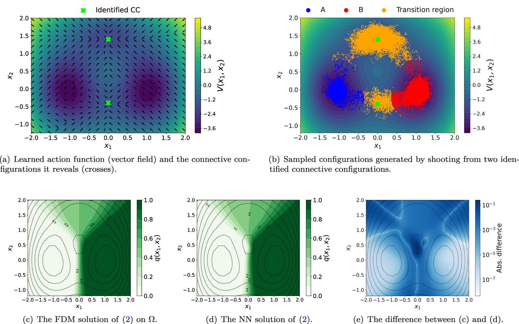
Figure 14. (a) Mean square error of the training loss at configurations sampled from the transition region of the rugged Muller-Brown potential. (b)–(d) NN solutions obtained from different training datasets.
Download figure:
Standard image High-resolution image
From these results, it is evident that the NN solution trained on the dataset generated by shooting trajectories from CC's achieves a lower MSE and yields a more accurate approximation.