Machine learning of hidden variables in multiscale fluid simulation

Machine learning for partial differential equations (PDEs) has received much attention with an emphasis towards computational fluid dynamics [1–4]. Fluid equations describe conservation laws for bulk properties of matter—such as mass, energy, average flow velocity—under the continuum assumption. The equation set usually requires a closure, which involves additional information that represents some 'microphysics' that is not captured by the continuum model. For example, because of turbulence on small scales, or granularity because of the nature of the media being made up of particles/molecules/cells etc an equation may be introduced that represents the relationship between bulk properties, such as a constituent relation (material response to a force) or equation of state (a thermodynamic equation relating bulk properties) While analytic closure models based on equilibrium states have existed at least since the introduction of hydrodynamic equations, the abundance of data and of data-generation mechanisms has prompted a re-examination of the existing methods in light of data-driven models that provide closure for the coupled system of equations. This approach is particularly relevant in systems where physics occurs on length- and time- scales smaller than that which is resolved by the simulations.

Similarly, there are other systems where the fluid approximation itself breaks down because of effects involving an extended phase-space of states; for example, including momentum states where physical effects from the interaction between molecules or particles of a certain velocity become important. In these cases, increasing the resolution of the simulated domain arbitrarily does not recover the missing kinetic physics. Capturing kinetic physics using a first-principles approach requires a fully kinetic description such as solving the Boltzmann equation. Such effects may be included in a fluid model through constituent relations etc that depend on the local conditions that may be derived or learned somehow from a kinetic model or experimental data etc. An example of this is the introduction of modified transport coefficients for nonlocal heatflow in fusion plasma [5]. More recently, the application of machine learning to model turbulence has a growing body of research (see references within [4, 6]).

The issue with any relation derived from local bulk fluid conditions is that it retains no 'memory' of microphysics effects from other locations; the effect is localized in space and time. But it is often the case that nonlocality is important. For example in the case of kinetic flows, fast particle streams will affect transport far, in both time and space, from a region that generates them.

In this article, we expand the method of machine learned closure to learn variables that themselves obey a PDE that describes the space-time variation of the microphysics. We refer to these as 'hidden variables' as they do not describe bulk variables of the fluid system of equations but instead represent some physics that is 'hidden' from the fluid equations. The original term 'hidden variables' was introduced by Bohm to try to explain quantum behavior in terms of some unobservable underlying variables [7]. Here, the meaning is slightly different as although our 'hidden variable' indeed describes physics that is unobservable (within the fluid description), the variable itself is not thought to be fundamental but just an ad-hoc reduced fidelity approximation of the fundamental behavior which can be learned from an ab-initio model. We specifically look at the dynamics of Landau damping of excited plasma wavepackets in the presence of trapped hot electrons, which is described by the higher fidelity Vlasov–Poisson equations. Our fluid model using a Landau closure, similar to that in [8], that is modified to include a hidden variable representing the effect of the hot electron population is able to replicate the fully kinetic behavior. The structure of paper is as follows. Section 2 discusses the inclusion of kinetic effects in a new differentiable fluid simulator using a 'hidden variable' approach. Section 3 introduces the specific problem to address of Landau damping of excited plasma wavepackets and the basic equations to be solved. Section 4 introduces the new 'hidden variable' and its evolution. Section 5 presents the results and comparison with full Vlasov simulation. Finally, we conclude in section 6.

The Boltzmann equation is a PDE that governs the evolution of the distribution function of particles in phase space and is given by

$$\begin{align} \frac{\partial f}{\partial t} + \frac{\mathbf{p}}{m} \cdot \frac{\partial f}{\partial \mathbf{x}} + \mathbf{F} \cdot \frac{\partial f}{\partial \mathbf{p}} = \left(\frac{\partial f}{\partial t}\right)_{\textrm{coll}}, \end{align} \tag{ 1 }$$

where $f = f(t, \mathbf{x}, \mathbf{p})$ is the distribution function in $(\mathbf{x}, \mathbf{p})$ phase space, and F are the forces, and the right-hand-side describes collisional effects. Velocity-space moments of equation (1) give an infinite chain of equations for the conservation of particle density, momentum, and energy. With appropriate closure conditions, these form the Euler equations in the inviscid case, or the Navier–Stokes equations in the viscous regime, depending on the treatment of the collisional term. If the particles are charged, this moment-driven approach gives the plasma fluid equations.

In all cases, the reduction of a three configuration and three velocity phase-space down to a three-dimensional configuration space averages over the details contained in velocity-space. This approximation is justified in systems where the Knudsen number is small such that the particles reach local thermal equilibrium and velocity-space effects, called kinetic effects, are negligible. The Knudsen number is defined by the ratio between the mean-free-path of the particles and the size of the system. There are many important systems where the Knudsen number is not small, and the thermal equilibrium approximation does not hold. For example, in micro- or nano- scale flows where the system size is small, as well as rarified gases such as the high-altitude atmosphere that is experienced by spacecraft where the mean-free-path is large.

In plasmas, kinetic effects are important in the scrape-off layer in magnetic fusion plasmas [5], in the low-density gas-fill in inertial fusion plasmas [5], and in laser- and plasma-based accelerator experiments where the plasma density is low and the physics is weakly-collisional. In such settings, it becomes important to retain the influence of kinetic effects in order to perform accurate modeling of the system dynamics. Another example is in plasma based particle acceleration [9], in particular the phenomena of wavebreaking or trajectory crossing in plasma waves [10]. Fluid simulations of plasma accelerators have the benefit of having smooth distributions compared to typical particle-in-cell simulations, but cannot model crucial electron trapping processes because of phase space mixing.

Previous attempts at the inclusion of kinetic effects into plasma fluid modeling have leveraged analytical methods [8, 11–13]. Modeling kinetic physics using data-driven methods has either been attempted towards benchmarking their performance against known analytical methods [14] or is restrictive in the geometries to which it can be applied [15]. In this work, we develop a machine-learned model that is applied to model a phenomenon with no known analytical representation. It is trained in a small geometry and successfully translated to a much larger domain.

To accurately model the desired kinetic effects in this work, we find that a model that is non-local in space and time is necessary. In other words, we find that memory is required.

To accomplish this, we use an additional transport equation for a hidden variable with learned coefficients for the source term. Because we leverage a hidden variable that can persist over time, it enables the reproduction of the kinetic effect that requires non-locality in time. Since our hidden variable can also be transported, it can be leveraged to reproduce non-local behavior in space. We train the model in a reduced, idealized system against numerical solutions of the collisionless Boltzmann equation. Because our model is a self-consistent system of coupled PDEs with carefully constructed asymptotic behavior, we show that it not only extends to larger systems but can also be used to model phenomena that the neural networks have never previously seen.

In order to maximize the likelihood of developing models that are stable over long time-scales, it is important to develop models either using symbolic or sparse regression techniques [16–18] where the user is able to craft and analyze symbolic formulations and ensure their stability. In the most general case, however, formulating a library of terms that may enable accurate modeling is a challenging task.

Using a function approximator such as a neural network provides a method by which to circumvent that challenge. A useful heuristic is to view purely symbolic and purely data-driven systems as two ends of a continuous spectrum where the variable is different proportions of symbolic and data-driven components [19]. We choose to occupy the part of that spectrum where we impose significant physical constraints through symbolic expressions and judiciously place flexible machine-learned components within those expressions.

The next decision one must make is whether the symbolic expressions must be differentiable or whether the data-driven components can be trained and integrated 'offline'. In the case of simulations, this translates to whether a differentiable simulator (DS) is necessary.

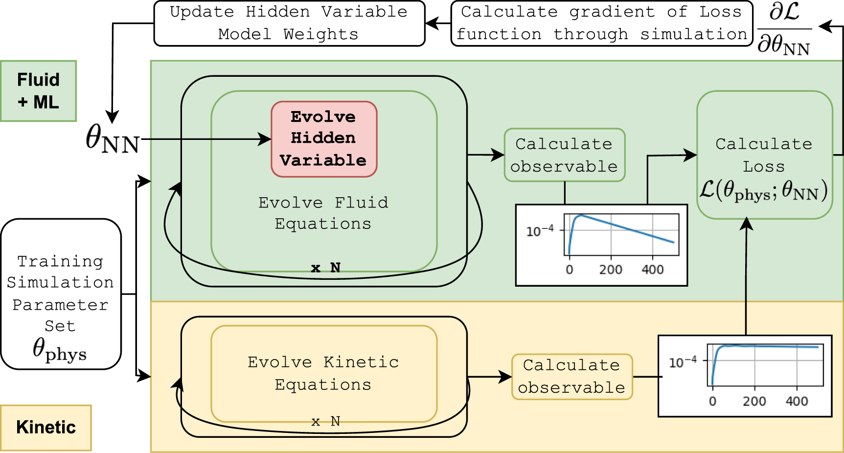
DSs enable the training of neural networks in combination with numerical integration of a dynamical system. DS are not strictly necessary because a neural network may be trained 'offline' and then implemented only using a forward pass in a physics simulator. However, DS enable more flexibility in the set of equations that contain symbolic expressions and neural networks which the user wishes to solve [19, 20]. We exploit this advantage in this work because we seek to implement an additional set of equations for the evolution of a quantity that has no corresponding observables in the training data, that is they are 'hidden'. This paradigm is visualized in figure 1. In this case, an 'offline' supervised training method is not readily available.

Zoom In Zoom Out Reset image size

To enable the use of a quantity for which a model cannot be directly supervised, we choose to develop a differentiable fluid simulator for plasma physics called ADEPT ⁴ . While DSs have been used to construct models for computational fluid dynamics [6, 21–25], and for physics discovery in plasma kinetics [26], to our knowledge, this is the first DS of computational plasma fluid dynamics. The code is publicly available along with the dataset introduced in this work.

Finally, by using a DS, one reduces the number of physical interactions the data driven component must learn as well as numerical properties the data driven component must maintain. This may potentially reduce the required amount of training data. However, we do not test this effect here and calculate the gradient over a large time interval only.

Plasmas are systems where an ionized gas exhibits collective behavior through electrostatic or electromagnetic fields. These fields are capable of sustaining oscillations and waves which leads to a discipline rich in non-linear kinetic behavior. The kinetic behavior arises due to wave-particle interactions, where particles moving at the phase velocity of the wave can exchange energy with the wave. One important example of this is Landau damping [27], where an excited plasma wave will damp even in the absence of dissipative forces. This inherently requires a kinetic description to describe the physics of the wave-particle interaction driven damping mechanism. The linear version of Landau damping can be included via an analytic closure relation, which we do here. We extend that implementation to include the nonlinear version of this effect in a fluid model through the introduction of a 'hidden variable' representing the trapped electron population. We start by describing the simple one dimensional fluid model.

3.1. Fluid model

The relevant equations are the simplest form of the moment equations for electron plasma transport that are necessary for illustrating our method. The nonrelativistic two-moment equations are given by

$$\begin{align} \partial_t n + \partial_x \left(u~n\right) & = 0, \end{align} \tag{ 2 }$$

$$\begin{align} m n \left(\partial_t u + u ~ \partial_x u\right) & = -\partial_x p + q n E, \end{align} \tag{ 3 }$$

where $n = n(t,x), u = u(t,x), p = p(t,x)$ are the density, velocity, and pressure, respectively. We use an adiabatic equation of state as a closure for the equation set,

$$\begin{equation} p = p_0\left(\frac{n}{n_0}\right)^\gamma\;, \end{equation} \tag{ 4 }$$

where $\gamma = (f+2)/f$ is the adiabatic index, with f the number of degrees of freedom, which is set to 3.0 for one-dimensional problems. T is the electron temperature and is assumed to be constant and uniform. $E = E(t,x)$ is the electrostatic field given by solving Poisson's equation, $\partial_x E = (Z n_i - e n) / \epsilon_0$ where n_i is the ion density. Because this problem requires electron timescales, it is satisfactory to assume ions are stationary and form a neutralizing background.

3.2. Base model—linear Landau damping

During linear Landau damping, particles absorb energy from the electric field and are accelerated. Because individual particle trajectories are no longer modeled in the fluid approximation, modeling Landau damping requires a modification to include the microphysics. In [8], a Fourier space operation is used to provide the microphysics closure.

We include Landau damping similarly by adding a damping term to the momentum equation given by equation (3). The modified momentum equation is given by

$$\begin{align} m n \left(\partial_t u + u ~ \partial_x u\right) & = -\partial_x p + q n E + 2 m n~ \nu_L * u, \end{align} \tag{ 5 }$$

where $*$ is the convolution operator defined by $[a*b](x) \equiv \int a(x^{\prime}-x) b(x^{\prime}) \mathrm{d}x^{\prime}$ and ν_L is the wavenumber dependent Landau damping rate. Since ν_L can be calculated for a range of wavenumbers using numerical rootfinders, we pre-compute the ν_L for the computational domain, which serves as a convolutional filter that represents the wave-number dependent damping rate. We verify that this implementation reproduces Landau damping by comparing the results against those from a Vlasov code. We also verify that the analytical linear dispersion relation arising from by equations (2) and (5) recovers the Landau damping rate from the imaginary part of the kinetic dispersion relation.

3.3. Nonlinear Landau damping

When the electric field amplitude is large, particles exchange energy with the electric field, and eventually become trapped in the potential of the wave. The electric field and particles reach a time-averaged steady state during which Landau damping is suppressed and the electric field is not damped. In a weakly-collisional plasma, Landau damping does not completely disappear, but is reduced significantly, and the amount of reduction is a function of the collision frequency, field amplitude, and the wavenumber of the field [28, 29]. This is a distinctly non-linear and kinetic effect that is not captured by the fluid model.

A model equation that enables the field amplitude dependent suppression of Landau damping can be given by

$$\begin{align} m n \left(\partial_t u + u ~ \partial_x u\right) & = -\partial_x p + q n E + 2 ~ mn~\nu_L\left(k, \nu_{ee}, |E|^k; \theta_\textrm{NN}\right) * u, \end{align} \tag{ 6 }$$

where k is the wavenumber, ν_ee is the electron–electron collision frequency, and ν_L is now a function of the wavenumber dependent field amplitude, $|E|^k$. An analytical solution for ν_L is not available, but a representation can be machine learned via tuning its weights and biases, θ_NN.

However, it has been shown that this model for nonlinear Landau damping is inadequate because it does not capture the kinetic effects due to the excited resonant electrons. The following section describes this in more detail.

3.4. Motivating non-local physics through wavepacket etching

3.5. A spatiotemporally non-local model of Landau damping

We modify equation (6) by adding an auxiliary 'hidden variable' $\delta = \delta(t,x)$ that represents the resonant electrons. From this section on we write the equations in normalized form using electrostatic units where $v\rightarrow v / v_{th}$, ${x} \rightarrow x/\lambda_D$, $k \rightarrow k\lambda_D$ ${t} \rightarrow \omega_p t$, ${m} \rightarrow m/m_e$, ${q} \rightarrow q / e$, and ${E} \rightarrow e E / m_e v_{th} \omega_p$ [26]. Here, v_th is the thermal velocity, ω_p is the plasma frequency, and m_e , and e, are the electron mass, and charge, respectively. Since we seek to minimize Landau damping in their presence, we assume a sigmoidal dependence, similar to that in [31, 32], and the resulting momentum equation is given by

$$\begin{align} m n \left(\partial_t u + u ~ \partial_x u\right) & = -\partial_x p + qnE + 2 ~ mn ~ \frac{\nu_L * u}{1 + \delta^2}. \end{align} \tag{ 7 }$$

The growth and transport of δ is given by

$$\begin{align} \partial_t \delta & = v_{ph} \partial_x \delta + \nu_g ~ \frac{|E * \nu_L|}{1+\delta^2}, \end{align} \tag{ 8 }$$

$$\begin{align} \nu_g & = \nu_g\left(k, \nu_{ee}, |\hat{E}^k|; \theta_g\right). \end{align} \tag{ 9 }$$

This model makes use of the knowledge that, since δ represents the electrons in phase with the wave, δ must be transported at the phase velocity. Because δ is initialized at zero, the proportionality factor of the source term is what is approximated via a machine learned function.

To understand why we choose this specific formulation of the source term, we start with equation (1), and assume dynamics in the non-relativistic limit, $\mathbf{p} = m\mathbf{v}$ as a result of an electrostatic force, $\mathbf{F} = \mathbf{E}$, and small-angle collisions that result in drag and diffusion of the electrons and reduce the system to a one spatial and one velocity dimension (1D-1V) with periodic boundaries in the spatial direction. This results in the well-known and long-established 1D-1V Vlasov–Fokker–Planck [33, 34] equation set which is given by

$$\begin{align} \partial_t f + v ~ \partial_x f + E~ \partial_v f & = \nu_{ee} ~ \partial_v \left(vf + v_0^2 ~ \partial_v f\right), \end{align} \tag{ 10 }$$

$$\begin{align} \partial_x E & = Z n_i - n_e, \end{align} \tag{ 11 }$$

where $f = f(t, x, v)$ is the electron distribution function, Z = 1 is the atomic charge, and $n_i = 1$ is the ion density. This set of equations, in varying forms, applies to plasmas as well as gravitational systems [35, 36].

The third term on the left hand side of this equation describes how the wave and particles interact. For example, consider that the energy moment of the third term in equation (10) is $\int \mathrm{d}v ~ v^2 ~ E \partial_v f = j ~ E$ which allows for energy exchange between kinetic and potential energy. This term is the reason why we use $E ~ \nu_L$ in the source term. Landau [27] determined $\partial_v f \propto \nu_L$. Assuming this proportionality, and restricting ourselves to the electrostatic force, the third term in equation (10) can be written as $E ~ g(\nu_L)$. Absorbing the g function into ν_g gives us $\nu_g |E * \nu_L|$.

Finally, we wish to create an asymptotic relation where as δ grows, the source term decreases. This is because the wave-particle interaction is known to saturate after a short period of time given a finite amount of wave energy. This is also the reason why δ represents the particles that are resonant with the wave.

4.1. Acquiring kinetic simulation data

The kinetic nonlinear physics that we seek to learn is contained within simulation data collected from solving equation (10). In all simulations, we simulate a wave with the wavelength equal to the box length. We limit ourselves to a single wavelength excitation because capturing the richness of nonlinear wave-wave and wave-particle effects that can arise due to multiwavelength excitations in plasmas is outside the scope of this work. Furthermore, in typical inertial-fusion relevant laser-plasma interaction experiments, the coupling is sufficiently narrowband where the dynamics can be described by single wavelength systems to zeroth order.

The parameters of the temporal envelope of the external forcing term are $t_w = 40 \omega_p^{-1}, t_r = 5 \omega_p^{-1},$ $t_c = 40 \omega_p^{-1}$. The implementation of the forcing term is given in [26] and more details for this solver are given in [26, 37].

From each simulation, the key observable that we wish to train our fluid model is given by the first order density perturbation, $\hat{n}^1$. This is a quantity that is damped via the inherently kinetic Landau damping mechanism, and at large amplitudes, displays nonlinear effects. Therefore, it carries the nonlocal kinetic physics that we wish to replicate via our fluid model and is the quantity against which the fluid model is supervised. A few examples are shown in figure 2.

Zoom In Zoom Out Reset image size

The full dataset comprises 2535 first-principles simulations. The parameters that are varied are given by

$$\begin{align} \nu_{ee} \in \left[10^{-7}, 10^{-6.666}, 10^{-6.333}, 10^{-6}, \ldots, 10^{-3}\right], \end{align} \tag{ 12 }$$

$$\begin{align} k \in \left[0.26, 0.27, 0.28, \ldots, 0.4\right], \end{align} \tag{ 13 }$$

$$\begin{align} a_0 \in \left[10^{-6}, 10^{-5.666}, 10^{-5.333}, 10^{-5}, \ldots, 10^{-2} \right]. \end{align} \tag{ 14 }$$

Out of this, we subsample a 200 simulation training and validation dataset given by

$$\begin{align} \nu_{ee} \in \left[10^{-7}, 10^{-6}, 10^{-5}, 10^{-4}, 10^{-3}\right], \end{align} \tag{ 15 }$$

$$\begin{align} k \in \left[0.26, 0.28, 0.3, 0.32, 0.34, 0.36, 0.38, 0.4\right], \end{align} \tag{ 16 }$$

$$\begin{align} a_0 \in \left[10^{-6}, 10^{-5}, 10^{-4}, 10^{-3}, 10^{-2} \right]. \end{align} \tag{ 17 }$$

We split this dataset with a $90\%/10\%$ split. For this dataset, training in parallel over 20 compute nodes takes about 30 min an epoch. See section 5.4 for more details on the compute and data utilization.

$\hat{n}^1$ is the observable we seek to emulate with the fluid equations but we have chosen to modulate $n(t, x)$ with $\delta(t, x)$. However, δ is not a quantity that can be directly extracted from the kinetic code and therefore, needs 'indirect' supervision through a differentiable simulator.

4.2.  ADEPT—Automatic-differentiation-enabled plasma transport

As motivated earlier in the manuscript, because we do not have the ability to directly supervise against our 'hidden' variable, to train the model in equation (9), we need a simulator that can model the set of equations given by

$$\begin{align} \partial_t n + \partial_x \left(u~n\right) & = 0, \end{align} \tag{ 18 }$$

$$\begin{align} m n \left(\partial_t u + u ~ \partial_x u\right) & = -\partial_x p + q nE + 2 ~ mn ~ \frac{\nu_L * u}{1 + \delta^2}. \end{align} \tag{ 19 }$$

$$\begin{align} p & = n^\gamma, \end{align} \tag{ 20 }$$

$$\begin{align} \partial_x E & = \frac{q}{m}\left(n-1\right), \end{align} \tag{ 21 }$$

$$\begin{align} \partial_t \delta & = v_{ph} ~ \partial_x \delta + \nu_g ~ \frac{|E * \nu_L|}{1+\delta^2}, \end{align} \tag{ 22 }$$

$$\begin{align} \nu_g & = 10\,^{f\left(\tilde{E}_k, \tilde\nu_{ee}, \tilde k; \theta_g\right)}, \end{align} \tag{ 23 }$$

$$\begin{align} f\left(E, \nu_{ee}, k; \theta\right) & = 3\tanh\left(g\left(\tilde \nu_{ee}, \tilde k, |\hat{\tilde{E}}^k|; \theta\right)\right), \end{align} \tag{ 24 }$$

where the final term in equation (19) represents the non-local kinetic effect that is added to the typical Euler equations. The closure relation for that term is given by equations (22)–(24) where ν_g is the key coefficient that must be learned from data.

4.2.1. Neural network details and input normalization

$g(\tilde \nu_{ee}, \tilde k, |\tilde{E}^k|; \theta)$ in equation (24) is the function representing the output from a feedforward neural network with a depth of 3 and width of 8 units. The intermediate activation function is the hyperbolic tangent function. To decrease the chances that the growth rate does not result in numerical instability, we bound the growth rate so that $10^{-3} \lt \nu_g \lt 10^{3}$ by leveraging the properties of the hyperbolic tangent.

$\tilde{\nu}_{ee} = \left(\log_{10}(\nu_{ee}) + 7\right)/4$ is the normalized electron-electron collision frequency, $\tilde{k} = (k - 0.26) / 0.14$ is the normalized wavenumber, $|\hat{\tilde{E}}^k| = (\log_{10}(|\hat{E}^k| + 10^{-10}) + 10 ) / -10$ is the normalized value of the electric field amplitude of the kth mode number. We choose this formulation for normalizing the electric field to avoid possible problems with taking the logarithm of zero.

4.2.2. Solver and simulations

We solve this set using a pseudo-spectral, finite-volume method with a fourth order time-stepper [38] in a spatially periodic domain. The gradients are computed using Fourier transforms. Similarly, Poisson's equation is also solved spectrally. All the other operations, e.g. advection, are performed in real space.

The length of the box is given by the wavenumber being sampled because $L = 2\pi / k$. We run the simulation for $500 \omega_p^{-1}$ with $N_t = 10\,000$ timesteps. The forcing function parameters and all other parameters are the same as those used in the kinetic simulations.

4.2.3. Fluid modeling

The fluid simulations used for training the model have different spatial and temporal resolutions, given by $N_x = 16, \Delta t = 0.025$, but are performed over the same spatial and temporal domains as the kinetic simulations.

Since we seek to replicate the behavior of an electron plasma wave with our fluid model, our training objective function is to minimize the mean squared error between the timeseries from the Vlasov and fluid simulations. Formally, the loss function is given by

$$\begin{align} \theta_\textrm{phys} & = \left(a_0, \nu_{ee}, k \right) \end{align} \tag{ 25 }$$

$$\begin{align} \mathcal{L} & = \left[\frac{1} {N_t}\sum_{t = 250 \omega_p^{-1}}^{450 \omega_p^{-1}}\left(\log_{10}|\hat{n}^{1}_{f}|\left(\theta_\textrm{phys}; \theta_{NN}\right) - \log_{10}|\hat{n}^{1}_V\left(\theta_\textrm{phys}\right)|\right)^2\right], \end{align} \tag{ 26 }$$

where θ_phys is the parameter vector that consists of unique combinations of the parameters listed in equations (15)–(17), $|\hat{n}^{1}|$ is the time history amplitude of the first mode of the density profile with the subscripts of f and V correspond to fluid and Vlasov, respectively. It is important to note that we compare the logarithm of the timeseries in the loss function. This is because the wave amplitude can be damped over many orders of magnitude. Without leveraging the logarithm, the wave amplitudes at the end of the simulation will be negligible in comparison to that near the beginning and would effectively be ignored by the gradient descent algorithm.

In this section, we will discuss the performance of the trained model on the training set as well as the test set. We will not compare the performance with respect to other models or baselines because all previous models in the literature, for example [28, 31, 39], have either only been tuned to one simulation or have only been calculated in the large amplitude limit and are therefore, invalid for many of the simulations tested here. An analytical model could be constructed by combining the techniques described in the above references but this has not been done before, and is a substantial undertaking that is outside of the scope of this work. In fact, we believe this is the first published model for weakly-collisional nonlinear Landau damping that can span over a range of amplitudes, collisionallities, and wavenumbers relevant to inertial fusion experiments.

The primary quantitative details associated with the training process are aggregated and provided in table 1, and also discussed in the next few sections. We experimented with a few hyperparameter combinations before we converged on the ones in table 1 here. Using ReLU as the intermediate activation function was not as performant as using tanh. Experiments with larger learning rates of 0.1 also did not perform as well as 10⁻³ did. We did not find a need to try different model architectures because we want to take a gradient through thousands of timesteps and therefore, wanted to keep the network relatively small.

Table 1. The details associated with the training process, the neural network, and the compute requirements are aggregated and provided here.

Epochs	27
Batch size	20
Learning rate	$4 \times 10^{-3}$
Feedforward network depth	4
Feedforward network width	8
Feedforward network parameters	160
Feedforward network intermediate and final activation	tanh
Train set size	200
Validation set size	20
Test set size	2335
Train loss	$5.8 \times 10^{-3}$
Val loss	$2.0 \times 10^{-2}$
Test loss	$1.0 \times 10^{-2}$
Time per training step	50 s
Time per kinetic simulation	210 s (GPU)
Time per fluid+ML simulation	15 s (CPU)

Then we will discuss the evaluation of the trained model on a system with a much larger geometry of $\mathcal{O}(100)$ wavelengths rather than 1. In the previous system, a single wavelength wave is excited in a periodic box of one wavelength in length. In the new system, the wave is driven over 10 wavelengths and is then allowed to propagate freely. We find that the model with the δ physics is able to replicate the true kinetic behavior of the system where a naive local model fails.

5.1. Training set

In figure 3, we show the mean squared error over the training epochs for training and validation. We implement data parallel training by running $N_\textrm{batch}$ simulations in parallel and averaging their gradients on the primary node that is running the optimization algorithm. We use ADAM with a learning rate of 0.004 as the optimization algorithm. We stop training after the performance has saturated for many epochs.

Zoom In Zoom Out Reset image size

Figure 4 shows the result of two sample simulations. We choose to show the result of these two sets of parameters because they are representative examples of two extremes that the machine learning model must be able to handle.

Zoom In Zoom Out Reset image size

In figure 4(a), we show the results from a simulation with $\nu_{ee} = 10^{-6} , k = 0.34, a_0 = 10^{-6}$. The two simulations agree well. This is a parameter regime where linear Landau damping is expected, and therefore, the theory from section 3.2 applies. Therefore, theory dictates that to reproduce the desired behavior, δ must remain small. Figure 4(b) shows that $\delta \approx 10^{-5}$ as the theory suggests it should. Because we train using the logarithm, as stated in equation (26), we are able to capture the damping over five orders of magnitude.

In figure 4(c), we show the results from a simulation with $\nu_{ee} = 10^{-5}, k = 0.32, a_0 = 10^{-2}$. The two simulations agree well. In this parameter regime, kinetic theory dictates that there is a complex interplay between the collisions, represented by ν_ee , and the field amplitude, represented by a₀. Here we expect that to reproduce the desired behavior, δ must be some finite quantity that appreciably, but not completely suppresses the damping. Figure 4(d) shows that δ ≈ 7 and the damping is suppressed by a factor of 50.

5.2. Test set

In this section, we evaluate the performance of the trained model on the test dataset. Since the test inputs are all interpolations of the training data, and since there are nearly an order of magnitude more test data, it is useful to visualize the error distributions on the training and test inputs as shown in figure 5.

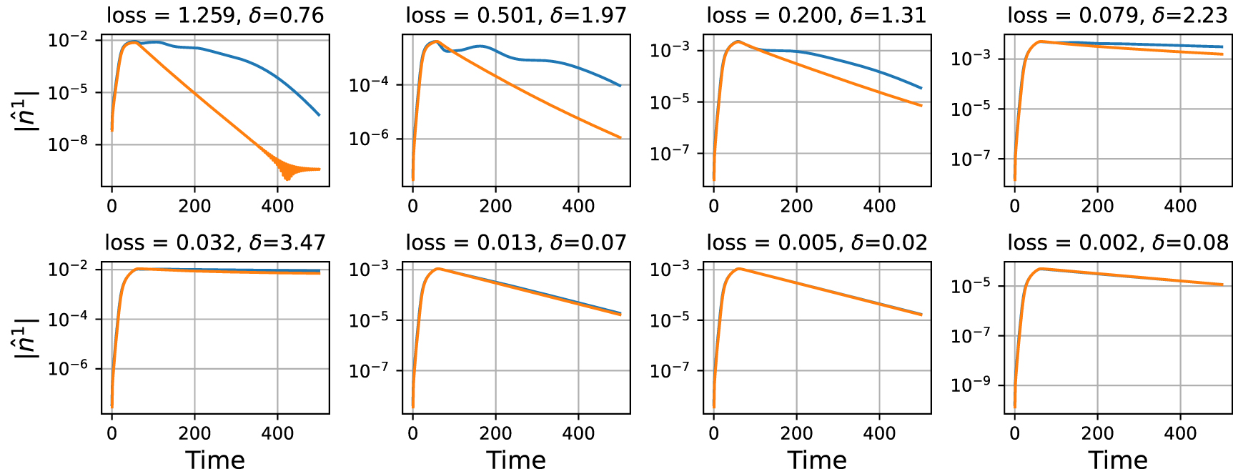
Zoom In Zoom Out Reset image size

We also show the results of individual simulations from various error bins from figure 5 in figure 6. We see that the model performs well for a range of δ, that is, it is able to capture nonlinear effects and is able to maintain a small δ in case the situation calls for a linear treatment.

Zoom In Zoom Out Reset image size

Now that we have been able to learn a microphysics model, we use the coupled set of PDEs along with the newly acquired model weights to simulate a novel geometry and verify its performance qualitatively.

5.3. Extending to larger geometries

In the previous section, we trained on a dataset of systems where a single wavelength wave was excited in a box of one wavelength in length. To assess the performance of our learned model in unseen geometries, we perform simulations where the box size is increased by a factor of 100 and a 20 wavelength long, finite-length wave is modeled. This tests the ability of the machine learned model combined with the hidden variable approach that was trained on a limited geometry to generalize to larger length scales and different boundary conditions. To verify the fidelity, we compare the results of the learned fluid simulations to their kinetic counterparts acquired by using the Vlasov–Boltzmann solver.

As discussed in 3.4, it was shown in [26, 30] that finite length wavepackets damp non-uniformly. The non-uniformity arises because resonant electrons that are responsible for the loss of damping travel faster than the wave. The difference in speeds causes the wave to damp less in the front of the wave than in the back. It is also important to note that the importance of the difference in speeds for different populations of particles means the phenomenon is inherently kinetic. In a single wavelength periodic system such as that in the training set, this phenomenon is muted because the resonant particles can never actually get ahead of the wave. In a many wavelength long system with a finite wave, we expect this phenomenon to occur and it provides a good test of generalizability for the set of equations we have chosen and the coefficient function we have learned because the construction of equation (22) is what enables dynamics at different speeds in the fluid simulations.

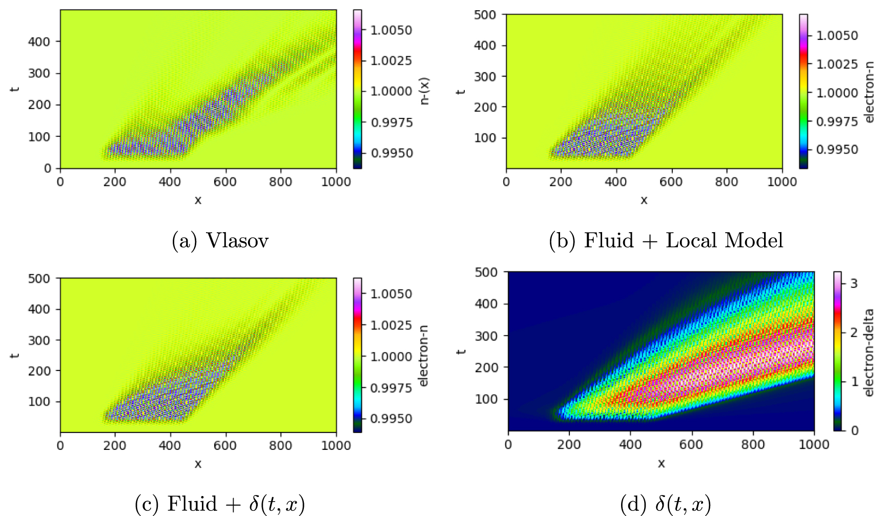
In figure 7(a), we show an example of this phenomenon. Figure 7(b) shows that if a local implementation of Landau damping is used, for example, like the one given by equation (6), the non-uniform damping will not be reproduced because the damping rate will be the same along the length of the wavepacket. In contrast, figure 7(c) shows that the implementation using the machine-learned dynamical hidden variable approach is much more capable of reproducing the results from the ab-initio simulation. Figure 7(d) confirms that δ grows to account for the suppressed damping, and then is transported to account for the non-locality in space and time.

Zoom In Zoom Out Reset image size

Similar to that in figure 4, we also show the behavior in the linear regime exemplified by a small amplitude simulation in figure 8(a). In this regime, it is expected that Landau damping remains local as shown in figure 8(b). Figure 8(d) shows that the model does not anomalously generate large δ. Because of this, in figure 7(c), we see that linear Landau damping proceeds as expected and the non-local model recovers the local result.

Zoom In Zoom Out Reset image size

In this work, we seek to highlight the fact that because we choose to embed the machine learning model into a set of coupled PDEs that are capable of generalizing, we can train the model on a simple system and can scale the learned physics to a significantly more complex domain. In this case, we scale a single wavelength periodic system to a finite-length wavepacket in an open boundary simulation but this model could be very well be extended to multiple spatial dimensions. If the use-case were to acquire as accurate a model as possible in order to perform multi-scale modeling of an actual experiment, one could and should train the model on as many geometries as is feasible.

5.4. Compute and data costs

The marriage of numerical PDE solvers and deep learning driven models is more than coincidental because they are both products of numerical computing. The advent of scalable and performant scientific computing libraries that are capable of automatic differentiation, e.g. JAX and Julia, has enabled a seamless interchange of ideas between the two paradigms where the lines between each continue to blur.

In this work, we show how the two paradigms can be intimately woven together and leveraged towards performing multiscale modeling where the equation set does not natively contain all the necessary microphysics, and where the microphysics model itself has proven to be challenging to construct using conventional methods. By training against a dataset with a relatively simple geometry and parameters, we are able to learn a model that can emulate spatio-temporally non-local physics over broad parameter ranges and geometries, physics which can otherwise only be described by computationally expensive higher-dimensional PDE solvers. The key to preserving the spatio-temporally non-local dynamics is providing a dynamical system for a hidden variable that governs the physics. By allowing for growth and transport of the hidden variable, we enable non-locality in time and space. Furthermore, the proposed method is an example of how differentiable simulations enable 'indirect' supervision of non-observable, hidden variables.

We envision that a model that leverages machine-learned hidden variables can be used for various phenomenon inside and outside of plasma physics. For example, hot electrons created from laser-plasma instabilities are deleterious towards successful fusion experiments. Accurate modeling of their dynamics and energetics in fully integrated hydrodynamics simulations of fusion experiments can help substantially improve the predictive power of simulations and improve the results of fusion experiments.

We acknowledge funding from the DOE Grant # DE-SC0016804.

We acknowledge that this material is based upon work supported by the Department of Energy National Nuclear Security Administration under Award No. DE-NA0003856, the University of Rochester, and the New York State Energy Research and Development Authority through a subcontract between Ergodic, L.L.C. with the Laboratory of Laser Energetics at the University of Rochester.

This report was prepared as an account of work sponsored by an agency of the U.S. Government. Neither the U.S. Government nor any agency thereof, nor any of their employees, makes any warranty, express or implied, or assumes any legal liability or responsibility for the accuracy, completeness, or usefulness of any information, apparatus, product, or process disclosed, or represents that its use would not infringe privately owned rights. Reference herein to any specific commercial product, process, or service by trade name, trademark, manufacturer, or otherwise does not necessarily constitute or imply its endorsement, recommendation, or favoring by the U.S. Government or any agency thereof. The views and opinions of authors expressed herein do not necessarily state or reflect those of the U.S. Government or any agency thereof.

We use and would like to acknowledge open-source software from the Python ecosystem for scientific computing. Specifically, we use NumPy [40], SciPy [41], matplotlib [42], Xarray [43], JAX [44], and Diffrax [45] while the neural network is managed using Equinox [46]. The numerical experiments and data are managed using MLFlow [47] as discussed in [48].

A J also thanks D J Strozzi and W B Mori for useful discussions.

The data that support the findings of this study are openly available at the following URL: https://github.com/ergodicio/adept.

Authors declare no competing interests.