
Abstract
The phenomenal success of physics in explaining nature and engineering machines is predicated on low dimensional deterministic models that accurately describe a wide range of natural phenomena. Physics provides computational rules that govern physical systems and the interactions of the constituents therein. Led by deep neural networks, artificial intelligence (AI) has introduced an alternate data-driven computational framework, with astonishing performance in domains that do not lend themselves to deterministic models such as image classification and speech recognition. These gains, however, come at the expense of predictions that are inconsistent with the physical world as well as computational complexity, with the latter placing AI on a collision course with the expected end of the semiconductor scaling known as Moore's Law. This paper argues how an emerging symbiosis of physics and AI can overcome such formidable challenges, thereby not only extending AI's spectacular rise but also transforming the direction of engineering and physical science.
Export citation and abstract BibTeX RIS

Original content from this work may be used under the terms of the Creative Commons Attribution 4.0 license. Any further distribution of this work must maintain attribution to the author(s) and the title of the work, journal citation and DOI.
1. Introduction
In the midst of the race to put a man on the moon in the 1960s, the Kalman filter performed the crucial task of estimating the trajectory of the Apollo spacecraft to the moon and back. With crude computers and imperfect sensors and with the lives of astronauts at stake, neither physics models nor sensor data alone could be relied on for accurate navigation. The Kalman filter is an early example of how blending physics and data-driven models can solve critical problems in resource constrained and data starved applications [1].
Physics and data-driven models represented by artificial intelligence (AI) are two extremely different approaches to modeling the world. AI is an empirical method and is how science was pursued in the early days before we had accurate instruments to measure and quantify natural phenomena and advanced mathematical tools (calculus, differential equations etc) to model them. In those days, science was empirical as exemplified by alchemy. Models were deduced from results of trial and error, forming empirical laws which were a mix of facts and superstition. The beliefs were data-driven and based on observations without rigorous mathematical formulations.
Humanity then entered the era of physics with deterministic models based on first-principle. Using only a few physically quantifiable parameters such as mass, charge and distance, these models can explain a vast range of phenomena. Such mechanistic models in their native form (physics) or higher-level abstraction (chemistry, biology) have been the foundation of scientific and technological advancements.
Today, AI and in particular deep neural networks (DNNs) are revolutionizing computer vision (CV) and natural language processing (NLP). For problems such as image classification and detection, neural networks can even outperform humans [2]. Remarkably, these deployed AI algorithms are able to succeed without a priori structures built into their designs; instead, they leverage billions, sometimes even trillions, of free parameters that adapt to data. Unfortunately, learning the correct setting of these free parameters means that the contemporary paradigm of neural networks requires massive datasets which are not available in many domains such as medical diagnostics [3]. These free parameters constitute a black box and it is difficult for such neural networks to offer interpretability and robustness guarantees. Furthermore, the current trajectory of neural networks where performance gains are obtained by the increase in network size is further challenged by the fundamental scaling limits of semiconductor technology known as Moore's Law. We would like to point the readers to the seminal review article [4] and textbook [5] as references for introduction and tutorial of neural networks and deep learning. Therefore, we will not cover the basics of neural networks in this paper given the limited space.
Now there is growing conviction in favor of hybrid approaches where laws of physics and physical systems merge with AI to enable better inference, prediction, vision, control and more [6, 7]. In this new paradigm both scientific and data-driven models are integrated in a synergistic manner. This approach allows forward and inverse simulations of fluid dynamics and quantum simulations where it is computationally infeasible to run deterministic models. AI models can now be used in domains where large datasets for training are not available. Physically consistent results that better generalize to out-of-sample scenarios can be obtained.
We refer to this new age as the 'Physics-AI symbiosis' as shown in figure 1. A mix of perspective and review, the present paper explores emerging techniques in which physics is blended with AI to extend the capabilities of either approach. We see three emerging categories and organize the paper accordingly: (a) AI replaces physics models. The laws of physics are used as priors to enhance neural networks that become efficient substitutes for the finite-element and finite-difference physics models. And neural networks are also being explored to learn both numerical relations and intuition about the physical world. (b) Physics as a computer, where physical systems substitute numerical models to accelerate computations, (c) Physics inspired algorithms, where algorithms emulate physical laws. Finally, applications that will be transformed by these techniques, such as drug discovery and climate modeling are discussed in section 5.
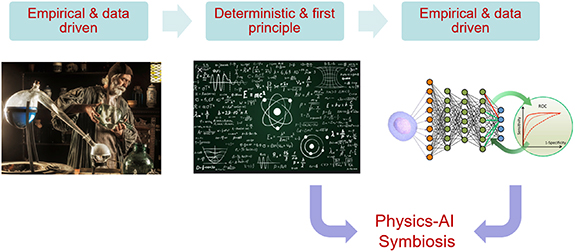
Figure 1. The evolution of science spans the data-driven empirical age of alchemy followed by first-principle deterministic age of physics to the new age of empirical data-driven neural networks powered by mighty computers and big data. Physics-AI symbiosis represents the marriage of empirical and mechanistic models with the aim of providing the best of both worlds.
Download figure:
Standard image High-resolution image2. AI replaces physics models
Filling the gap between purely physical models and empirical data-driven approaches, physics-based learning is currently undertaking a quest for a unified approach that can blend physics and learning. Such an approach would be able to handle variations in the quality of the physical prior and the dataset, enabling the algorithm to generalize across a range of physical problems.
2.1. AI accelerates computation of master equations of physics
One emerging trend in blending physics and learning, is to use DNNs as computationally efficient surrogates for partial differential equations (PDEs) of physics, an approach that accelerates the forward simulations and inverse design used in optimization of engineered physical systems. One example is computing the transmission spectra of a metasurface, an artificial 2D structure with subwavelength features, given its geometry. This involves long computing times necessary to numerically solve the Maxwell's equations in complex structures. It is now possible to train a generative model with a simulator (S), a generator (G), and a critic (D) to inversely design metasurface patterns according to the desired optical spectra [8]. While training such a generative model is time consuming, once trained, it becomes a numerically fast substitute model for the Maxwell equations. The need for training data can be avoided by utilizing a physics driven loss as explained later [9]. Recently, a model called MaxwellNet is proposed [10, 11]. MaxwellNet can approximate solutions to Maxwell's equations without relying on large training datasets that would have to be experimentally or computationally generated [10]. This results in up to 1000 times faster simulation time than the popular COMSOL Multiphysics solver [12]. Similarly, modeling fluid flow is one of the major challenges in computational physics, with diverse applications in weather forecasting and aerodynamics. Recent work has shown that instead of modeling such flow with Navier–Stokes equations, one can directly train a DNN with training datasets from real life experiments [13]. Once trained, the DNN provides high fidelity predictions. Another example involves nonlinearity compensation in optical data communication networks. Modeling optical nonlinearities requires solving the nonlinear Schrödinger equation (NLSE) using split-step Fourier method (SSFM) [14]. However, the iterative process in SSFM is time-consuming. Recent work has shown that a neural network emulates the SSFM but runs much faster. Such a neural network has several blocks that operate on the complex electric field, each block consists of a 1D convolution layer that mimics dispersion and a customized activation layer that provides nonlinearity. In one implementation, this neural network has achieved 18 dB signal to noise ratio with 4 dBm transmit power in 16-QAM transmission [15]. The main challenge with equalization of data in optical network is real-time execution of the algorithms at ultrahigh data rates. Neural networks may have the potential for real-time operation at optical communication data rates [16]. The last example is about solving problems in quantum chemistry. The potential energy surface is the central quantity of interest in modeling of molecules and their interaction. However, it is costly to compute the potential energy from the Schrödinger equation. OrbNet is a graph neural network that uses atomic-orbital features to predict the solution of the Schrödinger equation. It achieves similar accuracy compared to the density functional theory but with a computational cost that is reduced by several orders of magnitude [17]. In the original demonstration, it outperforms other deep learning methods by achieving MAE of 6.8 meV (mean square absolute error in energy) on the QM9 dataset [18] with 50 000 training samples.
2.2. AI as general PDE solvers
While efforts have been made to design neural networks for solving specific types of PDEs, a more ambitious attempt is to develop a general neural network architecture that can learn different types of PDEs. Current work on neural networks as general PDE solvers can be divided into the following two approaches. Figure 2 compares the two approaches based on a ubiquitous PDE utilized in fluid dynamics called Burgers' equation. It is characterized by parameters  and
and  , initial condition
  and periodic boundary conditions, and the domain of variables as shown below. Its solution
  depends on the spatial variable
  and the temporal variable
  :
:

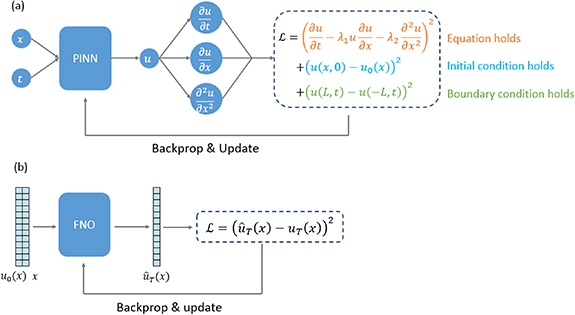
Figure 2. Comparison of two approaches to neural network based PDE solvers. (a) Physics-informed Neural Network (PINN) solves one instance of PDE at all points in the defined domain with fixed parameters, initial and boundary conditions. The network is guided by a physics-driven loss, defined as the residual of the prediction relative to the physical differential equation including the initial and boundary conditions. (b) Fourier Neural Operator (FNO) learns the mapping from different initial conditions to corresponding solutions at time  for different instances of PDEs, defined as fixed parameters and boundary conditions but with different initial conditions.
Download figure:
Standard image High-resolution imageThe first approach trains a neural network to learn a given instance of PDE at all points in the defined domain. An instance of PDE is defined as a PDE with fixed parameters ( and
and  , and fixed initial and boundary conditions. Physics-informed neural network (PINN) [9] shown in figure 2(a) is a pioneering example of such an approach. The second approach trains a neural network to solve different instances of PDEs by learning the mapping from the initial condition to the solution at a specified time
  . Different instances of PDEs are defined as PDEs with fixed parameters (
 and
and  and boundary conditions but different initial conditions
  . Fourier neural operator (FNO) [19] shown in figure 2(b) is a representative work of such an approach. Below, these two approaches are explained further.
PINN [9] utilizes a physics-driven loss defined as the residual of the network prediction relative to physical differential equation including the initial and boundary conditions. It solves an instance of PDE with fixed parameters, initial and boundary conditions. It takes scalar values (single point) of spatial and temporal coordinates  as input and approximates the solution
  at the corresponding coordinate. Since the parameters, initial and boundary conditions of the PDE are fully known, it does not need training datasets. Training can be done by sampling
  in the defined domain and using loss derived from the equation itself as well as its initial and periodic boundary conditions as shown in figure 2(a). Once trained, the PINN can solve the given PDE at any point in the defined domain. Besides Burgers' equation, it has also been successfully applied to solve NLSE, Navier–Stokes equation, etc. Quantitatively, the relative
  error (between predicted and exact solution) is 0.2% when solving the NLSE by a five-layer fully connected neural network with 100 neurons per layer, the relative
  error is 0.06% when solving the Burgers' equation by a six-layer fully-connected neural network with 40 neurons per layer [9]. One limitation of this approach is that the trained network solves only a single instance of the PDE with a fixed set of parameters and conditions. It cannot generalize to other instances in the same PDE family. When parameters or initial and boundary conditions change, the network has to be re-trained. This is impractical for applications where solutions to the PDE are required for various instances.
A neural operator learns the mapping from different initial conditions to corresponding solutions at time  as shown in figure 2(b). It is trained in a supervised manner with the dataset
  , where
  is an instance of the initial condition and
  is the corresponding solution at time
  and
and  is the set of spatial coordinates. The solution of the PDE is approximated with a cascade of layers each containing linear and nonlinear transformations. Fourier Neural Operator (FNO) [19] performs these in the Fourier space as shown in figure 3. It takes an array of coordinates
  and the corresponding initial condition
  and lifts them to a higher dimensional space by an encoder network
  . The high dimensional representation
  goes through the cascade of layers each consistent of two paths. In the upper path input is first transformed into the Fourier space, then low frequency components are kept and re-weighted by channels while high frequency components are truncated. The features in the Fourier space are transformed back to the original space by an inverse Fourier transform. The lower path performs a linear transform in the original space. The sum of the two paths goes through a nonlinear operation (activation). At the output, the high dimensional representation
  is projected back to the target dimension by a decoder neural network
  which gives the solution
  at time
  . A loss function defined as the difference between the predicted solution
  and the ground truth
  is applied. Once trained, FNO is able to solve the given PDE with unseen initial conditions. It has been applied to solve 1D Burgers' equation based on the aforementioned settings and has also been extended to solve 2D Darcy Flow and Navier Stokes equation. It has been reported that FNO can achieve 1.5% relative
  error in solving Burgers' equation and 1% for solving 2D Darcy Flow while being up to three orders of magnitude faster compared to traditional PDE solvers [19]. Furthermore, by operating in the Fourier domain, FNO can be directly evaluated on a higher resolution sampling grid by only being trained on lower resolutions [19]. Unlike the PINN, this approach requires training datasets.
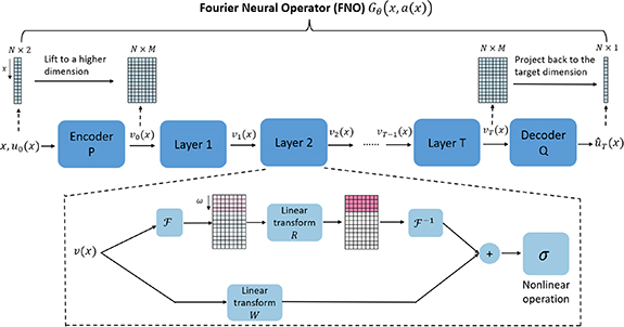
Figure 3. The diagram of FNO. PDEs govern fundamental physical phenomena such as fluid dynamics and electromagnetics. FNO learns the solution of different instances of PDEs. Different instances are defined as PDEs with fixed parameters and boundary conditions but different initial conditions. FNO is trained on the input (the PDE initial condition  ) concatenated with the spatial coordinates
  ), and output (the PDE solution
  ) pairs [19]. The input is first encoded into a high dimensional space. It then propagates through a sequence of layers each consisting of a linear transformation and a nonlinear operation. The linear stage consists of an upper path performing filtering and a lower path which applies weights. Finally, the high dimensional representation is projected back to the target dimension of the solution. This architecture is able to learn the general behavior of PDEs.
Download figure:
Standard image High-resolution image2.3. Physics neural architecture search
Besides being blended into neural networks for efficiently solving PDEs, physics priors have also been exploited in identifying the optimal architecture by searching over a topological space of neural network configurations. This algorithm, dubbed PhysicsNAS (Physics neural architecture search), is able to blend physics and learning for problems such as collision estimation and projectile motion [20]. In particular, to blend prior equations into the network, PhysicsNAS has a physics-only branch, which takes as input the kinematic equations. One can envision PhysicsNAS as a form of multimodal fusion, where physics is one modality of an input. While current work only considers elementary kinematic tasks, the future of physics-based learning lies in its applicability to handle difficult and partially defined physical models, and potentially the ability to discover the underlying equations behind them [21]. Using neural networks and physical insights, computationally difficult tasks, such as the three-body problem, can be solved [22].
2.4. Learning physics from videos
Yet another ambitious theme of blending physics with AI is an emerging area known as 'discovering physics'. The aim is to design AI algorithms that can learn natural laws. For instance, if a machine were to observe a video of a physical event (e.g. an apple falling), would it be possible for the machine to obtain the symbolic expression for projectile motion? The problem has thus far been partially solved. If a machine were to have an understanding of certain natural laws, it is possible to mine videos for the rest of laws and discover physical equations [23]. However, this algorithm requires some knowledge of a physical foundation. For example, it can obtain the equation for projectile motion, but the existence and calculation of velocity must be provided as inputs. More recent work has aimed to offer a more complete picture of physical discovery. For example, a special neural network can be trained to learn physical laws from video without prior human intervention, by creating a pipeline that extends a latent embedding module based upon variational auto-encoders [24]. Figure 4 compares how humans discover physical laws versus how machines discover physical laws [25].

Figure 4. Imagine if it was possible to discover new laws of imaging physics. Recent work in AI has created deep learning models that can potentially discover laws of imaging physics. Shown here is the contrast between how (a) humans discover natural laws with (b) how machines may one day discover such laws [25]. Humans discover physical laws by representing a set of observations with a compact representation. In contrast, machines compress massive, high-dimensional amounts of data into a much more compact latent representation. Reprinted (figure) with permission from [25], Copyright (2020) by the American Physical Society.
Download figure:
Standard image High-resolution imageNeural Networks can approximate the master equations of physics but how well can it learn physics? An important step toward answering this question is recently made by researchers at DeepMind with the conclusion that current networks' ability in learning physical intuition is, at best, at the level of young children [26]. They propose a deep learning system that is trained using videos of objects moving and interacting according to the laws of mechanics. When presented with example where the laws were violated, the level of 'surprise' is measured in terms of the difference between the predicted and observed outcome. This provides a measure of 'common sense' learned by the network from observations.
3. Physics as a computer
The second theme of this paper pertains to the use of analog systems to efficiently perform specialized computations, or transform the data in a manner that reduces the burden on the digital processor. Here, a natural system either serves as an analog hardware accelerator for the digital computer [27]. One example is an ultrafast nonlinear optical waveguide where dynamics occur much more rapidly than they can be simulated by a digital computer. In this case, the properties of an inaccessible and complex system, such as hydrodynamic phenomena, are simulated with a compact proxy system. A natural computer based on such rapid dynamics can be a proxy for the computation of fluid dynamics phenomena. With an instrument capable of capturing the output in real-time, billions of outcomes resulting from complex nonlinear interactions can be readily acquired in milliseconds whereas numerical simulations could take days or longer. In other words, the natural proxy system computes many orders of magnitude more rapidly than a digital computer.
3.1. Physical kernel computing
Despite the increasing speed of digital processors, the execution time of AI algorithms are still orders of magnitude slower than the time scales in ultrafast optical imaging, sensing, and metrology. To address this problem, a new concept in hardware acceleration of AI that exploits femtosecond pulses for both data acquisition and computing called nonlinear Schrödinger kernel has recently been demonstrated as shown in figure 5 [28]. In the experiments, data is first modulated onto the spectrum of a supercontinuum laser. Then, a nonlinear optical element performs a data transformation analogous to a kernel operation projecting the data into an intermediate space in which data classification accuracy is enhanced. The output spectrum is sampled by a spectrometer and is sent into a digital classifier that is lightly trained. It is shown that the nonlinear optical kernel can improve the linear classification results similar to a traditional numerical kernel (such as the radial-basis-function (RBF)) but with orders of magnitude lower latency. The inference latency of the RBF kernel with a linear classifier is on the order of  to
to  s, while the nonlinear Schrödinger kernel achieves a substantially reduced latency on the order of
  s and better classification accuracy. It is further validated that this technique can work with various other digital classifiers. Finally, the technique's resiliency to nonidealities such as additive and quantization noise in the system is demonstrated. Presently, the performance is data-dependent due to the limited degrees of freedom and the unsupervised nature of the optical kernel.
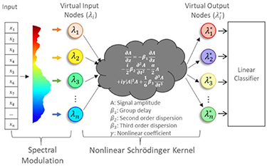
Figure 5. Nonlinear Schrödinger Kernel: samples of input data are first assigned to virtual modes through spectral modulation [28]. The input data is nonlinearly projected to an output representation with a transformation governed by the nonlinear Schrödinger equation (NLSE). © 2022 IEEE. Reprinted, with permission, from [28].
Download figure:
Standard image High-resolution image3.2. Analog computing with metamaterial
Wave propagation in a metamaterial is another emerging field that can be exploited to perform specialized computational tasks such as solving integral equations [29]. Integral equations are ubiquitous in science and engineering and are described by a kernel function which performs a specific transformation of the input function. To create the metamaterial for solving a specific integral equation, an inverse-problem optimization approach was used to identify the structure that exhibits the desired computational kernel.
3.3. Physical emulation of neural networks
Besides analog computing using metamaterials, there is a large body of research centered on emulating neural networks with diffractive optics or optical waveguide circuits with the goal of performing machine learning (ML) at the speed of light. Specific approaches include the use of spatial light modulators for matrix manipulation or using integrated optical circuits involving electrooptic modulators [30, 31].
More recently, the idea of physical neural network is proposed to implement DNNs on various modalities of physical systems such as in mechanics, optics and electronics [32]. Input data and controllable parameters are encoded onto physical quantities such as sound, light and voltage. As they evolve in physical systems, the nonlinear dynamics is a natural form of mathematical transformations as done in neural networks. With a hybrid physical-digital algorithm called physics-aware training, the controllable parameters of the systems can be trained by doing forward pass in the real physical systems and backward pass in digital simulation models. This shows the potential for analog sensors themselves to perform computations directly on signals without using digital processors. It is demonstrated that mechanical, electronic and optics-based physical neural networks can achieve 87%, 93% and 97% test accuracy respectively, on the MNIST dataset.
4. Physics-inspired algorithms
4.1. PhyCV: physics-inspired computer vision library
In addition to physical systems acting as natural computers, principles of physics can be used to design computationally efficient and explainable algorithms for solving problems in multiple domains such as computer vision. PhyCV is a physics-inspired computer vision library [33]. It utilizes algorithms directly derived from the equations of physics governing physical phenomena. Unlike traditional algorithms that are hand-crafted empirical rules, physics-inspired algorithms leverage physical laws of nature as blueprints for crafting algorithms. The current release of PhyCV has two algorithms for computationally efficient edge and texture extraction: Phase-stretch transform (PST) [34] and Phase-Stretch Adaptive Gradient-Field Extractor (PAGE) [35, 36]. They are originated from photonic time stretch [37], a hardware technique for ultrafast and single-shot data acquisition. The algorithms emulate the propagation of light through a 2D physical medium with natural and artificial diffractive properties followed by coherent, i.e. phase detection. PhyCV algorithms do not require training data and may be implemented in real physical devices for fast and efficient analog computation. While the algorithms are deterministic, current implementation is not adaptive therefore the model parameters must be empirically determined.
4.2. Models based on mechanical springs
Another example of a physics inspired algorithm is inspired by a network of mechanical springs to model a complex object consisting of interacting parts. Each part is represented by a node and each edge represents springs with different stiffness parameters to model the interactions. Recent methods have shown how such spring models can be learned in an automated manner from much fewer learning examples than conventional supervised learning methods [38]. This geometric and explainable model (instead of a black-box model) mimics the way the human brain is theorized to represent object categories with a natural model (i.e. elastics) as a basis for the computing.
5. Applications
In the last section, we discuss applications that will be transformed by the emerging techniques of Physics-AI symbiosis including climate modeling, drug discovery and open-source software platforms.
5.1. Climate modeling
Climate change is one of the main challenges facing humanity today. It is of great significance to have accurate and fast climate modeling techniques to predict not only extreme weather, such as hurricanes, but also the impact of climate change. This is challenging since it requires modeling the physics of Earth, including atmosphere, oceans, lands, and human activities etc. Numerical weather prediction attempts to solve the physics equations at large scales given the current conditions. However, the enormous computational complexity only allows low spatial and temporal resolution. It has been shown that deep generative models trained on weather radar data can successfully predict the precipitation for the next 90 min at 5 min and 1 km resolution [39]. Weather forecasting with improved resolution can benefit decision-making in vehicle routing and the planning of public outdoor events. The superior computational efficiency of the neural network approach compared to numerical simulations may lead to a planet-scale model for predicting climate change in the future. Figure 6 shows an example of weather forecast of California Coast.
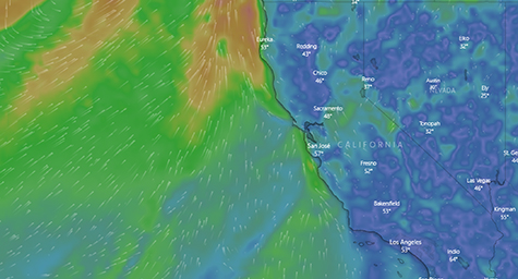
Figure 6. Weather forecast of California coast from the European Centre for Medium-Range Weather Forecasts [40]. Such models are able to predict the weather for approximately 10 days but with limited spatial and temporal resolution and with successively lower accuracy at longer times. Neural networks can potentially lead to more efficient and accurate forecasting results with higher resolution. Reproduced from [40] © OpenStreetMap contributors.
Download figure:
Standard image High-resolution image5.2. Drug discovery
Drug discovery is a large and crucial industry where Physics-AI symbiosis can play a transformative role. A core task in modern drug discovery is to search for molecules with desired properties, e.g. those bind-to and modify the function of a target protein. This requires predicting the interactions between the drug molecule and the target protein. The resulting quantum mechanical calculations require knowledge of the 3D structure of complex proteins. Traditionally, the protein structure is revealed by laborious and time-consuming experimental methods such as x-ray crystallography and cryo-electron microscopy. Recently, AI techniques have shown promise in predicting the 3D structure of proteins purely from their amino acid sequences. AlphaFold [41] achieves accurate prediction results that are competitive to experimental methods and has been applied to predict 98.5% percent of all human proteins. RoseTTAFold [42] achieves similar accuracy with higher computational efficiency. In the meantime, attempts have also been made in controllable protein sequence generation. ProGen adapts the transformer model that is widely used in language modeling to generate desired protein sequences conditioned on taxonomic and keyword tags [43]. These breakthrough AI models can significantly accelerate drug discovery. Figure 7 shows an example of how AI and physics can play the role in the future of drug discovery.

Figure 7. An example of a molecule design pipeline incorporating ML [44]. First, 1000 random molecules are selected from 1 billion candidates. The properties of these molecules are calculated by the free energy perturbation (FEP) software based on physics. The results are used to train a ML model, which in turn is used to rank the original 1 billion candidate molecules. The top 5000 candidates are simulated with the physics models to select the top ten molecules that are then synthesized in the lab and used for downstream testing of their therapeutic efficacy. Reproduced from [44] © Schrodinger.com.
Download figure:
Standard image High-resolution image
5.3. Open-source software and platforms
With emerging techniques in Physics-AI symbiosis, open-source software platforms are becoming increasingly available for developers and researchers. The NVIDIA Modulus is a framework containing physics-ML models [45]. It blends PDEs with AI to design digital twins for complicated nonlinear physical systems. PennyLane is a cross-platform Python library for differentiable programming of quantum computers which could be used for quantum machine learning [46]. Snapchat Lens Studio is an augmented reality application with customization and interactive experiences for graphical editing [47]. With the focus on building industrial-scale digital twins, NVIDIA has introduced the 'Omniverse' [48], an open platform for virtual collaboration and real-time physical simulations in architecture, construction, and manufacturing industries.
6. Conclusion
The power of DNNs stems from having billions or even trillions of free parameters that adapt to data but the training requires massive labeled datasets that are not available in many domains. Also, being a black box, these models lack interpretability and robustness guarantees. Moreover, applications in real-time control such as autonomous vehicles and drones have additional strict requirements for low latency which is challenging to achieve with DNNs. Concurrently, the impressive performance gain in DNNs has come at the expense of exponential growth in network size with the concomitant growth in computational complexity, memory and power consumption [49]. Yet, semiconductor technology is reaching fundamental scaling limits, a trend generally referred to as 'the end of Moore's law'. These trends call for a fresh look into the design of AI systems. Blending physical principles into AI addresses this problem and has already proven to be transformational for both AI and physics.
Broadly speaking, the emerging symbiosis of physics and AI is evolving in three directions. First, AI is providing alternative models to the master equations of physics. Here, laws of physics are blended into the design and training of neural networks, which helps neural networks simulate physics far more efficiently than numerical solvers. In the second direction termed 'physics as a computerʼ, physical systems are utilized to perform specialized computations and therefore reduce the burden on digital processors. Third, physics-inspired algorithms utilize physical phenomena to design efficient and interpretable algorithms. In the meantime, open-source software and platforms for physics-ML and digital twins are emerging, which could potentially revolutionize applications such as climate modeling and drug discovery. While such visionary projects are in their infancy, the symbiosis of these separate fields will surely transform the vector of physics and AI in new and unexpected ways.
Physics-guided neural networks can approximate the equations of physics well but how well can they learn physics? The latest findings suggest that current networks' ability to learn physical intuition is at the level of young children [26]. As of the date of this writing, AI has proven better at learning mathematical relations. For example, AI has been effective in advancing mathematics by learning conjectures [50]. One of the areas to watch in the future is the link between biophysics and machine learning. For example, single-cell bacteria behave as chemotaxis sensors that can classify chemicals [51]. Such works suggest the potential to engineer micro/nano biophysical systems that perform specialized computation tasks in the same spirit as analog computers did in the early days of computing.
Acknowledgment
B J was supported by the Office of Naval Research (ONR) Multi-disciplinary University Research Initiatives (MURI) program on Optical Computing Award No. N00014-14-1-0505. A K was partially supported by ARL W911NF-20-2-0158 under the cooperative A2I2 program, and also partially supported by an Army Young Investigator Award. V R was partially supported by NSF CMMI-2053971.
Data availability statement
No new data were created or analysed in this study.