Graph networks for molecular design

Rocío Mercado; Tobias Rastemo; Edvard Lindelöf; Günter Klambauer; Ola Engkvist; Hongming Chen; Esben Jannik Bjerrum

doi:10.1088/2632-2153/abcf91

1. Introduction

Due to the recent success of deep learning (DL) models across a wide-range of fields, it is often said that we are in the third wave of artificial intelligence (AI) [1]. Some of the most utilized architectures at the forefront of the recent AI boom are recurrent neural networks (RNNs), used to model sequential processes (such as speech), and convolutional neural networks, used in computer vision tasks [2]. More recently, there has been an increase in the use of graph neural networks (GNNs), or more generally, graph networks (GNs) [3], for modeling patterns in graph-structured data. Graphs are widespread mathematical structures that can be used to describe an assortment of relational information, and would seem natural choices for organic chemistry as graphs are natural data structures for describing molecular structures.

The idea of designing novel pharmaceuticals can be boiled down to generating graphs which meet all the criteria of desirable drug-like molecules. This is the guiding principle behind graph-based molecular design. De novo molecular design is the process of designing novel molecules with a specific set of desired pharmacological properties from scratch. This approach is the antithesis of QSAR-based high-throughput screening, where instead the structures are known and their corresponding pharmacological and physical chemical properties are unknown. Deep molecular generative models have emerged as promising methods for exploring the otherwise intractably large chemical space through de novo molecular design [4–13], with the first string-based study emerging in 2016 [14], and the first graph-based studies emerging in 2018 [9, 15].

While string-based methods are surprisingly powerful, graphs are more natural data structures for describing molecules, and have many potential advantages over strings, especially when used with GNs, as GNNs have the ability to learn permutation invariant representations for graphs [16–20]. Additionally, the graph representation can naturally be expanded to include additional descriptors (e.g. spatial coordinates) in applications where more information than simply the identity and connectivity of atoms in a molecule is required (e.g. conformer generation) [21–23]. Finally, GNNs have the potential to learn from fewer examples as they can directly learn the connectivity rules underpinning atoms in molecules, as opposed to, for example, RNNs learning a syntax. All these reasons, supplemented by the relatively more recent development of tools for efficiently working with graphs, make GNNs appealing to study for molecular generation.

Here, a new platform, GraphINVENT, is introduced for training deep generative models directly on the molecular graph representations using GNNs. First, the various elements of GraphINVENT are introduced, with similarities and differences to string-based generative models highlighted along the way. The six different GNNs used in this work are then described in detail in the methods section, together with hyperparameter tuning and training. The Molecular Sets (MOSES) benchmark [24] and other internal evaluation metrics are then used to compare model performance in training speed, reproduction of molecular properties of the training set, and comparison to both string- and graph-based models where metrics have been previously published.

1.1. Graph networks

GNNs are a class of GNs, which have recently emerged as powerful tools for representation learning of graphs [3, 20, 25]. In summary, GNs take graph-structured data as input and output a latent representation for the input graph. This output graph representation is the result of aggregating hidden node states (vectors) obtained in the different propagation blocks of the GN [3, 16, 26]. The learned graph representations are node-order invariant, and a smaller distance between two graph representations implies a greater degree of similarity.

In this work, the representation learning power of GNNs is applied to molecular graph generation. The focus is on GNNs which generalize convolutions to graphs, such as graph convolutional networks (GCNs) and message passing neural networks (MPNNs). The difference between GCNs and MPNNs is that the propagation rules in GCNs can be directly derived from spectral graph theory and approximations thereof, whereas the propagation rules in MPNNs can use 'arbitrary' neighborhood aggregation functions [27]. Being widely referenced throughout this work, the functional form of an MPNN is illustrated in figure 1; MPNNs are discussed in more detail in section 2.1.1.

**Figure 1.** Schematic of a message passing neural network (MPNN), the main class of GNN used in this work. The goal of an MPNN is to learn a graph representation vector, g, via a neighborhood aggregation scheme of node states, $h_i^l$ , and edge states, e_ij.
Download figure:
Standard image High-resolution image

**Figure 1.** Schematic of a message passing neural network (MPNN), the main class of GNN used in this work. The goal of an MPNN is to learn a graph representation vector, g, via a neighborhood aggregation scheme of node states, $h_i^l$ , and edge states, e_ij.
Download figure:
Standard image High-resolution image

Introduced by Scarselli et al in 2008 [25, 28], many GNN variants have since been reported in the literature, the majority applied to molecules only in the past couple of years [16, 20, 27, 29]. The general GNN architecture is L propagation blocks using a non-linear propagation rule,

$\begin{equation} H^{l+1} = f_{{prop}}(H^l, E) \quad \forall \ \ l \in L, \end{equation} \tag{ 1 }$

followed by a readout function. The propagation block can be thought of as a convolution layer. In the expression above, E is the adjacency tensor, and the hidden node states H⁰ are initialized to the node features matrix, X.

The GNN can be used for (local or global) property prediction with an appropriate readout function to obtain the target property $Y = f_{{readout}}(H^L)$ . Often, the goal of a readout function is to calculate a node-order invariant embedding for the molecular graph, g, which can then go on to be used for property prediction tasks.

Different GNNs are distinguished by the specific functions used for f_prop or f_readout.

1.2. Generative models

The last three years has seen a lot of work on DL-based generative models; some of this work will be summarized in the next sections. For more in-depth reviews on generative models, see [30–33].

1.2.1. String-based generative models

Since 2016, extensive work has been done on string-based generative models. Many of these models [4, 34–37] have been benchmarked using the MOSES distribution-based metrics [24], discussed in section 2.4.4. These benchmarked models have been used for comparison with GraphINVENT models.

Many of these string-based generative models borrow methods from natural language processing, such as RNNs, generative adversarial networks (GANs), and autoencoders (AEs), which train on a general set of molecular strings and learn the underlying syntax. A model which has then learned the syntax behind molecular strings in a training set can then be used to generate new molecular strings which sample the same distribution of tokens (e.g. 'C', ' = ', '1') found in the training set. Because these methods are often probabilistic, there is always a chance of sampling a novel permutation of tokens that then leads to new molecular strings not found in the training set, and thus, novel molecules. In drug design, the most common string representation used is SMILES [38]. SMILES and RNNs work incredibly well together for deep molecular generation; for a nice overview of string-based molecular generation, see [39].

1.2.2. Graph-based generative models

The first works on molecular graph generation were published in 2018 [9, 15], and there has since been a surge of graph-based generative models published in the past two years [9–13, 15, 40–60]. Graph-based deep molecular generative models also use a variety of architectures, such as GNNs, AEs, RNNs, and GANs, to learn representations (i.e. vectors) for the different nodes in the graph and/or the graph itself. New molecular graphs can then be generated which sample the prior distribution of nodes and edges. The way in which new nodes and edges are sampled varies greatly between each method; below we detail two.

The methods of Li et al [9, 10] inspired the beginning of this work in late 2018. In these models, new graphs are generated by iteratively adding nodes and edges to incomplete subgraphs; they do this by sampling from learned distributions of possible actions, such that the graph generation process can be seen as a sequence of decisions for each subgraph. Neither of these methods encodes explicit chemical rules into their models, which makes it so impressive that they are able to learn such a large fraction of chemically valid molecules.

We have adopted similar approaches in this work. Two of the local readout functions from [9] have been implemented in GraphINVENT, whereas the action space has been divided similarly to [10]. To build upon that work, many additional GNN blocks were explored in GraphINVENT in combination with a tiered global graph readout function. Moreover, GraphINVENT has then been compared to state-of-the-art (SOTA) methods, something the previous studies did not do.

In [9], the decision space is split into three possible actions for building the graphs: f_addnode, which determines whether to terminate the graph building process or add a new node to the graph; f_addedge, which determines whether to add a new edge to a newly created node; and f_nodes, which determines a score for each node and thus determines which node to build upon next. All of these actions use the learned node and graph embeddings, which are calculated from L stacked GNN blocks. Furthermore, all GNN implementations used can be described using the MPNN framework, discussed in detail in the next section. Many of the message passing and node update functions used in [9] have been implemented in GraphINVENT (e.g. feed-forward neural networks and RNNs), with the exception that GraphINVENT does not use any long short-term memory cells for the message update functions as they were found to be comparable in performance to gated recurrent unit cells. GraphINVENT also uses two of the local readout functions used in [9]: a simple sum and the graph gather function [17], both amply used within the GNN literature.

GraphINVENT differs from [9] in the use of a tiered global readout, as well as in the handling of training data, both to be discussed in detail below. Notably, on-the-fly training data generation was found not to scale to larger training sets (i.e. millions of structures), such that a data preprocessing scheme was adopted in GraphINVENT which would allow it to maintain a relatively low RAM requirement during training. While GraphINVENT has been made publicly available, the authors of Li et al [9] did not publish any code.

In [10], the authors used a similar sequential graph construction approach as discussed above, where sampled actions are iteratively applied to intermediate graphs until the 'terminate' action is sampled. The authors introduce the terminology decoding route to refer to the specific route, r, that is taken to construct a particular graph such that $r = ((\mathcal{G}_0, t_0),(\mathcal{G}_1, t_1),\dots, (\mathcal{G}_N, t_N))$ ; here $\mathcal{G}_n$ is a specific graph state and t_n is an action that takes $\mathcal{G}_n \rightarrow \mathcal{G}_{n+1}$ . We found this terminology very useful when discussing graph generation.

The authors then split their decision space into four possible actions for building subgraphs: initialization, which adds a single node to an empty graph; append, which adds a new node and connects it to an existing node in the graph; connect, which connects the last appended node to another node in the graph; and termination, which ends the graph generation process. The authors deviated from the traditional MPNN framework, and opted instead for the graph convolution architecture published by Wu et al [61]. At each propagation step, each node aggregates information not only from nearest neighbors, but also from remote neighbors. Although a less elegant framework than the one presented above, the authors were able to scale their calculations to molecules containing up to 50 heavy atoms, and even introduced recurrence in one of their models (MolRNN), to much improvement. Our models deviate from theirs in structure both in the GNN blocks and in the global readout blocks, but we have chosen to divide our action space similarly to theirs. The authors of [10] have made their code, which is built using Python 2.7 and scikit-learn, publicly available.

Unfortunately, few of the GNN-based molecular generative models introduced in this section have compared to SOTA methods, such that it is difficult to compare the advantages of each method. This is partly explained due to the relative newness of the field and, until recently, lack of established standards and open-source benchmarking tools; however, following the publication of various open-source benchmarking methods [7, 24, 62], this is likely to change. To the best of our knowledge, one graph-based deep generative model, the JTN-VAE [11], has been benchmarked using the MOSES metrics, making it suitable for comparison with GraphINVENT.

2. Methods

The methods section is organized as follows:

(a)
model architectures;
(b)
model input/output formats;
(c)
training sets;
(d)
workflow;
(e)
evaluation metrics;
(f)
hyperparameter optimization; and
(g)
computational details.

2.1. Model architecture

The generative models in GraphINVENT consist of two segments, which will be referred to as 'blocks':

(a)
a GNN block;
(b)
a global readout block.

These are described in the following subsections. In short, the GNN block takes as input the molecular graph representation, i.e. the adjacency tensor, E, and node features matrix, X, and outputs the transformed node feature vectors, H^L, and the graph embedding, g (figure 2).

**Figure 2.** General schematic of GraphINVENT models. Shown is a single molecule, but in practice both training and generation is done on a mini-batch of graphs.
Download figure:
Standard image High-resolution image

The global readout block then predicts a global property of the graph using H^L and g. Here, the global property one is interested in calculating is the action probability distribution (APD) of each graph, which is a vector containing probabilities for all possible actions for growing a graph; sampling it tells the model how to grow a graph.

As the APD defines all possible actions for growing any subgraph, the APD contains invalid actions from the point of view of a single graph. The model must learn to assign zero probability to invalid actions for a given input graph.

2.1.1. The GNN block

Six unique GNN blocks were constructed in GraphINVENT. Each GNN block is a different MPNN [16]. These are:

(a)
MNN—message neural network.
(b)
GGNN—gated-graph neural network [17, 63].
(c)
S2V—set2vec [63, 64].
(d)
AttGGNN—GGNN with attention [63].
(e)
AttS2V—S2V with attention [63].
(f)
EMN—edge memory network [63, 65].

The MNN has not been investigated before for molecular tasks. The names from the list above are used both here and in the code. This is emphasized as some of the above networks have inconsistent names in the literature. The names of the GNN blocks are also used to refer to the models in GraphINVENT, as the GNN block is what distinguishes them.

Many of these GNNs have been previously explored for property prediction tasks [16, 19, 65–67] and found to be comparable to SOTA methods, but they have not been tested in architectures for generative tasks.

The first three MPNN implementations—MNN, GGNN, and S2V—can be represented using the following functional form.

(1) A message passing phase, consisting of l ∈ L message passing blocks:

$\begin{align*} &m_i^{l+1} = \sum_{v_j \in \mathcal{N}(v_i)} M_l \left(h_i^l, h_j^l, e_{ij}\right) \\ &h_i^{l+1} = U_l \left(h_i^l, m_i^{l+1}\right), \end{align*}$

where m_i and h_i are the incoming messages and hidden states of node v_i, $\mathcal{N}(v_i)$ is the set of v_i's nearest neighbors, and e_ij is the edge feature vector for the edge connecting v_i and v_j. M_l and U_l are the message passing and node update functions, respectively. The message passing phase is followed by the following.

(2) A graph readout phase:

$\begin{equation*} g = R(H^L, H^0), \end{equation*}$

where g is the final graph embedding. The graph readout, R, is an aggregation function that collects the initial and final node states, transforms them, and returns a single graph embedding.

The fourth and fifth implementations—AttGGNN and AttS2V—can almost be represented using the same functional form, but with a slight modification to the message passing phase:

$\begin{align*} &m_i^{l+1, ^{\prime}} = \sum_{v_j \in \mathcal{N}(v_i)} w_{ij}^l \odot M_l \left(h_i^l, h_j^l, e_{ij}\right) \\ &h_i^{l+1} = U_l \left(h_i^l, m_i^{l+1, ^{\prime}}\right), \end{align*}$

where $\odot$ is the element-wise multiplication operator, and

$\begin{equation*} w_{ij}^l = \texttt{SOFTMAX}(f(h_j^l), \mathcal{N}(v_i)). \end{equation*}$

The second argument above indicates the set over which the softmax is computed (if the second argument is omitted, then the softmax is applied over the dimension of the input vector). For example, using $\mathcal{N}(v_i)$ above ensures that $\sum_{v_j \in \mathcal{N}(v_i)} w_{ij}^l = (1,\ldots,1)$ . This is a form of attention [68].

Finally, the sixth implementation (EMN), can also be described using the attention description above; however, instead of having hidden states on the nodes, hidden states are on the edges, and messages are passed between edges, such that the role of the edges and nodes is flipped.

The precise functions used for M_t, U_t, and R in each of the six models discussed herein can be found in appendix C.

2.1.2. Global readout block

The GNN block is followed by a global readout block. The global readout block uses both the node- and graph-level information to predict the APD. Many different global readout block architectures were tested before selecting the one presented here, and are described elsewhere [69].

The global readout block has a tiered multi-layer perceptron (MLP) structure, where the first two MLPs generate a preliminary $f_{add}^{\,^{\prime}}$ and $f_{conn}^{\,^{\prime}}$ (see section 2.2.2), which are then concatenated with the graph embedding g. This concatenated tensor is input to the second block of MLPs, and their output concatenated and normalized to return the APD. Note that f_term only depends on g.

$\begin{align*} f_{add}^{\,^{\prime}} & = \texttt{MLP}^{add, 1} \left(H^L \right) \\ f_{conn}^{\,^{\prime}} & = \texttt{MLP}^{conn, 1} \left(H^L \right) \\ f_{add} & = \texttt{MLP}^{add, 2} \left( [ f_{add}^{\,^{\prime}}, g ] \right) \\ f_{conn} & = \texttt{MLP}^{conn, 2} \left( [ f_{conn}^{\,^{\prime}}, g ] \right) \\ f_{term} & = \texttt{MLP}^{term, 2} \left( g \right) \\ APD & = \texttt{SOFTMAX} \left(\left[ f_{add}, f_{conn}, f_{term} \right] \right). \end{align*}$

2.2. Model input and output

2.2.1. Model input

The input to all GraphINVENT models is the molecular graph representation. All the graphs in this work are represented by the following two tensors:

(a)
node features matrix, $X \in \{0, 1\}^{|\mathcal{V}^{\textrm{max}}| \times C}$
(b)
adjacency tensor, $E \in \{0, 1\}^{|\mathcal{V}^{\textrm{max}}| \times |\mathcal{V}^{\textrm{max}}| \times |\mathcal{B}|}$ .

$|\mathcal{V}^{\textrm{max}}|$ and $|\mathcal{E}^{\textrm{max}}|$ are the number of nodes and edges, respectively, in the largest graph in the dataset. For all graphs, X and E are padded to the size of the largest graph in the dataset. For a detailed example, see appendix D.

Above, C is a constant which denotes the size of the node features; it is the sum of the number of one-hot encoded features per node, $C = |\mathcal{A}| + |\mathcal{F}| + |\mathcal{H}| + |\mathcal{C}|$ (table 2). The size of the edge features is the number of one-hot encoded features per edge, $|\mathcal{B}|$ (table 3).

Table 1. Datasets used in this work.

Dataset	Size^a	Size^b	\| $\mathcal{V}^{\textrm{max}}$ \|	Atom types	Formal charges
GDB-13 1K rand	1K, 1K, 1K	12K, 12K, 12K	13	{C, N, O, S, Cl}	{−1, 0, +1}
GDB-13 1K canon	1K, 1K, 1K	12K, 11K, 11K	13	{C, N, O, S, Cl}	{−1, 0, +1}
MOSES rand	1.5M, 176K, 10K	33M, 3.8M, 210K	27	{C, N, O, F, S, Cl, Br}	{0}
MOSES canon	1.5M, 176K, 10K	26M, 3.3M, 192K	27	{C, N, O, F, S, Cl, Br}	{0}
MOSES arom	1.5M, 176K, 10K	40M, 4.4M, 247K	27	{C, N, O, F, S, Cl, Br}	{0}

Here, the size of each split (train, test, val) is the number of graphs ^a before and ^b after preprocessing, rounded. 1K = 1000; 1M = 1 000 000.

Table 2. Node features used in graph representations in this work. The specific elements in each set are user-defined and depend on the dataset used. Asterisks (*) denote optional features.

Node feature	Set label	Example elements
Atom Type	$\mathcal{A}$	{C, N, O, S, Cl}
Formal Charge	$\mathcal{F}$	{−1, 0, +1}
Implicit Hs*	$\mathcal{H}$	{0, 1, 2, 3}
Chirality*	$\mathcal{C}$	{None, S, R}

Table 3. Edge features used in graph representations in this work. The asterisk (*) denotes an optional element in the bond set.

Edge feature	Set label	Elements
Bond Type	$\mathcal{B}$	{Single, Double,
		Triple, Aromatic*}

2.2.2. Model output

The learned output for all of the models is the APD, which specifies how to grow the input subgraphs. The APD is made up of three components: f_add, f_conn, and f_term, similar to previous work [10].

f_add contains probabilities for adding a new node to the graph. f_conn contains probabilities for connecting the last appended node in the graph to another existing node in the graph. f_term is the probability of terminating the graph.

The shapes of the three (unflattened) APD components are described in tables 4–6. The APD is a vector property which contains the probabilities of all possible actions for growing an input subgraph; as it is a vector property, f_add and f_conn are flattened in the APD. The APD for each graph sums to 1.

Table 4. f_add tensor shape for a mini-batch of graphs. Optional dimensions are indicated by an asterisk (*). Any nonzero term in f_add means there is a possibility of appending a new node to the graph with the features indicated by dims 2–5 using the bond type indicated by dimension 6. The new node will be appended to the node denoted by dimension 1. γ is the mini-batch size.

Dim	Property	Size
0	Subgraph index	γ
1	Node to connect to	$\|\mathcal{V}^{\textrm{max}}\|$
2	New atom type	$\|\mathcal{A}\|$
3	New formal charge	$\|\mathcal{F}\|$
4*	New implicit Hs	$\|\mathcal{H}\|$
5*	New chirality	$\|\mathcal{C}\|$
6	New bond type	$\|\mathcal{B}\|$

Table 5. f_conn tensor shape for a mini-batch of graphs. Any nonzero term in f_conn means there is a possibility of appending the last appended node to the node denoted by dimension 1, with the bond type indicated by dimension 2. γ is the mini-batch size.

Dim	Property	Size
0	Subgraph index	γ
1	Node to connect to	$\|\mathcal{V}^{\textrm{max}}\|$
2	New bond type	$\|\mathcal{B}\|$

Table 6. f_term tensor shape for a mini-batch of graphs. Any nonzero term in f_term means that there is a possibility of terminating that graph's generation. γ is the mini-batch size.

Dim	Property	Size
0	Subgraph index	γ

2.2.3. The graph decoding route

The APDs are computed for all graphs in the training set during preprocessing, and are the target vectors to learn during training. The APDs can be derived from the graph decoding route as outlined below.

Li et al [10] introduced the concept of a graph decoding route in their work, using it to refer to the specific route, r, that has been taken to construct a particular graph. GraphINVENT uses a similar concept. For each graph in the training data, $r = ((\mathcal{G}_0, APD_0),(\mathcal{G}_1, APD_1),\dots, (\mathcal{G}_N, APD_N))$ is computed. Here, APD_n describes how to get from $\mathcal{G}_n$ to $\mathcal{G}_{n+1}$ , $\mathcal{G}_0$ is an empty graph, $\mathcal{G}_N$ is the final graph, and N is the total number of construction actions. $\mathcal{G}_{1 \ldots N-1}$ are the intermediate sized graphs. APD_N encodes the final 'terminate' action.

Which subgraphs are found in r is determined by how the graph is traversed; this is detailed in section 2.4.1 below.

2.3. Training sets

Datasets used in this work are listed in table 1. The GDB-13 1K subsets each consist of 1000 randomly selected structures from the full GDB-13 dataset [70]. The GDB-13 dataset is made up of small organic molecules generated in silico so as to enumerate the chemical space of up to 13 heavy atoms (with a few additional constraints). This dataset was used for quick hyperparameter optimization runs.

The MOSES datasets were used for evaluating GraphINVENT models and were downloaded from the MOSES GitHub [71]. The MOSES dataset is a subset of the ZINC dataset [72], and consists of slightly larger commercially available organic molecules, curated for virtual screenings.

Subsets of MOSES were also used to test the effect of dataset size on learning; these subsets were obtained by randomly sampling 10% and 1% of structures from the full MOSES dataset.

2.4. Workflow

The workflow can be split up into four general phases:

(a)
preprocessing;
(b)
training;
(c)
generation; and
(d)
benchmarking

Each of these phases is detailed below. With the exception of preprocessing, all the workflows were non-trivially parallelized for faster performance on a GPU.

2.4.1. Preprocessing

In order for a model to learn to build molecular graphs, the training set molecules must be preprocessed in a way that the model can learn how to reconstruct them. The model cannot simply be fed the final molecule, but also information on how to build the molecule from an empty graph in a step-by-step fashion.

Preprocessing the training data is in essence a graph traversal problem. To create the training data, all molecules in the training set are fragmented step-wise (Algorithm 1 in appendix E), so as to obtain each molecule's decoding route, r. Each time a graph $\mathcal{G}_n$ is fragmented into $\mathcal{G}_{n-1}$ , the corresponding APD_n − 1 is computed for $\mathcal{G}_{n-1}$ ; APD_n − 1 contains the information needed to reconstruct $\mathcal{G}_n$ .

The order of the node/edge removal is determined by reversing a breadth-first search (BFS) (Algorithm 2 in appendix E), modified to ensure that disconnected fragments in the graph are never created after removing any edge.

Starting with a molecular graph $\mathcal{G}_N$ from the training set, r is calculated via the following steps:

(a)
Assign a rank to each node v_i in $\mathcal{G}_N$ . This rank can be either (a) random or (b) canonical⁵ .
(b)
Traverse graph using modified BFS algorithm. Let $\mathcal{O}_{BFS}(\mathcal{V}_N)$ be the graph traversal node order.
(c)
Using $\mathcal{O}_{BFS}$ , deconstruct graph step-by-step until empty graph, $\mathcal{G}_0$ , is reached, to obtain r.
(d)
Repeat for all graphs in the mini-batch.

The deconstruction algorithm is illustrated in figure 3.

**Figure 3.** Graph deconstruction used by GraphINVENT during training data preprocessing. The numbers on the nodes correspond to $\mathcal{O}_{BFS}$ . The last node traversed using the mod-BFS algorithm will be the first node to be removed (node 4), followed by the second-to-last node traversed (node 3). However, as node 3 has two edges, one edge must first be removed; in the next deconstruction step, node 3 and the remaining edge are removed together. This process is repeated until there are no nodes remaining in the graph.
Download figure:
Standard image High-resolution image

2.4.2. Training

Training is done in mini-batches. The training loss in the models is the Kullback–Leibler divergence between the target APD and predicted APD. All models are trained using the Adam optimizer using the default PyTorch parameters (except for weight decay in specified cases).

During training runs, the models are evaluated by sampling n_samples graphs every fixed number of epochs. The generated graphs are used to calculate the evaluation metrics detailed in section 2.4.4. The model state is saved after every evaluation epoch.

2.4.3. Generation

GraphINVENT models receive graphs as input and output APDs, from which possible actions can be sampled and applied to the graphs. As detailed above in section 2.2.2, the three possible actions are

adding a new node to the graph;
connecting the last appended node to another node in the graph; and
terminating the graph construction.

The specific details of each action (e.g. what type of atom to add) are encoded as nonzero elements in the APD. The graph generation scheme is illustrated in figure 4.

**Figure 4.** Graph generation scheme in GraphINVENT. Upon seeing a graph, a trained model predicts an APD for the input graph. An action is then sampled from the APD and applied to the graph to generate the next graph in the sequence. The process is repeated until the 'terminate' action is sampled.
Download figure:
Standard image High-resolution image

Invalid actions are not masked during graph generation, as well-trained models will seldom sample these and it is desirable to avoid hard-coding any rules into the models. Furthermore, invalid actions are not masked so as to avoid artificially inflating the quality of generated molecules.

As such, in addition to sampling the 'terminate' action, the generation process is terminated for a graph if an invalid action is sampled for it. There are three invalid actions which can occur during generation. These are attempts to:

(a)
add a node to a non-existing node in a graph⁶ ,
(b)
connect a pair of already-connected nodes; or
(c)
add a node to a graph already having the maximum number of nodes.

None of these invalid actions are chemistry related, but rather graph related.

If hydrogens are ignored during training data preprocessing, they are also ignored during generation. In such cases, hydrogens are added to the generated graphs using RDKit [73] based on the valency of each atom.

Deciding at which point to stop training a generative model and use it for generating new and interesting structures is a task-dependent question. In this study, training was stopped when the training loss of a model had converged to within three significant figures. Early stopping criteria were also investigated, but found not to work as well as simply training until convergence [69].

2.4.4. Benchmarking

The MOSES benchmark consists of distribution-based metrics for generative models and uses subsets of ZINC [72] for the training and hold-out test sets. MOSES benchmarks were run using the code available at [71]. 30 000 samples were used for evaluating each GNN-based model.

The benchmarking metrics computed by MOSES are as follows:

Fréchet ChemNet Distance (FCD) : difference in distributions of last layer activations in ChemNet [74] between generated and test sets.
Nearest neighbor similarity (SNN) : average similarity of generated molecules to nearest molecule from test set(s).
Fragment similarity (Frag) : cosine distances between histograms of fragment occurrences corresponding to the generated and test set(s).
Scaffold similarity (Scaff) : cosine distances between histograms of scaffold occurrences corresponding to the generated and test set(s).
Internal diversity (IntDiv1 & IntDiv2) : accesses chemical diversity within set of generated molecules (digit indicates different powers of the Tanimoto similarity).
Filters : fraction of molecules passing various chemistry filters.

Furthermore, the FCDs for the following molecular properties are calculated between the generated and test sets: lipophilicity (logP), Synthetic Accessibility score (SA), Quantitative Estimation of Drug-likeness (QED), Natural Product-likeness score (NP), and molecular weight (MW). All of the above metrics are calculated for two test sets: a holdout test set (Test) and a scaffold-only test set (TestSF).

2.5. Evaluation metrics

To evaluate the performance of GraphINVENT models, the following metrics were calculated for each generated set:

PV : Percent valid molecules.
PU : Percent unique molecules.
PPT : Percent molecules that were 'properly terminated' via sampling of a terminate action (as opposed to sampling of an invalid action).
PVPT : Percent of valid molecules in the set of PPT molecules.
$\mathcal{V}_{\text{av}}$ : Average number of nodes per graph.
$\mathcal{E}_{\text{av}}$ : Average number of edges per node.
UC-JSD : The uniformity-completeness Jensen–Shannon Divergence introduced in [7]. This is a similarity measure for the distributions of negative log-likelihood (NLL) per sampled action for the training, validation, and generation sets.

When reporting PU, it is necessary to also report the size of the generated set because as n_samples $\rightarrow \infty$ , PU $\rightarrow 0$ .

For computing the PV and PU, the graphs are first converted to canonical SMILES as it is easier to do string comparison than graph comparison. To do this, graphs are first converted to Mol objects, then converted to SMILES. If the rdkit.Chem.MolToSmiles() function raises an exception, it is caught and the corresponding graph is flagged as invalid.

2.6. Hyperparameter optimization (HO)

HO is crucial for the models presented here. Without suitable hyperparameters, the models will not train well and the molecules generated will be largely invalid.

An initial HO was first performed using GDB-13 1K, as models train in a couple minutes on GDB-13 1K and thus a wide range of hyperparameters could be investigated. The best hyperparameters were then used as a starting point for HO on the significantly larger MOSES dataset. The HO strategy is discussed further in appendix F.

2.7. Computational details

All the software was written in Python 3.6.8 and is available at https://github.com/MolecularAI/GraphINVENT. The models were written using PyTorch 1.3 [75], cudatoolkit 10.0.130, NumPy 1.17.3, tensorboard 2.1.0, and RDKit 2019.03.4.0. The Conda environment specifications used for all calculations in this work can be found in the GitHub repository. All plots were made using matplotlib 3.1.1. The GPU hardware used to train the models were NVIDIA Tesla K80 and Volta V100 16 GB VRAM cards using CUDA 10.0 and driver version 418.87.01, with development on a machine with an NVIDIA RTX-2080 Ti card using CUDA 10.1 and driver version 430.50.

3. Results

3.1. Model evaluation

The performance of all the models using the GDB-13 1K and MOSES datasets is detailed in appendix G. Using the evaluation metrics alone, all GraphINVENT models actually perform decently well, with MNN performing slightly better and AttS2V performing slightly worse on both datasets. The top three models were: MNN, GGNN, and S2V. The models all averaged around 94% PV and successfully modeled the GDB-13 1K prior at Epoch 400. As this dataset has only 1K structures, the low PU for these models (57%–78%) is not concerning.

On the MOSES dataset, all top three models averaged around 95% PV and 99.8% PU while successfully modeling the prior at Epoch 30. While it was not possible to select the best model from the evaluation metrics alone, the MOSES benchmarks (discussed below) revealed the GGNN model to have a slight advantage over the MNN and S2V models for molecular generation tasks. The performance of the best GGNN models trained on the MOSES dataset is highlighted in table 7. All GGNN models achieve PV $\gt$ 90 and PU $\gt$ 99 (n_samples = 30 000).

Table 7. Performance of the best GGNN models using the MOSES datasets; r = random, c = canonical, +w = with weight decay, and a = aromatic. Bold values indicate the best value for each field.

Model	rGGNN	cGGNN	rGGNN+w	cGGNN+w	aGGNN	Target
sampling epoch	40	40	50	50	40	—
deconstruction	random	canon	random	canon	canon	—
use_aromatic	False	False	False	False	True	—
weight_decay	0.0	0.0	0.001	0.001	0.0	—
PV	95.1	96.4	77.8	89.4	95.5	100
PPT	97.1	98.0	83.2	89.4	98.8	100
PVPT	95.1	96.9	76.9	87.4	95.3	100
PU^a	99.1	99.5	94.2	94.3	97.9	100
$\mathcal{V}_{\text{av}}$	22.073	21.877	21.194	20.063	22.082	21.672
$\mathcal{E}_{\text{av}}$	2.149	2.138	2.183	2.132	2.156	2.146

^a n_samples = 30 000.

3.1.1. Canonical deconstruction path

The node ranking used to traverse the graphs and process training data has an effect on how the models learn.

When using a canonical deconstruction path⁷ to preprocess training data (appendix H.3) instead of a random deconstruction path (appendix G.1), an improvement in both the PV and PU was observed in the structures sampled when using GDB-13 1K (c.a. +1% increase in PV, and +5% increase in PU).

Furthermore, canonical deconstruction with dropout leads to a slight negative to negligible effect on the PV and PU for most of the models studied compared to using randomly deconstructed training data with dropout (appendix H.1). Weight decay, on the other hand, has a positive effect on the PU while only marginally decreasing the PV for all models (appendix H.2). Using canonicalization with weight decay is thus a viable way of increasing the uniqueness of the generated structures.

Similarly, using a canonical deconstruction path for the MOSES dataset leads to models with slightly higher PV and PU (table 7). As such, canonical deconstruction is recommended for GraphINVENT models.

3.1.2. Effect of dataset size

The effect of training set size was investigated using the best model, cGGNN, by training on both 10% and 1% random MOSES subsets. Detailed results are available in appendix G.2.0.1.

With 10% of the dataset, the model still performs well: >90% PV and >99% PU (n_samples = 30 000). However, achieving a comparable PV using only 1% of the dataset requires heavy overfitting of the model; at Epoch 100 the models achieve 92% PV, but the PU drops to 70%. These results suggest that the ideal dataset for GNN-based molecular generation contains at least 100 000 molecules, although the models can still learn from less data.

3.2. Benchmarking

3.2.1. Distribution-based benchmarks

GraphINVENT models were benchmarked using the MOSES distribution-based benchmarks. Results are summarized in tables 9–11 for all models at Epoch 10. This epoch was chosen for comparison as it is achievable by all models, with the limiting model being the EMN (10 epochs = 23 GPU days). The best GGNN models (table 7) were also benchmarked at their respective best epochs.

Table 8. Run time for GraphINVENT models. All time averages are calculated using the GDB-13 1K random set.

Model	Prep. ^a	Train. ^b	Gen. ^c	Bench. ^d
MNN	29	345 (2.8)	1311	1.5
GGNN	—	287 (3.4)	1488	—
S2V	—	228 (4.3)	1068	—
AttGGNN	—	80 (12.2)	161	—
AttS2V	—	75 (13.0)	158	—
EMN	—	33 (29.5)	43	—

^aMolecules per second (model-independent).^bMolecules per second (in parentheses: seconds per epoch).^cMolecules per second.^dHours (model-independent).

Table 9. MOSES benchmarks using the holdout test set. The bottom-most set of models are introduced in GraphINVENT; r = random, c = canonical, +w = with weight decay, a = aromatic, and (N) = sampled at epoch N. Results continued in table 10. Bold values indicate the best value for each field, considering previously benchmarked models and the models introduced here-in separately.

Model	Valid	Uni. 1k	Uni. 10k	FCD ( $\downarrow$ )	SNN ( $\uparrow$ )	Frag ( $\uparrow$ )	Scaff ( $\uparrow$ )	IntDiv ( $\uparrow$ )	IntDiv2 ( $\uparrow$ )
Train	1.000	1.000	1.000	0.008	0.642	1.000	0.991	0.857	0.851
AAE	0.937	1.000	0.997	0.556	0.608	0.991	0.902	0.856	0.85
CharRNN	0.975	1.000	0.999	0.073	0.601	1.000	0.924	0.856	0.85
VAE	0.977	1.000	0.998	0.099	0.626	0.999	0.939	0.856	0.85
LatentGAN	0.897	1.000	0.997	0.296	0.538	0.999	0.886	0.857	0.85
JTN-VAE	1.000	1.000	0.999	0.422	0.556	0.996	0.892	0.851	0.845
rMNN (10)	0.946	1.000	0.999	2.199	0.498	0.992	0.827	0.861	0.855
rGGNN (10)	0.925	1.000	0.999	1.872	0.502	0.982	0.732	0.864	0.858
rAttGGNN (10)	0.891	0.997	0.995	2.127	0.468	0.988	0.752	0.872	0.866
rS2V (10)	0.931	0.999	0.999	3.264	0.467	0.985	0.835	0.876	0.869
rAttS2V (10)	0.769	0.987	0.989	2.567	0.484	0.986	0.830	0.870	0.863
rEMN (10)	0.924	0.999	0.998	0.870	0.533	0.993	0.881	0.861	0.855
rGGNN (40)	0.951	0.999	0.996	2.783	0.516	0.966	0.592	0.858	0.852
cGGNN (40)	0.964	1.000	0.998	0.682	0.569	0.986	0.885	0.857	0.851
rGGNN+w (50)	0.778	0.969	0.967	6.577	0.386	0.980	0.529	0.887	0.877
cGGNN+w (50)	0.894	0.958	0.962	3.563	0.493	0.958	0.663	0.867	0.855
aGGNN (40)	0.955	0.965	0.942	3.460	0.497	0.977	0.382	0.873	0.856

Highlighted row = best model introduced in this work.

Table 10. Table 9 cont. MOSES benchmarks for the various models using the holdout scaffold set, plus Filters scores. Bold values indicate the best value for each field, considering previously benchmarked models and the models introduced here-in separately.

Model	FCD ( $\downarrow$ )	SNN ( $\uparrow$ )	Frag ( $\uparrow$ )	Scaff ( $\uparrow$ )	Filters ( $\uparrow$ )
Train	0.476	0.586	0.999	1.000	1.000
AAE	1.057	0.568	0.99	0.079	0.996
CharRNN	0.52	0.565	0.998	0.11	0.994
VAE	0.567	0.578	0.998	0.059	0.997
LatentGAN	0.824	0.514	0.998	0.1	0.973
JTN-VAE	0.996	0.527	0.995	0.1	0.978
rMNN (10)	2.914	0.477	0.987	0.082	0.838
rGGNN (10)	2.292	0.486	0.984	0.134	0.884
rAttGGNN (10)	2.747	0.451	0.987	0.160	0.857
rS2V (10)	4.247	0.443	0.982	0.113	0.835
rAttS2V (10)	3.231	0.462	0.982	0.112	0.829
rEMN (10)	1.436	0.508	0.992	0.151	0.939
rGGNN (40)	3.101	0.499	0.969	0.137	0.919
cGGNN (40)	1.223	0.539	0.986	0.127	0.950
rGGNN+w (50)	6.991	0.378	0.980	0.103	0.722
cGGNN+w (50)	4.265	0.473	0.953	0.129	0.871
aGGNN (40)	3.862	0.478	0.980	0.117	0.897

Table 11. FCD between distributions of the generated and test set(s) for the following properties: logP (lipophilicity), SA (Synthetic Accessibility), NP (Natural Product-likeness), QED (Quantitative Estimation of Drug-likeness), and MW (molecular weight). Bold values indicate the best value for each field, considering previously benchmarked models and the models introduced here-in separately.

	logP	$\times$ e⁻¹	SA		QED	$\times$ e⁻³	NP	$\times$ e ⁻¹	MW
Model	Test	TestSF	Test	TestSF	Test	TestSF	Test	TestSF	Test	TestSF
AAE	0.054	—	0.0048	—	0.043	—	—	—	96	—
CharRNN	0.039	—	0.0004	—	0.0053	—	—	—	5.3	—
VAE	0.0058	—	0.00019	—	0.00025	—	—	—	1.1	—
LatentGAN	0.061	—	0.01	—	0.074	—	—	—	46	—
JTN-VAE	0.055	—	0.016	—	0.012	—	—	—	0.54	—
rMNN (10)	0.116	0.068	0.358	0.360	0.652	0.670	1.653	1.867	54.7	68.5
rGGNN (10)	0.092	0.212	0.304	0.302	0.077	0.085	0.716	0.858	90.8	95.5
rAttGGNN (10)	0.297	0.558	0.560	0.556	0.587	0.607	2.331	2.583	219.3	259.9
rS2V (10)	0.062	0.121	0.458	0.457	0.430	0.449	3.833	4.145	331.6	428.9
rAttS2V (10)	0.199	0.115	0.486	0.487	3.711	3.764	2.350	2.607	523.2	575.8
rEMN (10)	0.320	0.147	0.060	0.061	0.395	0.410	0.3205	0.4193	91.822	128.47
rGGNN (40)	0.068	0.212	0.279	0.275	0.065	0.076	1.659	1.853	37.556	39.635
cGGNN (40)	0.067	0.048	0.045	0.047	0.252	0.269	0.122	0.188	16.1	14.8
rGGNN+w (50)	1.892	2.475	1.925	1.916	6.385	6.455	7.841	8.255	1840.4	1952.1
cGGNN+w (50)	0.549	0.854	0.670	0.673	3.387	3.425	1.414	1.616	1744.1	1885.2
aGGNN (40)	2.954	3.7304	1.560	1.560	1.472	1.503	2.621	2.884	453.69	508.18

While all the models introduced in this work perform reasonably well for all MOSES benchmarks, the GGNN models are consistently the best, performing on par with previously published models. The cGGNN performs the best.

3.2.2. Best model—cGGNN

Using the MOSES dataset, both the rGGNN and cGGNN peaked at Epoch 40. At this epoch, generated structures are most similar to the test set structures based on the FCD distances (table 11) and give the best results across the various MOSES benchmarks (tables 9 and 10). Nonetheless, the cGGNN model has a slight edge on most MOSES metrics. Examples of generated molecules using some of the best models are shown in appendix I.

Based exclusively on the MOSES metrics at Epoch 10, the rEMN model could be the best model. EMN models train significantly slower than the other GraphINVENT models, however, and are impractical for training on MOSES.

3.3. Hyperparameter optimization (HO)

3.3.1. Transferability of hyperparameters

The best hyperparameters for the GDB-13 1K set were used as a starting point for the MOSES dataset. These worked well except for the learning rate decay scheme. As the MOSES dataset is significantly larger (table 1), keeping the batch size fixed (1000) means many more mini-batches need to be processed in MOSES. As such, the learning rate decay scheme was adjusted by increasing the learning rate decay interval (lrdi) to 10 000 for the larger dataset. Further optimization was not performed.

3.3.2. Optimizing the best model—the GGNN

The effect of various (optional) parameters on performance was investigated for the best model, the GGNN. These variants of the GGNN were: aromatic bonds (aGGNN), canonicalization (cGGNN), randomization (rGGNN), training set size, and regularization(GGNN+w). Results are shown in tables 7, 9, 10, and 11.

The best models were rGGNN and cGGNN, with the canonical model performing better than the random model. Adding weight decay to these models worsened their performance across all MOSES metrics—both PV and PU dropped significantly. Even with low weight decay values, the models could not reach a low enough loss. Models also took longer to train.

Including aromatic bond representations noticeably (although not prohibitively) slowed down the training time of GraphINVENT models as it led to more graphs in the preprocessed training data. This is a direct result of having the additional bond type available, which increases the available set of graph matrix representations. The aGGNN model can generate graphs resembling the prior with high PV and PU, but does not perform as well as the cGGNN model on the MOSES benchmarks. However, the aGGNN is on par with the other GGNN models.

3.4. Computational resource requirements

Run times for the three different job types in this work are listed in table 8. Care was taken to obtain all run time benchmarks using the same dataset (GDB-13 1K), hyperparameters (table G6), and GPU card (NVIDIA RTX-2080 Ti).

All jobs are parameter and dataset dependent. It takes a lot longer to process larger molecules with more atom and edge types. As such, while the GDB-13 1K rand dataset takes 2 min to preprocess in its entirety, the MOSES rand dataset takes c.a. 11 CPU days, and the MOSES canon dataset c.a. 5.7 CPU days. Using canonicalization generally cuts the preprocessing speed in half as there are more repeat graphs.

The MNN, GGNN, and S2V models not only train faster, but also generate structures faster, than the three Attention models. This gives them a significant practical advantage. The GPU memory requirement of Training and Generation jobs was generally <10 GB.

The benchmarking time was calculated using 30 000 samples and running MOSES benchmarking jobs for both the Test and Scaffold benchmarks. The GPU memory requirement for Benchmarking jobs using MOSES was 33 GB.

4. Discussion

4.1. Advantages of GraphINVENT models

Good performance against SOTA methods. The GNN-based generative models introduced here perform on par with SOTA benchmarked models on most metrics (FCD, SNN, Frag, Scaf, logP, MW), even performing better than most SOTA models on certain metrics (IntDiv).

Robustness. It has been previously reported that generative models using GNNs can be unstable, converging to different solutions on different runs using the same set of hyperparameters [9]. However, once an adequate set of hyperparameters was identified, these GNN-based models were actually highly robust and stable during training.

High diversity of generated structures. As mentioned previously, all GNN-based models introduced here can generate highly diverse structures when trained on the MOSES dataset. This is evidenced by the high PU and IntDiv scores. This could be highly advantageous for tasks such as library design.

Quick training. Compared to the training time for published graph-based generative models, the MNN, GGNN, and S2V models reported here are very quick to train. In one day of compute time on a single GPU, these models can reach 10+ training epochs on the MOSES dataset. As such, a model can be fully trained in a matter of a few days. Not all datasets of interest are as large as the MOSES dataset, and as such potential users could expect even faster training times. This compares favorably to other published models, such as the JTN-VAE and hgraph2graph [58] models, which are reportedly slow to train (although they give good performance). Nonetheless, there are no current studies comparing the training time on equivalent hardware.

Convergence in relatively few epochs. Compared to string-based models such as CharRNN [76] and REINVENT [7], GNN-based models reach convergence on relatively few epochs (i.e. tens versus hundreds for the MOSES dataset). This could be considered an advantage, as it means GNN-based models do not need to see the structures as often as do RNN-based models, and suggests GNNs could be more efficient at learning the chemistry of training set molecules.

Training on small datasets. GraphINVENT models perform well even with only 1% of the MOSES dataset. As such, reducing the size of the dataset is something that can easily be done without worrying about drastic changes in performance. Furthermore, GraphINVENT models are even able to learn complex chemical rules with high fidelity from only 1000 structures (GDB-13 1K).

Flexible input representation. It is straightforward to expand the graph matrix representation to accommodate additional features. This is done by appending new elements to the node feature vectors x_i and edge feature vectors e_ij of a graph. Examples of features researchers might be interested in include: valencies, atomic radii, quantum mechanical properties, and spatial information (3D coordinates, bond lengths, bond angles, and torsional angles).

4.2. Disadvantages of GraphINVENT models

Relatively low PV. Many SOTA string-based models have PVs above 95%, and some even 100%. By comparison, the best GNN-based generative model presented here reaches a relatively lower 96% PV. Exploring how to increase the PV further without affecting the high PU of these models is a subject of future work.

As a way of increasing the PV, adding a mask that blocks invalid actions from being sampled during the generation phase was considered. The mask, however, was ultimately removed, as it was the equivalent of simply generating more structures and then removing the invalid graphs. This is because using a mask slows down the sampling phase. Not using a mask has the additional advantage that different GraphINVENT models can still be compared on the basis of PV—otherwise all decent models would trivially reach ~100% valid structures.

Hyperparameter optimization is challenging. As with any DL model, HO is crucial for successfully training a GNN-based model. However, this proved to be more challenging than expected in GraphINVENT. Although published hyperparameters for similar MPNN implementations were used as an initial guideline [10, 63, 65], in many cases the ideal hyperparameters were found to differ significantly from previously published values (most notably, the hidden node features size). It is thus crucial to start with a broad range of hyperparameters during HO, which can slow down the process of finding good parameters.

Slow generation speed. Graph-based molecular generation using GNN-based models is slower than string-based. For example, generating 1M structures using GraphINVENT would require about 15 min, something which might take only a few minutes using RNN-based models [7]. This is not surprising as the action space is much larger here compared to strings.

Fixed largest graph size. Another disadvantage of GraphINVENT is that models will have difficulty learning to make anything that is larger than the largest graph in the training set (in terms of number of nodes). Other models, such as hgraph2graph [58], are not limited in this way.

4.3. Interesting observations

Graph representation. While various matrix representations were experimented with, models require at minimum the atom type, formal charge, and bond types to be defined in the matrix representations to faithfully reconstruct molecules. Including implicit hydrogens (Hs) was found to make no difference in model performance, despite increasing the memory and disk space requirements. If ignored, Hs are added to generated graphs using RDKit. All other features are optional. Notably, explicitly including aromaticity in molecules did not improve performance.

Data augmentation. It is interesting to remark that data augmentation—that is, using randomized deconstruction for training data processing—did not improve model performance as it does for SMILES-based methods. We actually expected models trained on randomly deconstructed training examples to perform better than those trained on canonically deconstructed training examples, as the models see more ways to build a given graph. Nonetheless, models trained on canonically deconstructed graphs performed better on MOSES benchmarks. Understanding why is a topic of future work. However, one hypothesis is that seeing only one random deconstruction example per molecule (as is currently done in GraphINVENT) is perhaps not enough for the models to outperform those trained on canonical examples.

Choosing parameters. Depending on the goals of a generative model, one can choose to either randomize or canonicalize the training structures during preprocessing. Although using a canonical preprocessing scheme leads to better performance across the board for GNN-based generative models, there are few metrics in which using randomization leads to superior performance. Structures generated based on a randomized deconstruction are more diverse ( $\uparrow$ PU and $\uparrow$ IntDiv). For tasks such as library design, diversity in the generated structures may be crucial; as such, a randomized deconstruction path could be preferred.

4.4. Comparing GNN performance

Of the six generative models studied, the GGNN performed best for molecular graph generation. As they are the most similar, it is interesting to examine why the GGNN outperforms the MNN and S2V networks.

It is likely that the GGNN can achieve better learned graph embeddings for the training data, since the graph readout function R is more complex and includes information not only on the final transformed node feature states H^L but also from the initial node feature states H⁰; on the other hand, the MNN graph readout function simply sums over H^L. Regardless, both readout functions work quite well.

The GGNN and S2V message passing functions M_l are similar but complementary. The GGNN uses MLPs and the transformed node feature states H^L as input, multiplying the output by the edge feature states E. On the other hand, the S2V uses an MLP and the edge feature states E as input, multiplying the output by the transformed node feature states H^L. It thus becomes clear that M_l is more effective when the MLP can learn from H^L. The GGNN is as a result better at learning how to close rings. Molecules generated using the GGNN have fewer macrocycles—which is the most common 'mistake' observed in GNN-generated molecules.

Adding attention to the GGNN and S2V networks did not improve their performance; however, this is in part due to the significantly slower training time for the Attention networks. It means that fewer hyperparameter combinations can be tested for the Attention networks in the same amount of time, thus leading to suboptimal performance in these models.

4.5. Avenues for future work

Properly evaluating and comparing generative models for drug discovery remains an open question, as the ultimate test of a generative model lies in the synthesis and eventual observation of biological activity in generated molecules. As such tests are time-consuming and expensive to carry out, studying the percent chemical space coverage of an enumerated database [7] can provide an alternative metric of how GraphINVENT performs against SOTA models by providing insight into how well chemical space is sampled.

Further work is anticipated in the investigation of GNN-based models for library design applications, as well as the implementation of an RNN in the global readout function (e.g. a graph-RNN) which could improve the performance of these models. Like string-generation, treating graph-generation as a sequential task could be a better model for learning chemical rules.

GraphINVENT can also be used to bias the models toward molecules with specific desired properties where few examples are known using techniques like transfer learning. Nonetheless, incorporating the model into a reinforcement learning framework is a topic of future work, so as to be able to generate targeted structures in scenarios where no examples of molecules with the desired properties are known (e.g. no known actives).

5. Conclusions

In this paper, a new molecular design platform, GraphINVENT, has been presented and used for the exploration of novel graph-based architectures for molecular generation. The GraphINVENT platform has been made publicly available on GitHub so that it can continue to be explored for molecular design applications. Based on the modular nature of the code, models can be easily added or modified in GraphINVENT, such that it is easy to investigate different message passing, message update, or graph readout functions, as well as different global readout functions.

Here, it has been demonstrated how GNNs can be used in deep generative models, where six different GNNs have been investigated using GraphINVENT: MNN, GGNN, AttGGNN, S2V, AttGGNN, and EMN. The GGNN performs best both in terms of speed and quality of generated structures. The model architectures introduced here have not been used for molecular graph generation before, although some have seen notable success in molecular property prediction. For example, the EMN (D-MPNN [65]) was recently used to successfully predict and identify antibiotics in a high-profile paper [77]. Finally, GraphINVENT contains no manually encoded chemical rules; these are learned directly from the training data.

Graph-based generative models are worth investigating for molecular graph generation as there are many advantages to working directly with the graph representation that string representations do not have. First and foremost, every molecular subgraph is interpretable; this cannot be said for all molecular substrings. This advantage would be interesting to explore in further work by e.g. computing target properties of molecular graphs as they are being built. Finally, it is much more natural to incorporate additional information into a matrix representation than into a string representation (e.g. spatial information or quantum mechanical properties). Graph-based generative models are thus highly flexible, promising tools for addressing challenges in molecular design.

Acknowledgments

R M thanks the Molecular AI group at AstraZeneca, especially Dr Atanas Patronov, Dr Thierry Kogej, Simon Johansson, Oleksii Prykhodko, Michael Withnall, Panagiotis Kotsias-Christos, and Josep Arús-Pous for helpful discussions around molecular design. R M also thanks Dr Christian Tyrchan and the postdoc program at AstraZeneca. We would also like to thank the reviewers for their kind and thorough review of this work.

Data availability statement

The data that support the findings of this study are available upon reasonable request from the authors.

Author's contributions

R M ran all calculations in this work. R M, T R, and E L developed and maintained the code; T R greatly improved GPU utilization, and E L wrote the base MPNN implementations. E J B provided invaluable advice surrounding HPC throughout code development. H C and O E proposed and planned the project. H C, O E, G K, and E J B supervised the overall project. All authors provided valuable feedback on methods used, experiments, and results throughout the entire project. R M wrote the manuscript and all authors reviewed it, gave excellent feedback, and approved it.

Competing interests

The authors declare no competing financial interests.

Code details

https://github.com/MolecularAI/GraphINVENT

Appendix A.: Abbreviations

AE : Autoencoder

APD : Action probability distribution

AttGGNN : Gated-graph neural network with attention

AAE : Adversarial autoencoder

AttS2V : Set2vec with attention

DL : Deep learning

EMN : Edge memory network

GAN : Generative adversarial network

GCN : Graph convolutional networks

GGNN : Gated-graph neural network

GN : Graph network

GNN : Graph neural network

GRU : Gated recurrent unit

HO : Hyperparameter optimization

HPC : High-performance computing

LSTM : Long short term memory

ML : Machine learning

MLP : Multi-layer perceptron

MNN : Message neural network

MPNN : Message-passing neural network

MOSES : Molecular Sets benchmark

PPT : Percent properly terminated

PU : Percent unique

PV : Percent valid

PVPT : Percent valid of properly terminated

RNN : Recurrent neural network

S2V : Set2vec

VAE : Variational autoencoder

Appendix B.: Mathematical notation

Throughout this work, the following general guidelines have been followed for the mathematical notation: special calligraphic font for sets⁸ , tuples, and ordered lists; lowercase normal math font for integers, vectors, and set elements; uppercase normal math font for matrices and tensors; and typewriter font for special functions.

B.1. Sets, tuples, and ordered lists

$\mathcal{G}$ : graph (tuple) $\rightarrow \mathcal{G} = (\mathcal{V}, \mathcal{E})$

$\mathcal{G}_n \subseteq \mathcal{G}$ : subgraph of $\mathcal{G}$ (tuple)

$\mathcal{V}$ : set of all nodes in a graph, $\mathcal{G}$

$v_i \in \mathcal{V}$ : specific node

$\mathcal{E}$ : set of all edges in a graph, $\mathcal{G}$

$(i,j) \in \mathcal{E}$ : specific edge

$\mathcal{N}(v_i)$ : set of all nodes bonded to node v_i (e.g. nearest neighbors of v_i)

$\mathcal{A}$ : set of atom types e.g. {C, N, O, S, Cl}

$\mathcal{F}$ : set of formal charges e.g. {−1, 0, +1}

$\mathcal{H}$ : set of implicit hydrogens e.g. {0, 1, 2, 3}

$\mathcal{C}$ : set of chiral states e.g. {None, S, R}

$\mathcal{B}$ : set of bond types e.g. {Single, Double, Triple, Aromatic}

$\mathcal{O}_{rank}(\mathcal{V})$ : ordered list of node 'rank' for nodes in $\mathcal{V}$ ; can be random or canonical

$\mathcal{O}_{BFS}(\mathcal{V})$ : ordered list of node order using mod-BFS search on $\mathcal{V}$

B.2. Tensors

$X \in \{0, 1\}^{|\mathcal{V}^{\textrm{max}}| \times C}$ : node features matrix

x_i∈X : node feature vector

$E \in \{0, 1\}^{|\mathcal{V}^{\textrm{max}}| \times |\mathcal{V}^{\textrm{max}}| \times |\mathcal{B}|}$ : adjacency tensor (aka edge feature tensor)

$E_i \in \{0, 1\}^{|\mathcal{V}^{\textrm{max}}| \times |\mathcal{B}|}$ : slice of adjacency tensor

$e_{ij} \in \mathbb{R}^{|\mathcal{B}|}$ : the edge feature vector for edge connecting v_i and v_j

$H^l \in \mathbb{R}^{|\mathcal{V}^{\textrm{max}}| \times C}$ : transformed node features matrix

H⁰ : initial (transformed) node features matrix, usually equal to X

H^L : final transformed node features matrix (aka the node embeddings)

$h_i^l \in H^l, \in \mathbb{R}^{C}$ : node feature vector for node v_i at GNN layer l

$J \in {\mathbb{Z}^+}$ : fixed graph embedding size

$m_i \in \mathbb{R}^{\mu}$ : messages incoming to node v_i

$\mu \in {\mathbb{Z}^+}$ : fixed message size

$o \in {\mathbb{Z}^+}$ : fixed output size

$\pi \in {\mathbb{Z}^+}$ : fixed memory size in S2V and AttS2V readout

$\gamma \in \mathbb{Z}^+$ : mini-batch size

B.2.1. GNN-specific tensors

$g \in \mathbb{R}^{J}$ : graph embedding in MNN, GGNN, AttGGNN, and EMN

$g \in \mathbb{R}^{2\pi}$ : graph embedding in S2V and AttS2V

$\texttt{MLP}^e (h_j^l) \rightarrow \mathbb{R}^{\mu}$ : found in GGNN message passing (depends on edge type e)

$\texttt{MLP}^a (h_i^l) \rightarrow \mathbb{R}^{o}$ : found in GGNN readout

$\texttt{MLP}^b ([h_i^l, h_i^0]) \rightarrow \mathbb{R}^{o}$ : found in GGNN readout

$\texttt{MLP} (e_{ij}) \rightarrow \mathbb{R}^{C \times \mu}$ : found in S2V message passing

$W \in \mathbb{R}^{|\mathcal{B}| \times \mu \times C}$ : a trainable weight tensor found in MNN message passing

$W^e \in \mathbb{R}^{\mu \times C}$ : a slice of this tensor for edge type $e \in \mathcal{B}$

$q^t \in \mathbb{R}^{\pi}$ : query vector found in S2V and AttS2V readout

$c^t \in \mathbb{R}^{\pi}$ : LSTM cell state found in S2V and AttS2V readout

$b^t \in \mathbb{R}^{|\mathcal{V}^{\textrm{max}}|}$ : energy vector found in S2V and AttS2V readout

$P \in \mathbb{R}^{|\mathcal{V}^{\textrm{max}}| \times \pi}$ : memory matrix fount in S2V and AttS2V readout

$a^t \in \mathbb{R}^{|\mathcal{V}^{\textrm{max}}|}$ : attention vector found in S2V and AttS2V readout

$\texttt{MLP}^{1,e} (h_j^l) \rightarrow \mathbb{R}^{\mu}$ : found in AttGGNN message passing

$\texttt{MLP}^{2,e} (h_j^l) \rightarrow \mathbb{R}^{\mu}$ : found in AttGGNN message passing

$\tilde{M}^{l} \in \mathbb{R}^{|\mathcal{V}^{\textrm{max}}| \times \mu}$ : preliminary messages (before attention) for all nodes in a graph, found in AttS2V and AttGGNN message passing

$B^l \in \mathbb{R}^{|\mathcal{V}^{\textrm{max}}| \times \mu}$ : attention energies for all nodes in a graph, found in AttS2V and AttGGNN message passing

$A^l \in \mathbb{R}^{|\mathcal{V}^{\textrm{max}}| \times \mu}$ : attention weights for all nodes in a graph, found in AttS2V and AttGGNN message passing

$M^l \in \mathbb{R}^{|\mathcal{V}^{\textrm{max}}| \times \mu}$ : final messages incoming to each node in a graph, found in AttS2V and AttGGNN message passing

$\texttt{MLP}^1 (e_{ij}) \rightarrow \mathbb{R}^{\mu}$ : found in AttS2V message passing

$\texttt{MLP}^2 ([e_{ij}, h_j^l]) \rightarrow \mathbb{R}^{\mu}$ : found in AttS2V message passing

$\tilde{E} \in \mathbb{R}^{|\mathcal{V}^{\textrm{max}}| \times |\mathcal{V}^{\textrm{max}}| \times \epsilon}$ : preprocessed edge feature vectors for all edges in a graph, found in the EMN

: the fixed edge embedding size in the EMN

$\tilde{e}_{ij} \in \mathbb{R}^{\pi}$ : a specific preprocessed edge feature vector

$Q^l \in \mathbb{R}^{|\mathcal{V}^{\textrm{max}}| \times |\mathcal{V}^{\textrm{max}}| \times \epsilon}$ : edge embeddings for all edges in a graph, found in the EMN

$B^l \in \mathbb{R}^{|\mathcal{V}^{\textrm{max}}| \times |\mathcal{V}^{\textrm{max}}| \times \epsilon}$ : attention memories per edge for all edges, found in the EMN

$A^l \in \mathbb{R}^{|\mathcal{V}^{\textrm{max}}| \times |\mathcal{V}^{\textrm{max}}| \times \epsilon}$ : attention weights per edge for all edges, found in the EMN

$M^l \in \mathbb{R}^{|\mathcal{V}^{\textrm{max}}| \times |\mathcal{V}^{\textrm{max}}| \times \epsilon}$ : messages passed per edge for all edges, found in the EMN

$Z^l \in \mathbb{R}^{|\mathcal{V}^{\textrm{max}}| \times |\mathcal{V}^{\textrm{max}}| \times \epsilon}$ : incoming edge memories for all edges, found in the EMN

$f_{add} \in \mathbb{R}^{\gamma \times S}$ : probability of adding a new node to the input graph, assuming all optional features used

$S = |\mathcal{V}^{\textrm{max}}| \times |\mathcal{A}| \times |\mathcal{F}| \times |\mathcal{H}| \times|\mathcal{C}| \times |\mathcal{B}|$

$f_{conn} \in \mathbb{R}^{\gamma \times S}$ : probability of connecting the last appended node to another node in the input graph

$S = |\mathcal{V}^{\textrm{max}}| \times |\mathcal{B}|$

$f_{term} \in \mathbb{R}^{\gamma}$ : probability of terminating the input graph

B.3. Functions

MLP : a multi-layer perceptron followed by a SELU [78] layer (applies to all MLPs in this work)

embedding : a single linear layer (i.e. an embedding layer), found in S2V and AttS2V readout

GRU : a gated recurrent unit, where the first argument is the input state and the second argument is the hidden state

SOFTMAX : softmax function (if the function has two arguments, the second specifies the set over which to softmax)

σ : sigmoid function

${\textrm{tanh}}$ : hyperbolic tangent

M_l : message passing function

U_l : message update function

R : readout function

[ ] : concatenation

$| \ |$ : size (of a set)

$\odot$ : element-wise multiplication (Hadamard product)

B.4. Indices

l ∈ {0, 1, ..., L} : GNN layer index, where $L \in \mathbb{Z}^+$

$i \in \{0, 1, \ldots, |\mathcal{V}|\}$ : primary node index (e.g. v_i)

$j \in \{0, 1, \ldots, |\mathcal{V}|\}$ : secondary node index (e.g. e_ij)

$n \in \{0, 1, \ldots, |\mathcal{E}| + 1\}$ : subgraph index

t ∈ {0, 1, ..., T} : index for a specific LSTM layer, where $T \in \mathbb{Z}^+$

Appendix C.: MPNN formulation

Below the mathematical forms of the six MPNN implementations are expressed in a common notation. See appendix B for details on notation, dimensions, etc Note that all networks use a GRU for the update function U_l; no other functions were explored for U_l.

The MNN, or message neural network, has the simplest functional form:

(1) Message passing phase:

$\begin{align*} & \left. \begin{aligned} &h_i^0 = x_i \\ \end{aligned} \right. \\ & \left. \begin{aligned} &m_i^{l+1} = \sum_{v_j \in \mathcal{N}(v_i)} W^e h_j^l \\ &h_i^{l+1} = \texttt{GRU}\left(m_i^{l+1}, h_i^l \right) \\ \end{aligned}\right\} \ \ \forall \ \ l \in L, \end{align*}$

where W is a trainable weight tensor, and W^e is a slice of this tensor. GRU represents a gated recurrent unit, where the first argument is the input state and the second argument is the hidden state.

(2) Graph readout phase:

$\begin{equation*} g = \sum_{v_i \in \mathcal{V}} h_i^L. \end{equation*}$

The GGNN, or gated-graph neural network [17], consists of a message passing phase which uses a unique feed-forward network for each edge type in M_l, and the graph-gather function in the local readout phase:

(1) Message passing phase:

$\begin{align} & h_i^0 = x_i \nonumber\\ & \left. \begin{aligned} &m_i^{l+1} = \sum_{v_j \in \mathcal{N}(v_i)} \texttt{MLP}^e \left(h_j^l\right) e_{ij}\\ &h_i^{l+1} = \texttt{GRU}\left(m_i^{l+1}, h_i^l \right)\\ \end{aligned} \right\} \ \ \forall \ \ l \in L, \end{align} \tag{ C1 }$

where $\texttt{MLP}$ represents a multi-layer perceptron⁹ .

(2) Graph readout phase:

$\begin{equation} g = \sum_{v_i \in \mathcal{V}} \sigma \left(\texttt{MLP}^a \left(h_i^L \right) \right) \odot \texttt{{tanh}}\left(\texttt{MLP}^b \left([h_i^L, h_i^0] \right) \right), \end{equation} \tag{ C2 }$

The S2V, or set2vec model, consists of a message passing phase using a single feed-forward network for M_l, and a readout phase based on seq2seq [64]:

(1) Message passing phase:

$\begin{align} & h_i^0 = x_i, \nonumber\\ & \left. \begin{aligned} &m_i^{l+1} = \sum_{v_j \in \mathcal{N}(v_i)} \texttt{MLP} \left(e_{ij} \right) h_j^l\\ &h_i^{l+1} = \texttt{GRU}\left(m_i^{l+1}, h_i^l \right)\\ \end{aligned} \right\} \ \ \forall \ \ l \in L, \end{align} \tag{ C3 }$

(2) Graph readout phase:

$\begin{align} & \left. \begin{aligned} p & = \texttt{embedding} \left([h_i^L,h_i^0] \right), \nonumber\\ r^0, q^0, c^0 & = \{0\}^{\pi}, \nonumber\\ \end{aligned} \right. \end{align}$

$\begin{align} & \left. \begin{aligned} q^{t+1}, \ c^{t+1} & = \texttt{LSTM} \left(r^t, [q^t, c^t] \right) \nonumber\\ b^{t+1} & = q^{t+1} \times p \nonumber\\ a^{t+1} & = \texttt{SOFTMAX} \left(b^{t+1} \right) \nonumber\\ r^{t+1} & = a^{t+1} \times p \nonumber\\ \end{aligned} \right\} \ \ \forall \ \ t \in T,\nonumber\\ & \left. \begin{aligned} g & = [q^T, r^T], \end{aligned} \right. \end{align} \tag{ C4 }$

where t indexes the LSTM layer, q^t is the query vector, c^t is the LSTM cell state, b^t is the energy vector, $p \in \mathbb{R}^{\pi}$ is the memory vector, and $g \in \mathbb{R}^{2\pi}$ is the graph embedding. The memory size, π, is fixed. $\texttt{embedding}$ is a single linear layer.

The AttGGNN, or gated-graph neural network with attention, uses a slightly more complicated message passing phase than the GGNN implementation:

(1) Message passing phase:

$\begin{align*} & \left. \begin{aligned} &h_i^0 = x_i, \\ \end{aligned} \right. \\ & \left. \begin{aligned} &\tilde{m}_i^{l+1} = \sum_{v_j \in \mathcal{N}(v_i)} \texttt{MLP}^{1, e} \left(h_j^l\right) e_{ij} \\ &b_i^{l+1} = \sum_{v_j \in \mathcal{N}(v_i)} \texttt{MLP}^{2, e} \left(h_j^l\right) e_{ij} \\ &a_i^{l+1} = \texttt{SOFTMAX} \left(b_j^{l+1}, \mathcal{N}(v_i) \right) \\ &m_i^{l+1} = \sum_{v_j \in \mathcal{N}(v_i)} a_i^{l+1} \odot \tilde{m}_j^{l+1} \\ &h_i^{l+1} = \texttt{GRU}\left(m_i^{l+1}, h_i^l \right) \\ \end{aligned} \right\} \ \ \forall \ \ l \in L, \end{align*}$

where $\tilde{m}_i^{l}$ is the preliminary incoming message to v_i and $m_i^l$ is the final incoming message to v_i.

The graph readout phase is the same as that of the GGNN implementation (equation (C2)).

The AttS2V, or set2vec with attention model, has the following functional form:

(1) Message passing phase:

$\begin{align*} & \left. \begin{aligned} &h_i^0 = x_i, \\ \end{aligned} \right. \\ & \left. \begin{aligned} &\tilde{m}_i^{l+1} = \sum_{v_j \in \mathcal{N}(v_i)} \texttt{MLP}^{1} \left(e_{ij} \right) h_j^l \\ &b_i^{l+1} = \sum_{v_j \in \mathcal{N}(v_i)} \texttt{MLP}^{2} \left([e_{ij}, h_j^l] \right) \\ &a_i^{l+1} = \texttt{SOFTMAX} \left(b_j^{l+1}, \mathcal{N}(v_i) \right) \\ &m_i^{l+1} = \sum_{v_j \in \mathcal{N}(v_i)} a_i^{l+1} \odot \tilde{m}_{j}^{l+1} \\ &h_i^{l+1} = \texttt{GRU}\left(m_i^{l+1}, h_i^l \right) \\ \end{aligned} \right\} \ \ \forall \ \ l \in L. \end{align*}$

The graph readout phase is the same as in the S2V implementation (equation (C4)).

The EMN, or edge memory network model, uses three different MLPs to pass messages between edges (not nodes) in the message passing phase:

(1) Message passing phase:

$\begin{align*} & \left. \begin{aligned} &\tilde{e}_{ij} = \sum_{v_j \in N^{\,^{\prime}}(v_i)} \texttt{{tanh}} \left( \texttt{MLP}^a ( [x_i, x_j, e_{ij}] ) \right), \\ &Z^0 = \{0\}^{|\mathcal{B}| \times \epsilon}, \\ \end{aligned} \right. \\ & \left. \begin{aligned} &q_{ij}^{l+1} = \texttt{MLP}^b \left([\tilde{e}_{ij}, z_{ij}^l] \right) \\ &b_{ij}^{l+1} = \sum_{(i,j) \in \mathcal{E}} \left[ \texttt{MLP}^b (\tilde{e}_{ij}), \texttt{MLP}^c (z_{ij}) \right] \\ &a_{ij}^{l+1} = \texttt{SOFTMAX} \left(b_{ij}^{l+1} \right) \\ &m_{ij}^{l+1} = \sum_{(i,j) \in \mathcal{E}} a_{ij}^{l+1} \odot q_{ij}^{l+1} \\ &z_{ij}^{l+1} = \texttt{GRU}\left(m_{ij}^{l+1} \right) \\ \end{aligned} \right\} \ \ \forall \ \ l \in L, \end{align*}$

where $\tilde{e}_{ij}$ is a preprocessed edge in the graph, is the fixed edge embedding size, $q_{ij}^l$ is an edge embedding, $b_{ij}^l$ is the attention energy (for one edge), $m_{ij}^l$ is the message passed (for one edge), and $z_i^l$ is the incoming edge memory. Z⁰ is initialized to a matrix of zeros, but all other Z^l are the output hidden states from the GRU layer. Note that for all of these operations the direction of the edges is important, as $(i, j) \ne (j, i)$ . Finally, the graph readout phase is similar to that in the GGNN implementation (equation (C2)), but with edge memories instead of node memories as input:

(2) Readout phase:

$\begin{equation*} g = \sum_{(i,j) \in \mathcal{E}} \texttt{MLP}^a \left(z_i^L \right) \odot \sigma\left(\texttt{MLP}^b \left([z_i^L, z_i^0] \right) \right). \end{equation*}$

The EMN model was originally published online by Lindelöf et al [63], and subsequently published as D-MPNN in [65], where it has gained a lot of attention.

Appendix D.: Example representation

The input to the generative models is the molecular graph representation. Molecular graphs are represented in matrix form using a node features matrix, X, and an adjacency tensor, E. The adjacency tensor is also often referred to as the edge feature tensor.

As an example, node and edge feature tensors for the formic acid molecule (figure D1) are illustrated below.

Each row of X is a concatenation of one-hot encodings of the features from table 2; vertical lines are shown to visualize the one-hot encodings. Similarly, each row of E_i∈E is a one-hot encoding of the bond type linking nodes v_i and v_j:

$\begin{align*} X & = \left[\!\!\!\! \begin{array}{c c c c c | c c c | c c c c | c c c} 0 & 1 & 0 & 0 & 0 & 0 & 1 & 0 & 1 & 0 & 0 & 0 & 1 & 0 & 0 \\ 1 & 0 & 0 & 0 & 0 & 0 & 1 & 0 & 0 & 1 & 0 & 0 & 1 & 0 & 0 \\ 0 & 1 & 0 & 0 & 0 & 0 & 1 & 0 & 0 & 1 & 0 & 0 & 1 & 0 & 0 \\ \end{array} \!\!\!\!\right] \end{align*}$

$\begin{equation*} E = \left[ \left[\!\!\!\! \begin{array}{c c c} 0 & 0 & 0 \\ 0 & 1 & 0 \\ 0 & 0 & 0 \\ \end{array} \!\!\!\!\right], \left[ \begin{array}{c c c} 0 & 1 & 0 \\ 0 & 0 & 0 \\ 1 & 0 & 0 \\ \end{array} \right], \left[\!\!\!\! \begin{array}{c c c} 0 & 0 & 0 \\ 1 & 0 & 0 \\ 0 & 0 & 0 \\ \end{array} \!\!\!\!\right] \right]. \end{equation*} \tag{ D }$

Only heavy atoms are included in the graph representation shown; hydrogens are treated as implicit and included in X as one-hot encodings. Implicit hydrogens are frequently used in molecular representations to reduce the number of elements and make the representations more compact.

For practical purposes, X and E are padded to the size of the largest graph in the dataset using zeros. For example, if $|\mathcal{V}^{\textrm{max}}| = 5$ , the padded representation for formic acid would look as follows:

$\begin{align*} X & = \left[\!\!\!\! \begin{array}{c c c c c | c c c | c c c c | c c c} 0 & 1 & 0 & 0 & 0 & 0 & 1 & 0 & 1 & 0 & 0 & 0 & 1 & 0 & 0 \\ 1 & 0 & 0 & 0 & 0 & 0 & 1 & 0 & 0 & 1 & 0 & 0 & 1 & 0 & 0 \\ 0 & 1 & 0 & 0 & 0 & 0 & 1 & 0 & 0 & 1 & 0 & 0 & 1 & 0 & 0 \\ 0 & 0 & 0 & 0 & 0 & 0 & 0 & 0 & 0 & 0 & 0 & 0 & 0 & 0 & 0 \\ 0 & 0 & 0 & 0 & 0 & 0 & 0 & 0 & 0 & 0 & 0 & 0 & 0 & 0 & 0 \\ \end{array} \!\!\!\!\right] \end{align*}$

$\begin{align*} E = \left[ \left[\!\!\!\! \begin{array}{c c c} 0 & 0 & 0 \\ 0 & 1 & 0 \\ 0 & 0 & 0 \\ \end{array} \!\!\!\!\right], \left[\!\!\!\! \begin{array}{c c c} 0 & 1 & 0 \\ 0 & 0 & 0 \\ 1 & 0 & 0 \\ \end{array} \!\!\!\!\right], \left[\!\!\!\! \begin{array}{c c c} 0 & 0 & 0 \\ 1 & 0 & 0 \\ 0 & 0 & 0 \\ \end{array} \!\!\!\!\right], \left[\!\!\!\! \begin{array}{c c c} 0 & 0 & 0 \\ 0 & 0 & 0 \\ 0 & 0 & 0 \\ \end{array} \!\!\!\!\right], \left[\!\!\!\! \begin{array}{c c c} 0 & 0 & 0 \\ 0 & 0 & 0 \\ 0 & 0 & 0 \\ \end{array} \!\!\!\!\right] \right]. \\ \end{align*}$

In other words, the last two rows of X, x₄ and x₅, and the last two elements of E, E₄ and E₅, are all zeros.

Appendix E.: Algorithms

Pseudocode for how the graph deconstruction routes are obtained is outlined in Algorithms 1 and 2.

In the modified BFS graph traversal algorithm, we actually experimented with using both a fixed starting node for graph traversal (deterministic if coupled with the canonical node ordering) or a random starting node (non-deterministic regardless of node ordering i.e. random or canonical), but ultimately observed it not to make a difference during training, as it had no effect on the quality of the structures generated. As such, in the published version of the code (and in Algorithm 2 below) the mod-BFS algorithm always starts from $\mathcal{O}_{rank}(\mathcal{V})[0]$ (the first node in the list of node orderings), regardless of how the node order was determined, akin to always starting at the most highly ranked node. In other words, $\mathcal{O}_{BFS}(\mathcal{V})[0]$ is always equal to $\mathcal{O}_{rank}(\mathcal{V})[0]$ .

Algorithm 1: Pseudocode for obtaining graph decoding route, r. For $\mathcal{O}_{BFS}$ , see Algorithm 2. In practice this procedure is done for a mini-batch of molecules at a time. ^a

^a $\mathcal{O}_{BFS}(\mathcal{V})[-1]$ is the last node to be traversed in the input set $\mathcal{V}$ , whereas $\mathcal{O}_{BFS}(\mathcal{V})[0]$ is the first node to be traversed.

Algorithm 2: Pseudocode for traversing graph using BFS. $\mathcal{O}_{rank}$ and $\mathcal{O}_{BFS}$ are ordered lists.

Appendix F.: Hyperparameters

F.1. Hyperparameter optimization (HO) strategy

To simplify the HO procedure, most hyperparameters were fixed and only the ones anticipated to be important were varied (table F1). This was necessary due to the large number of hyperparameters (> 30) for each model. A random search was used to find suitable hyperparameters, beginning with wide ranges systematically narrowed as good parameters were identified.

Table F1. Varied parameters and hyperparameters for each model.

Parameter	Range
epochs	{0–500}
init_lr	{1 × 10⁻³–1 × 10⁻⁶}
lrdf ^a	{0.99, .999, .9999}
lrdi ^b	{10, 100, 1000, 10 000}
*_hidden_dim	{100–1200}
*_depth	{1–5}
message_passes	{2–15}
min_rel_lr	{1 × 10⁻², $5\times 10^{-2}\ 1\times 10^{-3}$ }
dropout_p	{0.0, 0.05, 0.1, 0.25}
weight_decay	{0.0, 0.001, 0.005}

^aLearning rate decay factor (defines the learning rate decay scheme along with lrdi).^bLearning rate decay interval (defines the learning rate decay scheme along with lrdf).

Based on observations for the GDB-13 1K subset, the *_hidden_dim, *_depth, and message_passes parameters were fixed to 500, 4, and 3, respectively, before performing HO for the remaining hyperparameters in table F1 on the MOSES dataset.

F.2. Default hyperparameters

General optimized parameters for all models are shown in table F2. Then, the optimal hyperparameters for each model are shown in tables F3–F5. There is no separate table for the MNN, as all these parameters are already in table F2.

Table F2. Optimal general parameters and hyperparameters for all models.

Parameters	Value
activation_function	SELU
batch_size	1000
block_size	100 000
*_dropout_p ^a	0.0
group_size	1000
gru_bias	True
hidden_node_features ^a	100
init_lr	1 × 10⁻⁴
lrdf ^a	0.9999
lrdi ^a	^c100; ^d10 000
message_passes ^a	3
message_size ^a ^, ^b	100
min_rel_lr ^a	^c5 × 10⁻²; ^d1 × 10⁻³
mlp_bias	True
mlp{1,2}_depth ^a	4
mlp{1,2}_hidden_dim ^a	500
ramp_up_lr	False
tune_lr	True
weight_decay ^a	0.0
weights_initialization	uniform

^aThese parameters were obtained via HO.^bMessage size does not apply for the EMN.^cThese parameters were used for the GDB-13 1K dataset.^dThese parameters were used for the MOSES dataset.

Table F3. Optimal S2V and AttS2V hyperparameters. All MLP depths and hidden dims were obtained via HO.

Model	Parameter	Range
S2V	enn_depth	4
&	enn_hidden_dim	500
AttS2V	s2v_lstm_computations	3
	s2v_memory_size	100
AttS2V	att_depth	4
only	att_hidden_dim	500

Table F4. Optimal GGNN and AttGGNN hyperparameters. All MLP depths and hidden dims were obtained via HO.

Model	Parameter	Range
GGNN	enn_depth	4
&	enn_hidden_dim	500
AttGGNN	gather_att_depth	4
	gather_att_hidden_dim	500
	gather_emb_depth	4
	gather_emb_hidden_dim	500
	gather_width	100
AttGGNN	att_depth	4
only	att_hidden_dim	500
	msg_depth	4
	msg_hidden_dim	500

Table F5. Optimal EMN hyperparameters. All MLP depths and hidden dims were obtained via HO.

Model	Parameter	Range
EMN	att_depth	4
	att_hidden_dim	500
	edge_emb_depth	4
	edge_emb_hidden_dim	500
	gather_att_depth	4
	gather_att_hidden_dim	500
	gather_emb_depth	4
	gather_emb_hidden_dim	500
	gather_width	100
	msg_depth	4
	msg_hidden_dim	500

The names used for the parameters in each table are those used in the code. Furthermore, note that all the MLP depths and hidden dims have the same optimal values; this is because all the depths were tuned simultaneously, and all the hidden dims were tuned simultaneously. This was done so as to speed up the HO process.

Appendix G.: Evaluation metrics

G.1. Results for GDB-13 1K

The performance metrics of the models using the best hyperparameters and the GDB-13 1K subset are reported in table G6 below. Note that the low PU values are due to the small size of the dataset (1K) and the number of structures generated for evaluating the PU (2K). The models are not overfit at Epoch 400.

Table G6. Best results from random hyperparameter search for the GDB-13 1K subset (using random deconstruction). Average of three runs for each set of hyperparameters; the error is the standard deviation.

	MNN	GGNN	AttGGNN	S2V	AttS2V	EMN	Target
epochs	400	400	400	400	400	400	—
init_lr	1 × 10⁻⁴	1 × 10⁻⁴	1 × 10⁻⁴	1 × 10⁻⁴	1 × 10⁻⁴	1 × 10⁻⁴	—
lrdf ^a	0.9999	0.9999	0.9999	0.9999	0.9999	0.9999	—
lrdi ^b	100	100	100	100	100	100	—
*_depth	4	4	4	4	4	4	—
*_hidden_dim	500	500	500	500	500	500	—
message_passes	3	3	3	3	3	3	—
PV	94.8 ± 0.55	94.6 ± 1.3	87.6 ± 0.8	93.4 ± 2.3	80.0 ± 1.4	94.4 ± 0.4	100
PPT	94.5 ± 2.5	96.7 ± 0.7	90.7 ± 1.8	96.6 ± 1.7	88.3 ± 0.95	97.0 ± 1.2	100
PVPT	95.1 ± 1.1	95.2 ± 1.2	87.0 ± 0.46	92.9 ± 2.2	79.3 ± 2.1	94.2 ± 0.91	100
PU^c	77.9 ± 0.9	64.8 ± 1.7	68.5 ± 0.89	69.5 ± 5.6	71.3 ± 2.1	56.7 ± 0.42	100
$\mathcal{V}_{\text{av}}$	12.6 ± 0.03	12.7 ± 0.02	12.5 ± 0.04	12.7 ± 0.05	12.3 ± 0.02	12.7 ± 0.02	12.818
$\mathcal{E}_{\text{av}}$	2.15 ± 0.002	2.16 ± 0.002	2.14 ± 0.004	2.16 ± 0.01	2.14 ± 0.01	2.15 ± 0.003	2.159

^a lrdf stands for 'learning rate decay factor' (multiplier).^b lrdi stands for 'learning rate decay interval' and is the number of mini-batches between learning rate updates.^c n_samples = 2000.

G.2. Results for MOSES

The performance of all the models at Epoch 10 and 30, respectively, for the MOSES dataset, using the best set of hyperparameters, is listed in tables G7 and G8.

Table G7. Results for all models trained on the MOSES dataset for 10 epochs (using random deconstruction).

	MNN	GGNN	AttGGNN	S2V	AttS2V	EMN	Target
epochs	10	10	10	10	10	10	—
init_lr	1 × 10⁻⁴	1 × 10⁻⁴	1 × 10⁻⁴	1 × 10⁻⁴	1 × 10⁻⁴	1 × 10⁻⁴	—
lrdf ^a	0.9999	0.9999	0.9999	0.9999	0.9999	0.9999	—
lrdi ^b	10 000	10 000	10 000	10 000	10 000	10 000	—
*_depth	4	4	4	4	4	4	—
*_hidden_dim	500	500	500	500	500	500	—
message_passes	3	3	3	3	3	3	—
PV	94.6	92.2	89.1	93.1	76.9	92.4	100
PPT	97.2	96.8	92.4	97.0	90.8	96.2	100
PVPT	94.4	92.9	90.6	93.8	90.8	93.9	100
PU^c	99.7	99.8	99.4	99.8	98.9	99.7	100
$\mathcal{V}_{\text{av}}$	21.628	21.867	21.496	20.132	21.595	21.290	21.672
$\mathcal{E}_{\text{av}}$	2.139	2.151	2.143	2.130	2.158	2.134	2.146

^a lrdf stands for 'learning rate decay factor' (multiplier).^b lrdi stands for 'learning rate decay interval' and is the number of mini-batches between learning rate updates.^c n_samples = 30 000.

Table G8. Results for MNN, GGNN, and S2V models trained on the MOSES dataset for 30 epochs (using random deconstruction).

	MNN	GGNN	S2V	Target
epochs	30	30	30	—
init_lr	1 × 10⁻⁴	1 × 10⁻⁴	1 × 10⁻⁴	—
lrdf ^a	0.9999	0.9999	0.9999	—
lrdi ^b	10 000	10 000	10 000	—
*_depth	4	4	4	—
*_hidden_dim	500	500	500	—
message_passes	3	3	3	—
PV	96.3	94.0	95.8	100
PPT	98.2	97.4	97.6	100
PVPT	97.96	94.0	96.5	100
PU^c	99.8	99.8	99.8	100
$\mathcal{V}_{\text{av}}$	21.949	21.85	22.424	21.672
$\mathcal{E}_{\text{av}}$	2.124	2.151	2.148	2.146

^a lrdf stands for 'learning rate decay factor' (multiplier).^b lrdi stands for 'learning rate decay interval' and is the number of mini-batches between learning rate updates.^c n_samples = 30 000.

G.2.1. Effect of dataset size

In order to test the effect of dataset size, the best model, cGGNN, was trained on subsets of the MOSES dataset to see how the model would perform with less data. The results at Epoch 30 are compared in table G9 below, as well as at Epoch 100 for the model trained on 1% of the data.

Table G9. Results for best cGGNN models trained on MOSES datasets (100%, 10%, and 1%; using canonical deconstruction).

	100 %	10%	1%	1%	Target
epochs	30	30	30	100	—
init_lr	1 × 10⁻⁴	1 × 10⁻⁴	1 × 10⁻⁴	1 × 10⁻⁴	—
lrdf ^a	0.9999	0.9999	0.9999	0.9999	—
lrdi ^b	10 000	10 000	10 000	10 000	—
*_depth	4	4	4	4	—
*_hidden_dim	500	500	500	500	—
message_passes	3	3	3	3	—
PV	95.7	92.2	85.2	91.6	100
PPT	97.4	95.4	91.2	96.6	100
PVPT	95.1	92.2	87.7	90.9	100
PU^a	93.2	99.7	97.4	70.7	100
$\mathcal{V}_{\text{av}}$	22.294	21.929	21.295	21.849	21.672
$\mathcal{E}_{\text{av}}$	2.141	2.155	2.143	2.155	2.146

^a lrdf stands for 'learning rate decay factor' (multiplier).^b lrdi stands for 'learning rate decay interval' and is the number of mini-batches between learning rate updates.^c n_samples = 30 000.

Appendix H.: GDB-13 1K experiments

H.1. Dropout in GDB-13 1K

The results of adding dropout to the best models trained on the GDB-13 1K subset are presented in tables H10–H12 below. Keeping all other hyperparameters fixed, adding dropout does not improve performance.

Table H10. Dropout search in the MNN model for the GDB-13 1K subset. Average of three runs for each set of hyperparameters; the error is the standard deviation. Hyperparameters are the same as those of table G6 except for dropout_p.

	MNN	MNN	MNN	MNN	Target
epochs	400	400	400	400	—
dropout_p	0.05	0.05	0.1	0.25	—
Deconstruction	Random	Canonical	Random	Random	—
PV	74.1 ± 1.8	65.7 ± 5.2	60.2 ± 15	52.2 ± 43	100
PPT	81.8 ± 2.2	70.5 ± 15	49.0 ± 9.6	0.0 ± 0.0	100
PVPT	73.3 ± 3.6	62.7 ± 6.5	61.7 ± 15	0.0 ± 0.0	100
PU^a	99.4 ± 0.058	98.1 ± 1.1	99.6 ± 0.0	24.7 ± 42	100
$\mathcal{V}_{\text{av}}$	12.5 ± 0.04	12.3 ± 0.2	12.4 ± 0.2	5.47 ± 4	12.818
$\mathcal{E}_{\text{av}}$	2.08 ± 0.007	2.11 ± 0.05	2.14 ± 0.09	1.94 ± 0.1	2.159
loss	2.47 ± 0.05	2.36 ± 0.1	3.15 ± 0.1	4.1 ± 0.02	—

^a n_samples = 2000.

Table H11. Dropout search in the GGNN model for the GDB-13 1K subset. Average of three runs for each set of hyperparameters; the error is the standard deviation. Hyperparameters are the same as those of table G6 except for dropout_p.

	GGNN	GGNN	GGNN	GGNN	Target
epochs	400	400	400	400	—
dropout_p	0.05	0.05	0.1	0.25	—
Deconstruction	Random	Canonical	Random	Random	—
PV	77.9 ± 1.4	81.0 ± 1.8	85.3 ± 2.7	62.1 ± 13	100
PPT	91.9 ± 1.5	92.2 ± 0.87	98.3 ± 1.4	43.4 ± 42	100
PVPT	77.3 ± 1.5	79.8 ± 2.3	85.2 ± 3.3	62.1 ± 14	100
PU^a	97.2 ± 1.9	97.6 ± 1.2	86.0 ± 12	83.5 ± 13	100
$\mathcal{V}_{\text{av}}$	12.2 ± 0.2	12.3 ± 0.1	10.2 ± 0.8	11.2 ± 2	12.818
$\mathcal{E}_{\text{av}}$	2.09 ± 0.006	2.08 ± 0.04	1.9 ± 0.1	1.83 ± 0.04	2.159
loss	1.97 ± 0.06	1.94 ± 0.05	3.12 ± 0.05	4.13 ± 0.01	—

^a n_samples = 2000.

Table H12. Dropout search in the S2V model for the GDB-13 1K subset. Average of three runs for each set of hyperparameters; the error is the standard deviation. Hyperparameters are the same as those of table G6 except for dropout_p.

	S2V	S2V	S2V	S2V	Target
epochs	400	400	400	400	—
dropout_p	0.05	0.05	0.1	0.25	—
Deconstruction	Random	Canonical	Random	Random	—
PV	85.8 ± 0.72	82.1 ± 4.2	75.0 ± 8.8	29.4 ± 40	100
PPT	90.3 ± 0.76	90.7 ± 3.0	84.9 ± 5.7	0.5 ± 0.71	100
PVPT	84.7 ± 0.5	81.0 ± 6.0	73.7 ± 10	0.0 ± 0.0	100
PU^a	98.4 ± 0.36	98.0 ± 0.64	95.4 ± 2.1	86.0 ± 12	100
$\mathcal{V}_{\text{av}}$	12.0 ± 0.1	12.2 ± 0.2	11.0 ± 0.5	12.7 ± 0.3	12.818
$\mathcal{E}_{\text{av}}$	2.07 ± 0.02	2.04 ± 0.05	2.07 ± 0.09	1.87 ± 0.03	2.159
loss	2.25 ± 0.06	2.17 ± 0.04	3.17 ± 0.08	4.16 ± 0.02	—

^a n_samples = 2000.

The third column in each of the three tables below indicates the results for training with a different deconstruction path (canonical), all other parameters in the model being the same as those in the second column. A canonical deconstruction path was experimented with in preprocessing the training data (see section 3.1.1 for details).

H.2. Weight decay in GDB-13 1K

The results of adding weight decay to the best models trained on the GDB-13 1K subset are presented in tables H13–H15 below. In general, adding weight decay improves the PU structures generated while slightly decreasing the PV.

Table H13. Weight decay search in the MNN and EMN models for the GDB-13 1K subset (using random deconstruction). Average of three runs for each set of hyperparameters; the error is the standard deviation. Hyperparameters are the same as those of table G6 except for weight_decay.

	MNN	MNN	EMN	EMN	Target
epochs	400	400	400	400	—
weight_decay	0.001	0.005	0.001	0.005	—
PV	91.2 ± 1.8	79.5 ± 0.46	90.2 ± 0.76	72.4 ± 0.21	100
PPT	90.9 ± 2.7	80.3 ± 2.7	95.9 ± 0.81	84.9 ± 2.7	100
PVPT	89.6 ± 1.1	78.5 ± 1.3	88.9 ± 1.5	71.7 ± 0.23	100
PU^a	91.7 ± 1.1	97.2 ± 0.57	71.9 ± 1.3	96.9 ± 0.0	100
$\mathcal{V}_{\text{av}}$	12.5 ± 0.03	11.9 ± 0.07	12.6 ± 0.04	12.1 ± 0.01	12.818
$\mathcal{E}_{\text{av}}$	2.16 ± 0.005	2.12 ± 0.007	2.15 ± 0.001	2.17 ± 0.009	2.159
loss	0.263 ± 0.02	1.23 ± 0.03	0.173 ± 0.003	0.493 ± 0.03

^a n_samples = 2000.

Table H14. Weight decay search in the GGNN and AttGGNN models for the GDB-13 1K subset (using random deconstruction). Average of three runs for each set of hyperparameters; the error is the standard deviation. Hyperparameters are the same as those of table G6 except for weight_decay.

	GGNN	GGNN	AttGGNN	AttGGNN	Target
epochs	400	400	400	400	—
weight_decay	0.001	0.005	0.001	0.005	—
PV	92.1 ± 0.31	80.0 ± 2.2	82.2 ± 1.4	66.4 ± 2.5	100
PPT	96.0 ± 1.0	83.9 ± 3.0	87.3 ± 1.5	72.3 ± 4.7	100
PVPT	92.0 ± 1.1	76.9 ± 1.6	81.1 ± 1.9	57.6 ± 2.0	100
PU^a	79.0 ± 2.3	94.3 ± 1.8	79.5 ± 3.0	94.2 ± 1.8	100
$\mathcal{V}_{\text{av}}$	12.6 ± 0.04	11.8 ± 0.2	12.3 ± 0.1	11.4 ± 0.3	12.818
$\mathcal{E}_{\text{av}}$	2.15 ± 0.006	2.17 ± 0.01	2.14 ± 0.004	2.12 ± 0.003	2.159
loss	0.195 ± 0.009	0.518 ± 0.05	0.26 ± 0.01	0.722 ± 0.09	—

^a n_samples = 2000.

Table H15. Weight decay search in the S2V and AttS2V models for the GDB-13 1K subset (using random deconstruction). Average of three runs for each set of hyperparameters; the error is the standard deviation. Hyperparameters are the same as those of table G6 except for weight_decay.

	S2V	S2V	AttS2V	AttS2V	Target
epochs	400	400	400	400	—
weight_decay	0.001	0.005	0.001	0.005	—
PV	92.4 ± 1.0	80.9 ± 0.76	80.5 ± 4.7	66.8 ± 4.6	100
PPT	95.5 ± 1.1	81.7 ± 2.9	85.3 ± 3.1	72.9 ± 3.0	100
PVPT	91.3 ± 2.4	79.3 ± 2.8	79.3 ± 2.4	59.0 ± 4.0	100
PU^a	75.2 ± 1.2	90.9 ± 3.0	74.1 ± 9.9	91.3 ± 5.6	100
$\mathcal{V}_{\text{av}}$	12.6 ± 0.05	11.4 ± 0.3	11.3 ± 1e+00	11.3 ± 0.8	12.818
$\mathcal{E}_{\text{av}}$	2.16 ± 0.005	2.19 ± 0.01	2.11 ± 0.04	2.16 ± 0.02	2.159
loss	0.184 ± 0.004	0.483 ± 0.05	0.252 ± 0.02	0.568 ± 0.02	—

^a n_samples = 2000.

H.3. Canonical deconstruction in GDB-13 1K

The effect that using a canonical deconstructing path in preprocessing the GDB-13 1K data had on training is presented in tables H16 and H17 below, with and without weight decay. It was generally observed that using a canonical deconstruction path lead to better performance than using a random deconstruction path.

Table H16. Results using canonical deconstruction for the GDB-13 1K subset. Average of three runs for each set of hyperparameters; the error is the standard deviation. Hyperparameters are the same as those of table G6 except for the canonical deconstruction path.

	MNN	GGNN	AttGGNN	S2V	AttS2V	EMN	Target
epochs	400	400	400	400	400	400	—
PV	95.9 ± 0.26	94.4 ± 1.7	90.0 ± 1.2	93.9 ± 1.3	82.6 ± 0.61	95.1 ± 0.25	100
PPT	95.3 ± 0.83	97.3 ± 0.76	89.2 ± 1.3	96.2 ± 0.35	86.3 ± 5.6	97.3 ± 0.12	100
PVPT	95.5 ± 0.64	95.7 ± 1.7	90.7 ± 1.4	94.5 ± 1.9	80.1 ± 1.7	94.7 ± 1.3	100
PU^a	72.4 ± 1.2	62.0 ± 0.67	66.9 ± 2.4	71.2 ± 4.0	72.0 ± 2.9	56.0 ± 0.38	100
$\mathcal{V}_{\text{av}}$	12.6 ± 0.02	12.7 ± 0.02	12.4 ± 0.04	12.7 ± 0.01	12.3 ± 0.2	12.7 ± 0.03	12.818
$\mathcal{E}_{\text{av}}$	2.15 ± 0.004	2.15 ± 0.002	2.14 ± 0.004	2.16 ± 0.005	2.15 ± 0.005	2.15 ± 0.003	2.159
loss	0.183 ± 0.002	0.16 ± 0.003	0.222 ± 0.002	0.18 ± 0.01	0.224 ± 0.004	0.148 ± 0.004	0.0

^a n_samples = 2000.

Table H17. Results using canonical deconstruction for the GDB-13 1K subset and weight decay. Average of three runs for each set of hyperparameters; the error is the standard deviation. Hyperparameters are the same as those of table G6 except for the canonical deconstruction path and weight decay.

	MNN	GGNN	AttGGNN	S2V	AttS2V	EMN	Target
epochs	400	400	400	400	400	400	—
weight_decay	0.001	0.001	0.001	0.001	0.001	0.001	—
PV	93.4 ± 1.8	92.3 ± 0.96	85.1 ± 0.17	92.4 ± 1.8	80.3 ± 3.9	91.7 ± 0.29	100
PPT	91.5 ± 0.76	95.5 ± 1.1	87.1 ± 1.6	93.8 ± 2.7	84.9 ± 3.5	96.2 ± 0.2	100
PVPT	93.4 ± 1.4	92.0 ± 3.3	81.7 ± 1.7	93.1 ± 0.98	77.8 ± 5.2	91.3 ± 1.2	100
PU^a	87.0 ± 1.9	76.6 ± 1.0	81.2 ± 0.49	76.2 ± 5.8	74.4 ± 2.1	69.5 ± 3.9	100
$\mathcal{V}_{\text{av}}$	12.5 ± 0.01	12.6 ± 0.01	12.3 ± 0.03	12.6 ± 0.06	12.1 ± 0.4	12.6 ± 0.05	12.818
$\mathcal{E}_{\text{av}}$	2.14 ± 0.004	2.15 ± 0.005	2.14 ± 0.006	2.15 ± 0.006	2.13 ± 0.03	2.15 ± 0.003	2.159
loss	0.246 ± 0.007	0.191 ± 0.006	0.257 ± 0.004	0.196 ± 0.02	0.243 ± 0.008	0.172 ± 0.007	0.0

^a n_samples = 2000.

Appendix I.: Examples of molecules

Examples of molecules generated using the rGGNN, cGGNN, and aGGNN models, trained on the MOSES dataset, are illustrated in figures I2–I4. For each model, the 80 structures shown were randomly selected from a set of 30 000 generated structures. The number 80 was chosen simply because 80 molecules fit nicely on a single page using an 8 × 10 grid. Each set of structures illustrated provides just a tiny glimpse into the chemical space sampled by that model. For reference, examples of molecules randomly selected from the MOSES training set are shown in figure I5.

**Figure I2.** Example of structures generated using the rGGNN model trained on MOSES after 40 epochs.
Download figure:
Standard image High-resolution image

**Figure I3.** Example of structures generated using the cGGNN model trained on MOSES after 40 epochs.
Download figure:
Standard image High-resolution image

**Figure I4.** Example of structures generated using the aGGNN model trained on MOSES after 40 epochs.
Download figure:
Standard image High-resolution image

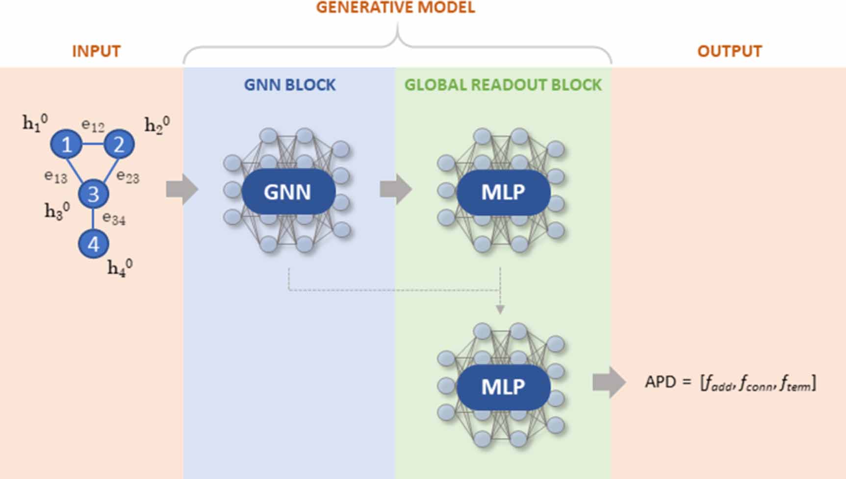
**Figure I5.** Example of structures randomly selected from the MOSES training set.
Download figure:
Standard image High-resolution image

Graph networks for molecular design

Article metrics

Submit

Share this article

Author e-mails

Author affiliations

ORCID iDs

Dates

Peer review information

Abstract

1. Introduction

1.1. Graph networks

1.2. Generative models

1.2.1. String-based generative models

1.2.2. Graph-based generative models

2. Methods

2.1. Model architecture

2.1.1. The GNN block

2.1.2. Global readout block

2.2. Model input and output

2.2.1. Model input

2.2.2. Model output

2.2.3. The graph decoding route

2.3. Training sets

2.4. Workflow

2.4.1. Preprocessing

2.4.2. Training

2.4.3. Generation

2.4.4. Benchmarking

2.5. Evaluation metrics

2.6. Hyperparameter optimization (HO)

2.7. Computational details

3. Results

3.1. Model evaluation

3.1.1. Canonical deconstruction path

3.1.2. Effect of dataset size

3.2. Benchmarking

3.2.1. Distribution-based benchmarks

3.2.2. Best model—cGGNN

3.3. Hyperparameter optimization (HO)

3.3.1. Transferability of hyperparameters

3.3.2. Optimizing the best model—the GGNN

3.4. Computational resource requirements

4. Discussion

4.1. Advantages of GraphINVENT models

4.2. Disadvantages of GraphINVENT models

4.3. Interesting observations

4.4. Comparing GNN performance

4.5. Avenues for future work

5. Conclusions

Acknowledgments

Data availability statement

Author's contributions

Competing interests

Code details

Appendix A.: Abbreviations

Appendix B.: Mathematical notation

B.1. Sets, tuples, and ordered lists

B.2. Tensors

B.2.1. GNN-specific tensors

B.3. Functions

B.4. Indices

Appendix C.: MPNN formulation

Appendix D.: Example representation

Appendix E.: Algorithms

Appendix F.: Hyperparameters

F.1. Hyperparameter optimization (HO) strategy

F.2. Default hyperparameters

Appendix G.: Evaluation metrics

G.1. Results for GDB-13 1K

G.2. Results for MOSES

G.2.1. Effect of dataset size

Appendix H.: GDB-13 1K experiments

H.1. Dropout in GDB-13 1K

H.2. Weight decay in GDB-13 1K

H.3. Canonical deconstruction in GDB-13 1K

Appendix I.: Examples of molecules

Footnotes