
Abstract
In this work, we use methods and concepts of applied algebraic topology to comprehensively explore the recent idea of topological phase transitions (TPTs) in complex systems. TPTs are characterized by the emergence of nontrivial homology groups as a function of a threshold parameter. Under certain conditions, one can identify TPTs via the zeros of the Euler characteristic or by singularities of the Euler entropy. Recent works provide strong evidence that TPTs can be interpreted as the intrinsic fingerprint of a complex network. This work illustrates this possibility by investigating various networks from a topological perspective. We first review the concept of TPTs in brain networks and discuss it in the context of high-order interactions in complex systems. We then investigate TPTs in protein–protein interaction networks using methods of topological data analysis for two variants of the duplication–divergence model. We compare our theoretical and computational results to experimental data freely available for gene co-expression networks of S. cerevisiae, also known as baker's yeast, as well as of the nematode C. elegans. Supporting our theoretical expectations, we can detect TPTs in both networks obtained according to different similarity measures. We then perform numerical simulations of TPTs in four classical network models: the Erdős–Rényi, the Watts–Strogatz, the random geometric, and the Barabasi–Albert models. Finally, we discuss the relevance of these insights for network science. Given the universality and wide use of those network models across disciplines, our work indicates that TPTs permeate a wide range of theoretical and empirical networks, offering promising avenues for further research.
Export citation and abstract BibTeX RIS

Original content from this work may be used under the terms of the Creative Commons Attribution 4.0 licence. Any further distribution of this work must maintain attribution to the author(s) and the title of the work, journal citation and DOI.
1. Introduction
Topology is the branch of mathematics concerned with finding properties of objects that are conserved under continuous deformations. The topological properties of a system are usually global properties that are independent of its coordinate system or a frame of reference [1]. There is a vast literature in theoretical physics relating phase transitions to rigorously mathematical topological changes in continuous and discrete systems. Research in continuous systems was made using tools of Morse theory [2–7], while applications in discrete systems relate to percolation theory [8–12]. Over the past years, the increasing availability of technology and new experimental methods has led to a massive data production that requires high processing power and the development of new methods and concepts to analyse them. In this context, topological data analysis (TDA) emerges as a promising methodological tool in complex systems [13, 14]. In this work, we bridge rigorous results from stochastic topology and statistical mechanics with recent TDA insights to showcase that topological phase transitions (TPTs) are ubiquous in complex systems.
Research on phase transitions in the context of stochastic topology started with the work of Erdős and Rényi [15], which investigates the problem of tracking the emergence of a giant component in a random graph for a critical probability threshold. Using methods from algebraic topology, one can generalize the basic concept of graphs to simplicial complexes, i.e., a set of points, edges, triangles, tetrahedrons and their n-dimensional analogues, which was later used by Kahle [16] and Linial and Peled [17], among others [18], to rigorously extend the giant component transition to a simplicial complex. In this new language, the generalization of the giant component transition constitutes a major change in the distribution of k-dimensional holes, i.e., the emergence of non-trivial homology groups in a simplicial complex, which are characterized by their k-Betti numbers, βk .
A central metric in this work is the Euler characteristic (EC), which is defined as the alternating sum of the quantities of k-dimensional simplices in a simplicial complex. In short, we can compute the EC of a complex network by associating it with a simplicial complex. We can identify the (k + 1)-cliques, i.e. the all-to-all connected subgraphs with k + 1 nodes in a network, with its k-dimensional simplices, thus obtaining the so-called clique complex. Therefore, if we denote Clk as the total number of k-cliques in a complex network (i.e., edges, triangles, tetrahedrons, etc), the EC, χ, is given by [19–21]

It has been ubiquitously observed that the logarithm density of the EC, log(|χ|), presents singular behaviour around the thermodynamic phase transition in theoretical models [2, 22], as well as around the zeros of the EC [10, 23–26]. This intuitively led to the introduction of TPTs in simplicial complexes as the loci of the zeros of the EC [27], where it was observed that the zeros of the EC also emerge in the vicinity of the generalization of the giant component transition [17]. In particular, it was observed that the zeros of the EC are also associated with the emergence of giant cycles in a simplicial complex [18, 28, 29]. Those transitions can be seen as one possible generalization of percolation transitions to higher-dimensional objects and were observed for the random clique complex of the Erdős–Rényi graph, as well as in functional brain networks [27]. Later, TPTs were also investigated across different domains, such as financial networks [30], collaboration networks [31], and astrophysics [32], to name a few. Recent developments on high-order interactions in network science [33–35] provide strong ground to further explore TPTs in complex systems.
In this work, we explore the topological transition across a variety of models, and discuss some applications in complex systems. We first review TPTs in the context of brain networks, since this was the first complex system where TPTs were observed, and discuss challenges of TPTs in brain networks in the context of high-order interactions in complex systems.
Second, as an exemplary case for the ubiquity of phase transitions in complex systems, this work studies the EC and its TPTs in two variants of protein–protein interaction networks (PPINs) models, as well as empirical data. PPINs are networks in which the nodes are proteins and the edges represent interactions between them. Topological properties of PPINs have been the subject of many relevant studies [36–38]. Here, we study TPTs in two analytical models of PPIN growth: the totally asymmetric and the heterodimerization duplication–divergence (DD) models [39, 40]. Moreover, to check whether the topological transitions identified are consistent with real PPIN data, we apply the same approach to data of yeast gene co-expression networks (GCNs) freely available online from the project Yeastnet v3 [41]. A GCN is a PPIN in which the edges are based on experimental measures of correlation between the activity of genes over different conditions [42]. We then study the TPTs in the heterodimerization model [40], a variant of the DD model, and compare our results with the phase transitions displayed in the C. elegans database [43].
Third, and lastly, we investigate the emergence of TPTs in four classical network models that are widely used for network analysis across research fields and scientific disciplines: the Erdős–Rényi graph, the Watts–Strogatz model, the random geometric graph, and the Barabasi–Albert model. Hereby, we seek to illustrate that TPTs permeate complex systems and might become a useful methodology to characterize the structure and intrinsic properties of complex networks.
This manuscript is written as follows: in section 2 we review and provide perspectives on TPTs in functional brain networks. Expanding our approach from the brain to a larger number of complex systems; in section 3 we introduce the PPINs, discuss the DD models and study phase transitions in PPIN through the totally asymmetric model; in section 4 we explore TPTs in yeast GCNs; and in section 5, we mobilize the heterodimerization model and apply it to data on the nematode C. elegans. Moving from PPIN to broader theoretical and simulated models, in section 6, we study the TPTs in four classical complex network models. Finally, section 7 offers our concluding remarks.
2. TPTs in functional brain networks
Functional brain networks are usually constructed by measuring correlations, or any similarity measure, between times series of activity of brain regions in resting state (or task based) fMRI [44–46]. Functional brain network organization can be described by the topological structure of the network, which includes nodes, edges, triangles, and even higher-dimensional objects. Given this structure, over the past years, methods of applied algebraic topology have been used to associate simplicial complexes to the study of the brain across multiple scales [47–52]. For instance, one can find multiple applications of algebraic topology in neuroscience, e.g., in psychedelics [53], neuronal dynamics [54], brain artery trees [55], epilepsy [56], and schizophrenia [57], to name a few. Yet, numerous significant concepts from algebraic topology and discrete geometry, especially stochastic topology [18], remain to be explored in neuroscience.
A natural question that emerges in this fertile line of research is whether high dimensional objects may also manifest phase transitions, both in structure and high-order dynamics. This possibility has been mostly shown at a theoretical and modelling level, and remains empirically underexplored. On the one hand, the work of Kahle [16], as well as Linial and Peled [17] generalized the percolation transition introduced by Erdős to simplicial complexes, which gave rise to recent developments in the field of stochastic topology [18], yet to be fully explored in complex systems. On the other hand, high-order extensions of dynamical systems have been proposed over the past years [33, 58]. In fact, one common feature of high-order dynamics [59] and structure [17] is the presence of first-order transitions induced by high-order interactions. This was already observed in multiple works on dynamics of systems with high-order interactions [60–69]. Translating this burgeoning work in stochastic topology to empirics, we recently observed TPTs by building simplicial complexes from resting-state fMRI brain networks. We found that functional brain networks undergo TPTs as a function of their intrinsic correlation level or edge density.
As discussed in the previous section, TPTs occur when the entropy of the network reaches a singularity, resulting in the formation of multidimensional topological holes in the brain network. In a functional brain network, each node corresponds to a different region in the brain, and a connectivity matrix is defined by a N × N matrix Cij of correlations between areas i and j in the brain, which is built from BOLD signals of rs-fMRI time series [70]. To analyse a brain network as a function of correlation level or density and study its associated simplicial complex, it is important to introduce the concept of filtration: for a given ɛ ∈ [0, 1], this process requires the removal of all edges with correlation of at least 1 − ɛ. For ɛ = 0, for example, we would have an empty network, with all the nodes disconnected. As ɛ increases, we include the links with a correlation greater than 1 − ɛ. We illustrate the idea of a filtration in figure 1. In this figure, each frame has edge density equal to 0.0%, 0.5%, 1%, and 2.5%, respectively. In [27], we use this idea of filtration to establish an analogy between the functional brain network and Hamiltonian physics by understanding correlation levels in the brain network as energy levels in a Hamiltonian physical system or as height function in Morse theory and computational topology [71]. It is important to note that there is no unique way to define filtration in a complex system, and this choice is often problem-dependent. In some applications, more than one filtration scheme was implemented in empirical data, see, e.g., [27, 72]. In stochastic topology, using probability as a filtration parameter for theoretical models is common [16]. However, different similarity measures can be chosen as a parameter for filtration in empirical data, such as distance, network density, correlation or mutual information, etc.
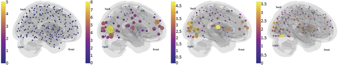
Figure 1. Illustration of filtration in a functional brain network. We first start with an empty brain network and build a nested chain of networks. In each step, we add the strongest k-simplices, which in this work are k-cliques, for a fixed density. Each frame has edge density equal to 0.0%, 0.5%, 1%, and 2.5%, respectively. Data visualizations of high-order brain networks illustrated in this work were created using methods developed in [27, 73] and are freely available in [74].
Download figure:
Standard image High-resolution imageThere are multiple ways to define a simplicial complex from brain network data [33, 58, 75]. The one illustrated in figure 1 is perhaps the simplest one, which is made by enumerating the cliques of a functional brain network in each step of the filtration. 0-simplexes are nodes, one-simplexes are edges and so on. In figure 2, we illustrated three- and four-simplexes using brain network data from the human connectome project (HCP) project [76, 77], as done in [27, 73].

Figure 2. Simplicial complexes and high-order interactions in functional brain networks: we illustrate (a) three-cliques and (b) four-cliques. Each figure has edge density equal to 0.6% and 1.3%, respectively. Data visualization tools were developed in [27, 73] and are freely available in [74].
Download figure:
Standard image High-resolution imageWe now move to the study of TPTs in functional brain networks, defined as the loci of the zeros of the EC or the singularity of the Euler entropy. In figure 3(a) (from [27]), we illustrate the TPTs for individuals in the HCP. We note that the first transition corresponds to the classic Erdős–Rényi percolation transition, whereas the second transition corresponds to the emergence of high-order loops, analogous to what was proposed rigorously by Linial and Peled for a random simplicial complex [17].

Figure 3. (a) TPTs in rs-fMRI brain networks of 420 individuals in the HCP project. Reprinted figure with permission from [27], Copyright (2019) by the American Physical Society. (b) Distribution of node curvature at the vicinity of the second phase transition.
Download figure:
Standard image High-resolution imageThese findings on TPTs trigger a question about the relationship between the global and local properties of brain networks at the vicinity of a phase transition. In particular, k-cliques are a key element in the analysis of brain network organization and function. For instance, we can analyse, for each brain region, the number of k-cliques that this region participates in as a function of the correlation between brain regions [51]. For example, in figure 2, the size of the nodes are proportional to their participation rank in k-cliques.
Our work shows that the local network structure and the local node participation rank are related to the TPTs in the human brain network. In fact, one can associate local curvature to a brain network. There are multiple ways of defining discrete curvature in a network [78]. However, in this work, we use the curvature of complex networks as a local version of the EC in the context of the Gauss–Bonnet theorem proposed by Knill [79]. In figure 3(b) we illustrate the distribution of curvature at the nodes of the functional brain network at the vicinity of a phase transition. We find that the Gauss–Bonnet theorem holds for all values of ɛ between the first and second transition. In the online supplementary material (https://stacks.iop.org/JPCOMPLEX/3/025003/mmedia), you can find a video with the evolution of the curvature as a function of the density of the network.
Another relevant feature of the Euler entropy are its local maxima, which can be seen as an estimation of the maximum number of loops in a real network for a given dimension. For instance, the first local maxima estimates the maximum number of clusters, the second the maximum number of cycles, and so on. In neuroscience, more specifically in cerebral blood flow studies in PET scans, the number of isolated regions of activation above a given threshold is estimated by the local maximum of the EC, see [80].
An interesting aspect of TPTs that relates to theoretical physics is that critical points of a phase transition are universal and can therefore be used as markers for a material or substance. In neuroscience, these findings on TPTs were used to distinguish between functional brain networks of healthy control individuals and individuals with Glioma [27]. Later, TPTs were also used as topological markers for identifying differences between ADDH and typically developing individuals [81], as well as in EEG measurement to identify individuals responding to different contours and shapes in images during Gestalt cognitive tests [82]. Together, those results indicate that TPTs are a potential biomarker in functional brain networks and, as we will discuss in the next section, in complex systems more generally.
3. From protein interaction networks to the DD model
Building upon this discussion of recent findings on TPTs in functional brain networks, we now move on to the analysis of TPTs in other complex systems, starting with PPINs. Proteins are macromolecules that participate in a vast range of cell functions, such as DNA replication, responses to stimuli or even the transport of molecules. The interaction between proteins represents a central role in almost every cellular process [83]. For instance, understanding how proteins interact within a network can be crucial to advance the identification of cells' physiology between normal or disease states [84].
Interactions between proteins in a cell can be mathematically represented as a network (or graph), a mathematical structure composed by nodes (or vertices) and edges (or links). In this framework, proteins are the nodes and each pair of interacting nodes are connected by an edge. This representation is often referred to as a PPIN [36]. In figure 4, we illustrate a GCN for yeast using Cytoscape [85].
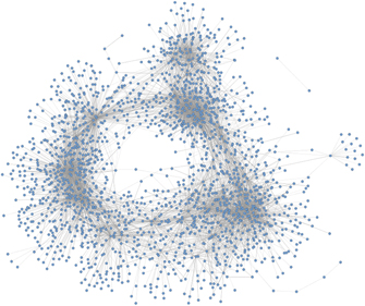
Figure 4. Network representation of GCN for yeast using Cytoscape [85]. The presented yeast network has 1893 nodes, 7955 links and it was obtained from Yeastnet v3 [41].
Download figure:
Standard image High-resolution imageIn [36] it was first observed that PPIN behave similarly to scale-free networks, i.e., that there are a few nodes participating in the majority of cellular functions. Those nodes are connected to many other nodes and have a high degree, the so-called hubs. In fact, this scale-free property can be observed in a range of other complex systems, like the world wide web or social networks [86]. The emergence of such systems is characterized by continuous growth and a preferential attachment principle: new nodes are always added to the system and have a higher propensity to attach to nodes with a higher degree, resulting in a power-law degree distribution. In such distribution, the fraction p(k) of nodes with degree k in the network is inversely proportional to some power of k. In PPIN, this scale-free topology is reported to be a consequence of gene duplication [87].
Gene duplication is the process that generates new genetic material during molecular evolution. We can assume that duplicated genes produce indistinguishable proteins which, in the network formalism, implies that new proteins will have the same link structure as the original protein. Every time a gene duplicates, the proteins that are linked with the product of this gene have one extra link on the network. Thus, proteins with more links are more likely to have a neighbour to be duplicated.
The discovery of a scale-free property in PPIN gave rise to many models for generating PPIN based on the gene duplication principle [39, 40, 88–90]. Most of these models rely on divergence, a process in which genes generated by the same ancestral through duplication accumulate independent changes on their genetic profile over time. The so-called DD models were first introduced in [88]. The models are based on the observation that PPIN grow after several gene duplication that can occasionally diverge in their functions over time. There are some variants of this model, which include for instance heterodimerization, arbitrary divergence [40] and random mutations [89].
The totally asymmetric model is defined as a DD model in which the divergence process is assumed to happen only on the replica of the duplicated node. This model, proposed in [39], is based on the hypothesis that, after duplication, there is a slight chance that the replicate node starts to develop different functions from the original one. In the model, this change is indicated by the deletion of some edges from the replica and is supposed to happen a single time during the growth of the network. The growth of the network according to this model is illustrate in figure 5 and it is defined as follows: given a number N of proteins and a probability p (0 ⩽ p ⩽ 1), the model generates a graph with N nodes starting from a single one, following the presented algorithm:
- Duplication: one node, as well as its edges, is randomly selected to duplicate.
- Divergence: each duplicated edge that emerges from the replica is activated with a retention probability p. The non-activated edges are removed from the network.
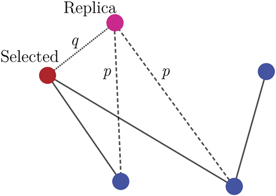
Figure 5. Illustration of a duplication step in PPIN model. For each duplication step, a node is selected to be duplicated (red) with its edges. Each new duplicated edge (dashed lines) that goes from the replica (pink) can be activated with independent probability p and the non-activated edges are removed. Additionally, for the heterodimerization model discussed in section 5, an edge going from the replica to the original node (dotted line) is created with probability q.
Download figure:
Standard image High-resolution imageThe duplication step aims to capture genetic replication in a cell, while the divergence step simulates the possibility of a mutation after duplication, which can generate new proteins performing different functions than the original. Some authors [39] consider that any duplication that leads to an isolated node should not be considered. However, since isolated nodes are also considered when computing the EC, we kept them to guarantee consistency between theory and experiment. In fact, this approach provides a different perspective on gene co-expression data modelling. As we will verify further, experimental data shows isolated nodes for lower levels of co-expression (≪1). As we illustrate below, keeping the isolated duplicated nodes will make the modelling more appropriate to match TPTs in the model with the experiments.
For the computation of the EC (or equivalently the Euler entropy), observe that since new duplicates are not linked to their ancestors, the DD algorithm will only produce bipartite networks, which implies that the networks will not have cliques with size 3 or greater [40]. The EC, therefore, will be reduced to the formula χ = N − E, where N represents the total number of nodes, and E the total number of edges of the network. This simplicity enables us to analytically obtain the expected mean value of the EC in terms of the probability p for a graph with N nodes, by

The expected value for the number of edges as function of p for a totally asymmetric model with N nodes is given by (see

Since the Euler entropy is given by Sχ = log|⟨χ⟩|, we have a singularity on Sχ at the values of p where ⟨χ⟩ = 0, i.e., where

A network that has more edges than nodes certainly has cycles [91]. So, the first topological transition point marks the exact retention probability at which it is highly probable that the network has cycles, i.e., in the vicinity of the emergence of a giant component in the network [15].
In figure 6, we observe the behaviour of Sχ
as a function of the probability p of the totally asymmetric model, for a network with 1000 nodes. One can observe that there is a single singularity when p reaches the critical value of  (dashed black line), in the vicinity of the critical probability of the giant component transition.
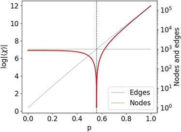
Figure 6. Euler entropy Sχ = log|⟨χ⟩| as function of the retention probability p for the DD model with 1000 nodes. Sχ was determined by (2). The singularities Sχ → −∞, or the zeros of χ locate the TPTs on the DD model. We put the number of nodes and edges in a logarithmic scale to make visible the change of domain between the number of nodes and the number of edges that occurs at the phase transition's critical probability.
Download figure:
Standard image High-resolution imageTo characterize this phase transition and understand its implications, we analyse the model through another topological parameter, known as Betti numbers. In general, Betti numbers, indicated by βn , are defined as follows: β0 is the total number of connected components. β1 is the number of cycles on the graph. For n > 1 the structure becomes more complex, but roughly speaking, βn indicates the number of n-dimensional 'holes' in the network [19, 71].
Figure 7 presents the behaviour of the Betti numbers β0 and β1 as functions of p compared with the EC. Here, we were not able to achieve an analytic expression for the Betti numbers, they were obtained numerically by generating and averaging 1000 simulations for each value of p (from 0.0 to 1.0 at steps of 10−2), 1000 nodes each.
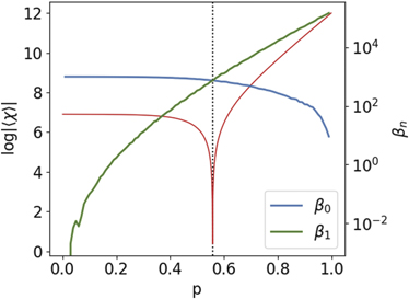
Figure 7. Betti numbers β0 and β1 for the DD model as function of the retention probability p (N = 1000). At the first phase the network is fragmented, with many components. As p increases, β1 (i.e., the number of cycles) surpasses β0 when p crosses the transition point, indicating a major change in the topology of the DD graph.
Download figure:
Standard image High-resolution imageNote that the topological transition occurs in the vicinity of the value of pc where the Betti curves β0 and β1 overlap and, consequently, χ = 0, thus confirming the results introduced theoretically in the context of stochastic topology [16–18]. For p < pc the network is divided into many components because there is a high chance that duplicated nodes do not connect with any neighbour of the original nodes. As p increases, the number of components decreases and we have an abundance of cycles in the network. Near pc, the expected number of cycles is as big as the expected number of components, so there is a high chance that the graph has a cluster with  nodes.
Another interpretation for the phase transition obtained from the totally asymmetric model comes from percolation theory. It is a known fact that the first change of sign of the EC in complex networks is related to the appearance of a giant component, i.e., of a connected component in the graph that involves a significant part of the nodes in the system. In the totally asymmetric model, we observe a similar relation, as the TPT obtained is the percolation transition of the system, i.e., the value of the probabilistic parameter that maintains most of the proteins interacting as a whole.
4. Gene co-expression networks
In a biological context, interactions among proteins can be physical interactions, indicated by the physical contact between them as a result of biochemical events guided by electrostatic forces [92], but also functional interactions. In fact, a group of proteins can perform a common biological function without actually being in direct contact, regulating a biological process or making common use of another molecule [83].
To identify functional interactions, a common method consists in analyzing gene co-expression patterns. This method is based on the assumption that genes with correlated activity produce interacting proteins [93]. Therefore, by mapping the correlation between the activity of genes, we can build the so-called GCN [83].
A GCN is a PPIN in which the edges are based on experimental measures of correlation between the activity of genes over different conditions. Each node of the network corresponds to a gene. An edge connects a pair of genes if they present similar expression patterns over all the experimental conditions [42]. GCNs are often used to identify groups of genes that, over various experimental conditions, display correlated expression profiles. Based on the 'guilt-by-association' principle [94], it is possible to hypothesize that those genes share common functionality. Therefore, the understanding and comparison of topological features across co-expression networks may provide useful information about the strengths (and weaknesses) of the theoretical models used to infer different co-expression networks [95].
We now contrast the theory and numerical simulations presented in the previous section with GCNs obtained experimentally from data for yeast networks available in [41]. Our aim is to test whether we observe similar topological transitions on real data of GCN, and what insights such transitions provide us about the structural properties of the network.
Here, we analysed 48 empirical GCNs from S. cerevisiae, also known as baker's yeast, available online from the project YeastNet v3 [41]. The whole data set covers around 97% of the yeast coding genome (5730 genes). The networks in this dataset have between 800 and 3000 nodes and between 7000 and 64 000 links. They were collected through diverse experimental approaches. Each of the datasets analysed consists of one weighted adjacency matrix for the yeast network. Each node on this network corresponds to a gene. Two genes are connected by an edge if there is a significant co-expression relationship between them. We associate to each edge a weight that corresponds to the absolute value of the correlation between the expression levels of the nodes in the network.
After creating a GCN from the co-expression matrices, we proceed with a numerical process called filtration. For a given ɛ ∈ [0, 1], this process requires the removal of all the edges with correlation, i.e., edges' weights, at most 1 − ɛ. For ɛ = 0, for example, we would have an empty network, with all the nodes disconnected. As ɛ increases, we include the links with a correlation greater than 1 − ɛ. We perform this procedure until ɛ reaches 1 and the network becomes fully connected. In this paper, we used the filtration process to track how the topology of the GCN changes as a function of the correlation between the genes.
In contrast to the results of the previous case, where the EC was written analytically as a function of the probabilistic parameter p for the totally asymmetric model, the EC can be obtained numerically as a function of a parameter ɛ, such that Clk = Clk (ɛ) and consequently χ = χ(ɛ) in equation (1).
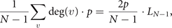
As the computation of topological invariants is an NP-complete problem [96], here, we only illustrate datasets where the computation was feasible, namely, to 20 yeast networks. Figure 8 shows the Euler entropy as a function of ɛ for the 20 selected networks on Yeastnet's database. The time scale for the numerical computation of the numbers of k-cliques increases exponentially with the size of the network. This occurs because, as ɛ increases, the network becomes denser, and the computation of the cliques become extensive. For this reason, in some of the datasets, we could not compute the EC to a threshold where one could detect a TPT. Nonetheless, the Euler entropy averaged over the data sets (blue line) clearly shows the presence of a singularity.

Figure 8. Euler entropy Sχ as a function of the correlation threshold ɛ for 20 GCNs from Yeastnet database. Each gray line corresponds to a unique co-expression network, while the blue line is the average of the gray ones. Most of the TPTs were detected on those networks for ɛ in the average critical value ɛ ≈ 0.876, except for the yeast network with DNA damage, where the transition happens for ɛ ≈ 0.573 (red curve). This particular experiment was designed to measure the response to DNA damage in the network [97], and the shift in the critical threshold of the topological transition is apparently sensitive to that response.
Download figure:
Standard image High-resolution imageObserve that most of the singularities happen near ɛ ≈ 0.876 except for one of the networks, in red, where the singularity happened at ɛ ≈ 0.573. This network comes from an experiment whose goal was to evaluate response to DNA damage due to methylmethane sulfonate and ionizing radiation [97]. In fact, it is known that eukaryotic cells respond to DNA damage by rearranging its cycle and modulating gene expression to ensure efficient DNA repair [97]. Therefore, our analysis suggests that the Euler entropy could be sensible to this reorganization process in the damaged yeast network. The purpose of this empirical example is to illustrate the methodology, and therefore further investigation of the relationship between GCN with DNA damage and percolation transitions will be an important step to establish whether the zeros of the EC can be used as a topological bio-marker of such systems, with the potential to detect DNA damage.
In order to provide a deeper characterization of the TPT of GCNs, we also calculated the Betti curves β0 and β1 for the same yeast networks. From a theoretical perspective, a TPT should occur at the vicinity of the zeros of EC and when β0 ≈ β1. In figure 9, we illustrate the averaged Betti curves for the above-mentioned dataset.
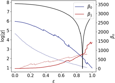
Figure 9. Average Betti curves (β0 and β1 as a function of the correlation threshold ɛ). Observe that, as with the totally asymmetric model analysed previously, the domain of β0 and β1 shifts at the vicinity of the singularity of the Euler entropy (black line), i.e., at the zeros of the EC. Dotted lines correspond to the Betti numbers of the yeast network with DNA damage.
Download figure:
Standard image High-resolution imageWe can observe agreement between the threshold transition of Sχ and the threshold where β1 ≈ β0, in analogy with the topological transitions reported for theoretical models of random simplicial complexes [17, 98] and for functional brain networks [27].
For values of the correlation threshold below the transition, the network is fragmented in many components, since β0 is greater than β1. As ɛ gets closer to the transition, more edges are added to the network, lowering the number of connected components, and changing the network structure to a denser one and with more cycles, i.e., higher β1. Once the number of connected components approaches 1, i.e., β0 → 1, almost every new edge has a high probability to create more loops, and the topological transition happens precisely when the number of loops (β1) is greater than the number of connected components (β0).
These observations about the behaviour of Betti numbers are compatible with the results observed in [99], and provide some possible interpretation for this shift at the critical point of the TPT. In [99] a linear correlation of R = −0.55 was observed between the chance of survival of cancer patients and the number of cycles in the network, also known as the complexity of the cancer PPIN. In fact, the complexity was measured using persistence homology, specifically the magnitude of the Betti number β1, which counts the number of one-dimensional cycles in the network. The higher β1, the higher is the complexity, which implies lower chances of survival [99]. This study provides evidence that, for cancerous cells, the complexity of the PPIN is associated with the health state of the cell.
Now, returning to our analysis of yeast GCNs, we observed that, for one of the networks, the transition indicated by the EC happened at a distinct threshold  . The analysis of the Betti numbers indicates that this transition is characterized by a shift of dominance between β0 and β1, as theoretically described for random simplicial complexes [17]. Thus, during the filtration process, the network corresponding to yeast with DNA damage reaches the TPT earlier than the other data (where the transitions happened near ɛ ≈ 0.876), indicating a rapid appearance of cycles in the network, i.e., the increase of network complexity.
It is important to mention that there are more suitable methods to detect DNA damage, for example, measuring the expression of genes in the DNA repair pathway. But, even though further experimental studies are desired to evaluate the statistical significance of the shift in TPTs for yeast PPIN under DNA damage, our results suggest that phase transitions are indeed intrinsic properties of the system and seem to be sensitive to DNA damage. Together with recent results on brain networks [27, 81] and on cancerous cells discussed in [99], our results reinforce the hypothesis that TPTs have the potential to be used as intrinsic biomarkers for protein interaction networks more generally.
5. Heterodimerization model and C. elegans
We now move towards a model where protein interactions display more complex dynamics and could potentially capture different empirical data for PPIN. In fact, this model is a variation of the totally asymmetric model discussed in the previous sections. Applied to networks, the model is described as follows: given a number of nodes N and two probabilistic parameters p and q, the model generates a graph from two nodes and a single edge following the steps below, illustrated in figure 5:
- DD steps are equal to those in the totally asymmetric model (see section 3).
- Heterodimerization: the replicated and the original nodes can connect with probability q.
The heterodimerization step mimics the probability that the original node is a dimer, i.e., two molecules joined by bonds that can be either strong or weak. This step is important for clustering and is observed in real PPINs [100]. It is also known that this model produces cliques with similar size and quantity to those observed in some real PPINs [40], contrasting with the totally asymmetric model where we could only observe cliques with small sizes.
As previously defined, the phase transitions are the singularities of the Euler entropy. Given the complexity of the distribution of cliques in these models [40], we were only able to generate these networks numerically, and we further compared them with experimental data. In figure 10(a), we observe the average of the Euler entropy Sχ as a function of the retention probability p for a representative network with 1000 nodes and different values of q. We see that the heterodimerization parameter q induces the emergence of further TPTs. These additional TPTs emerge because the heterodimerization step makes possible the appearance of cliques of higher order. The higher the value of q, the more probable it becomes for cliques of larger sizes to appear and, therefore, the higher is the likelihood of further TPTs. In this context, it is important to note that [101] reports the abundance of large cliques in real PPIN data, which makes the heterodimerization model more compatible with empirical data.
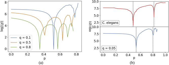
Figure 10. Euler entropy of the DD model with heterodimerization. (a) Average of the Euler entropy as function of the retention probability p for different values of q. Note that, in contrast to the previous model, there are more transitions as we increase the value of q. This is because the heterodimerization step makes it possible for cliques of different sizes to appear, as observed in real PPINs [40]. (b) Euler entropy of PPIN from C. elegans (top) in contrast with an illustrative simulation for the heterodimerization model with q = 0.05 (bottom). Both have two singularities.
Download figure:
Standard image High-resolution imageGiven the bigger size, higher number and complex distribution of the high-dimensional cliques in this model, we were not able to achieve an analytic expression for the Euler entropy. Also, since the network becomes denser due to the heterodimerization step, we did not compute the Betti numbers as we did for the totally asymmetric model. Nevertheless, to reinforce the significance of our analysis, we compare our numerical simulations to experimental data for PPIN which, in fact, presents a similar phase transitions profile.
In figure 10(b) (top) we illustrate the Euler entropy of a PPIN for the C. elegans. The data for this nematode was obtained from the Wormnet v.3 database [43]. For this network, which consists of 2219 genes and 53 683 links, each link was inferred by analysis of bacterial and archaeal orthologs, i.e., homologous gene sequences of bacteria and archaea related to C. elegans by linear descent.
Differently from the data of yeast GCN presented previously, the Euler entropy of this network presents two singularities at the vicinity of ɛ1 = 0.48 and ɛ2 = 0.82. This behaviour could not be observed if we would consider the growth of a PPIN through DD only. However, with the heterodimerization model, we were able to achieve a similar profile of the Euler entropy by simply setting the representative parameters, as can be seen at the bottom of figure 10(b), which shows the expected Euler entropy as a function of the retention probability p, averaged over 1000 simulations for each value of p (ranging from 0 to 1 with steps of 10−2). For this simulation, we set the number of nodes at 2219 so that we can compare it with the C. elegans empirical data. We also set the value of the heterodimerization probability q to 0.05. Even though this value was only set for comparison purposes, not intending to perform an optimal fit to the empirical data, it is within the same order of magnitude of the value of q = 0.03 used in [40], where the authors managed to achieve a good approximation for the clique distribution across the PPIN considered.
Even though the DD model was enough to understand the topological properties of the yeast networks in the previous sections, it is important to mention that dimerization also happens during the growth of such networks. However, this process is not frequent enough to produce significant quantities of big cliques, which would result in new TPTs. This analysis suggests that during the growth of the C. elegans network, dimerization happened more frequently, in a way that the DD model could not reproduce such topological properties. Therefore, the TPTs displayed by the heterodimerization model are more appropriate for this specific empirical network. We notice that, in order to match our theory and numerical simulations to the experimental data, we considered that the nodes that got isolated after duplication were kept in the network.
It is important to emphasize that other models suggest different processes for PPIN growth, implying that our analysis did not exhaust the possibilities of models considered for PPIN. In [40] for example, the authors present an arbitrary divergence model in which they could replicate with high confidence the clique distribution observed for PPIN data. Other models simulate different aspects of the growth of a PPIN [40, 89, 90] and the analysis of such models through the lenses of TPTs and the EC would give us precious information about PPIN.
Our theoretical and empirical analysis of complex biological networks reinforces the strong evidence that the zeros of the EC can be interpreted as an intrinsic fingerprint of a given network. This suggests that TPTs have the potential to be a critical tool to characterize complex systems more generally.
6. TTP in classical network models
In the remainder of this paper, we illustrate how commonly used complex network models also display TPTs and can be studied using the zeros of equation (1), the EC χ. In the previous sections, we showed that TPTs were associated with the log|⟨χ⟩| of the PPIN using the DD and the heterodimerization models [88], which were subsequently compared against empirical data. Here we investigate the TPT in the Erdős–Rényi model, the Watts–Strogatz model, the random geometric model, and the Barabasi–Albert model. Together, these models capture a wide range of phenomena in network science across numerous fields, such as small-world property, percolation transitions, preferential attachment, to name a few.
From a computational perspective, topological transitions require the use of an ensemble with many replicas for each set of parameters in each model. In this section, we fixed an amount of 100 replicas per system studied. Note that the number of simplices increases exponentially with the addition of edges to the network. Therefore, without limiting the size of the clique in our computation, we needed to find over 1011 simplices per model analysed (see figure 11), which is obviously a non-trivial computational problem.

Figure 11. TPT for classic network models: (a) the Erdős–Rényi model for 0 ⩽ p ⩽ 0.5. (b) The Watts–Strogatz small-world model, for two values of first neighbours connections k, namely k = 100 (continuous lines), and k = 50 (dashed lines). (c) The random geometric model in D = 3 as well as (d) the Barabasi–Albert model. The averages were obtained from 100 realizations for each parameter, green lines are the number of simplices found, red lines the Euler entropy, and gray lines represent individual realizations for each network.
Download figure:
Standard image High-resolution image
The observation of topological transitions in such models is, therefore, a critical step towards the use of such methodology in complex systems more generally. Moreover, the topological transitions described here are of great interest for a better understanding of high-order interactions in complex systems [34, 102–107].
TPT in the Erdős–Rényi model: in the Erdős–Rényi network, any two nodes are connected by a linking edge with independent probability p. The simplicial complex of the Erdős–Rényi graph, in which all cliques are faces, was investigated rigorously in [16, 27] for fixed N nodes as a function of the probability parameter p ∈ [0, 1]. If p = 0, there are no nodes connected (empty graph), whereas for p = 1, we have a complete graph. In figure 11(a), we illustrate the TPT of the Erdős–Rényi networks for N = 500 nodes and 0 ⩽ p ⩽ 0.5. We can see several singularities in the Euler entropy associated with the many zeros of the mean EC. The averages were obtained from 100 realizations for each parameter, green lines are the number of simplices found, red lines the Euler entropy, and grey lines represent individual realizations for each network.
TPT in the Watts–Strogatz model: to bridge the empirical analysis of protein structures and the discussion of theoretical network models, we now explore the classical Watts–Strogatz network, a small-world model that can also be used to study PPIN [108–110].
The small-world model is constructed from a ring with n nodes, and each node is connected with its k first neighbours if k is even, or k − 1 neighbours if k is odd. After that, each edge is randomly rewired with probability p ∈ [0.0, 1.0]. Once these networks are built numerically, we can study the topological transitions displayed by this network as a function of the rewiring probability. In fact, we show in figure 11(b) that a small-world network of n = 500 also displays the TPT observed in the previous section.
We can proceed with a more detailed inspection of the Watts–Strogatz model by changing the number k of first neighbours. For k = 50, figure 11(b) shows only one transition. Increasing the number of first neighbours to k = 100, we can see at least four transitions. Observe that real-world data sometimes has few nodes to be analysed, and the use of 500 nodes and the ability to differentiate among different topologies (as observed in the previous section) is a clear strength of the present methodology.
TPT in the random geometric model. Once studied through a small-world model, we can go further and investigate the topological transitions of the random geometric graph model in three dimensions [111]. This model is generated by using the number of nodes n and a distance r as inputs. First, one chooses n nodes uniformly at random in the unit cube, which are subsequently connected by an edge if the distance between them is lower than or equal to r. We can then study the topological transitions in this network as a function of the distance r.
We show the Euler entropy and its TPTs for the random geometric model in figure 11(c) for n = 500 nodes averaged from an ensemble of 100 replicas for each set of parameters. The zeros of the EC also correspond to changes in the signs of χ, which can be understood as changes in the sign of the mean curvature of the nodes [27] as described by the Gauss–Bonnet theorem for networks [20]. This interpretation can be important when we want to investigate topological changes in network models whose filtration parameter is not necessarily continuous, as we will see below.
TPT in the Barabasi–Albert model. Lastly, we illustrate the topological changes in the Barabasi–Albert network model [112]. This model is known for introducing random scale-free networks using a preferential attachment mechanism. The network starts with few nodes and no edges and a number of edges attached to the new node with probability proportional to the node's degree. In contrast to the three previous network models studied in this section, the Barabasi–Albert model has two integer parameters, namely, the maximum number of nodes n and the number of edges m which are attached to a new node during growth of the network. The attachment probability is proportional to the number of edges of the existing nodes.
We can analyse the topological transitions in the Barabasi–Albert network for a fixed n = 500 as a function of m. However, given the discrete nature of the control parameter m of this network model, we were only able to infer the TPTs via changes in the signal of the EC, which tracks the changes in the curvature of the nodes via the Gauss–Bonnet theorem for networks [20]. Figure 11(d) shows three zeros of the EC as a function of the number of edges attached using an ensemble of 100 replicas. Similarly to the random geometric graph, the transitions are revealed by a sign change of χ. Our inferred results for the first transition, m = 2, is in agreement with the percolation transition for the Barabasi–Albert model [113]. However, little is known regarding topological changes in the Barabasi–Albert model for higher values of m. For this particular model, one interesting analogy could be made regarding the relationship between Lyapunov exponents, curvature and phase transitions known in statistical mechanics [114, 115].
In fact, Lyapunov stability theory was adapted to the context of networks [116], and particularly to the Barabasi–Albert model [117], where the authors studied which values of m anomalous events occur in this network. We noticed that some of the critical intervals for m in [117] are analogous to the changes in the curvature as a function of m observed in our work. Therefore, the connection between reference [117] and TPTs deserves further investigation.
Ultimately, the aim of this section was to illustrate that topological transitions, evidenced by the zeros of the EC, are present in four classical network models that are widely used in network analysis across a variety of fields. This reinforces the ubiquity of such topological transitions in complex systems more generally.
7. Conclusions and perspectives
In this work, we investigated TPTs in a wide range of theoretical and empirical networks. TPTs are characterized by the zeros of the EC at a critical probability or threshold and represent a generalization of the giant component percolation transition introduced by Erdős [15–17] and recently expanded to data-driven complex networks [27]. The zeros of the EC also indicate signal changes in the mean curvature [20] and the emergence of giant k-cycles in a simplicial complex [28].
We first drew our attention to functional brain networks, where TPTs were empirically evidenced first. We then focussed our analysis on PPINs, particularly on networks generated by the totally asymmetric DD model. We verified that such transitions correspond to the emergence of a giant component in the network, as observed in yeast and GCNs datasets [41]. Then, we explored TPTs in the C. elegans PPIN. In contrast to the yeast networks, the same approach gave rise to two TPTs, indicating that the totally asymmetric model is insufficient to capture the topological aspects of the C. elegans PPIN data properly.
Our results give strong support to the hypothesis that percolation transitions are topological bio-markers of a network [27, 81]. In fact, by analyzing a network for yeast under DNA damage [97], we found that the transition point shifted to a much lower value compared to the interval in which the TPTs of the other yeast network datasets took place. Similar insights were reached when comparing functional brain networks of healthy individuals and individuals with Glioma [27], as well as with ADDH [81]. Although these results deserve further investigation, we provide evidence that the zeros of the EC can be seen as suitable topological invariants to distinguish macroscopic properties of yeast networks.
More generally, in order to further explore TPTs in complex systems, we extended our analysis to four classical network models, namely: the Erdős–Rényi model [15], the Watts–Strogatz model [108], the random geometric model [111], and the Barabasi–Albert model [112]. We showed that topological transitions permeate these models which are widely used across disciplines, and some of those transitions were not observed before by the analysis of classical networks using standard methodologies.
As discussed above, the geometric meaning of TPTs is related to high-order versions of percolation theory, especially within stochastic topology [16, 18]. From a theoretical physics perspective, the EC is also related to phase transitions in classic Hamiltonian systems studied in statistical mechanics [2, 4]. From a complex system perspective, given the recent introduction of TPTs [27], the meaning of those transitions is not fully known and depends on the specificity of the complex system itself. It can range from identifying crashes in financial networks [118], to characterizing image quality perception in EEG [82]. The connection between TPTs and other topics on high-order interactions in complex systems is also relevant. For instance, there are results connecting synchronization dynamics and percolation for regular networks [119]. Therefore, a proper connection between high-order percolation transition and high-order synchronization [59] may be also of interest.
We believe that the overview of TPTs reported in this work contributes to a better understanding of the ubiquity of topological transitions in real-world data and complex systems. Furthermore, we highlight the possibility of using algebraic topological methods, especially stochastic topology, to characterize those systems using high-order topological structures. Among the numerous directions for future works, we believe it would be particularly valuable to connect the results reported here with criticality, structure and dynamics in high-order networks and complex systems.
Acknowledgments
This work is funded by CAPES, CNPq, and FACEPE (Brazilian Scientific Funding Agencies). F A N Santos would like to express his gratitude for the useful discussions with Linda Douw, Mauricio D Coutinho-Filho, Ernesto P Raposo, Mauro Coppeli, James Charles Phillips, Stefan Boettcher, Bertrand Berche, Katharina Natter and Fernando Moraes during the development of this work. E C de Amorim Filho would like to thank V A Caldas and T Shimizu for the learn-full visiting period at AMOLF. We would like to acknowledge FACEPE Pronex APQ-0602-105/14 and FACEPE-Fulbright ARC-0103-1.01/17.
Data availability statement
No new data were created or analysed in this study.
Appendix
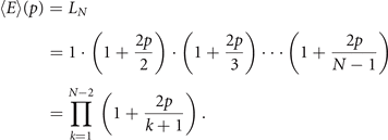
Proof of equation 3. Randomly selecting a node v on a network with N − 1 vertices, the expected increase in the number of edges after the divergence steps is

where deg(v) is indicating the number of nodes linked to v by an edge. So, if we want the expected increase after the DD steps, we just need to average over all nodes, giving us
where LN−1 is the number of edges before DD steps. Adding that to the edges we had before duplicating, we have that
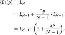
Now, remember that the algorithm starts with a graph with two nodes and a single edge, meaning that L2 = 1. So, using recursion, we can conclude that
□