
Abstract
This article presents a new version of transient behaviour occurring around the remnants of normally hyperbolic invariant manifolds (NHIMs) when they are already in the process of decay. If in such a situation a chaotic region of the NHIM is in the process of decay, then typical trajectories starting in this chaotic region remain in this region for a finite time only and will leave the neighbourhood of the NHIM in the long run in tangential direction. Therefore this chaotic region has a transient existence only as remainder of the NHIM. Numerical examples of this phenomenon are presented for a three degrees of freedom (3-dof) model for the motion of a test particle in the gravitational field of a rotating barred galaxy.
Export citation and abstract BibTeX RIS

Original content from this work may be used under the terms of the Creative Commons Attribution 4.0 licence. Any further distribution of this work must maintain attribution to the author(s) and the title of the work, journal citation and DOI.
1. Introduction
It is a common phenomenon in dynamical systems that generic trajectories perform some type of (possibly more complicated) behaviour for a finite time before they settle down to the distinct (frequently simpler) asymptotic long time behaviour. This effect is known under the name 'transients'. If the finite time behaviour is chaotic then we speak of transient chaos. For a detailed explanation of transient chaos in general see [1].
In Hamiltonian systems with their time reversal invariance we see the transition to the simple asymptotic behaviour in the future as well as in the past. The prototypical Hamiltonian case of transient chaos is chaotic scattering. In a scattering system the energetically accessible part of the position space is infinite, i.e. typical scattering trajectories can go to infinity. In this sense scattering systems are open Hamiltonian systems.
In addition, in a scattering system the full interaction is restricted to a limited subset of the position space. Outside of it, at large distances in the position space, the interaction becomes simpler, in many cases it goes to zero. Accordingly, in this asymptotic region also the dynamics becomes simpler. In the case of a vanishing asymptotic interaction the asymptotic motion becomes the free motion. Recommendable overviews of chaotic scattering are presented in chapter 6 of [1] and in the review [2].
Responsible for the complicated behaviour on finite time scales is an unstable chaotic invariant set in the phase space, also called chaotic saddle. General trajectories run near the chaotic saddle for a while and mimic the chaotic dynamics within the chaotic saddle for a finite time. Because the chaotic saddle is dynamically unstable, the generic nearby trajectories leave the neighbourhood of the chaotic saddle in the future as well as in the past. Exceptions are trajectories starting exactly on the stable manifold of the chaotic saddle, they converge to the chaotic saddle in the long run in the future. Time reversed exceptions are the trajectories running on the unstable manifolds of the chaotic saddle, they converge to the chaotic saddle along the past motion. Two sided infinite chaotic motion is performed only by the trajectories of the chaotic saddle itself.
Usually chaotic saddles are built up by the homoclinic/heteroclinic tangles between the stable and unstable manifolds of sets of unstable localised trajectories. In appropriate Poincaré maps these tangles show up as horseshoes, for a very detailed pictorial explanation of these tangles and for the corresponding creation of horseshoes see the chapters 13 and 14 in [3]. The most important unstable localised trajectories, which are the backbone of the chaotic saddle, are the ones sitting over the outermost index-1 saddles of the effective potential.
In the case of systems with two degrees of freedom (2-dof) these central elements are unstable periodic orbits belonging to these saddles. In particular in celestial mechanics they are known under the name Lyapunov orbits [4]. The Lyapunov orbits and their stable and unstable manifolds direct the escape over the saddle, for details see section 2.9.1 in [5]. Therefore in the 2-dof case these orbits act as the transition states of the saddles. They oscillate over the saddle along the direction in which the potential increases. And they are dynamically unstable against perturbations in the direction in which the potential decreases.
In the case of more, say n, dofs the unstable invariant sets over index-1 saddle points of the effective potential are normally hyperbolic invariant manifolds (NHIMs) of codimension 2. They contain the n − 1 Lyapunov orbits belonging to the n − 1 stable directions of the saddle point. Loosely speaking one can imagine that general trajectories within the NHIM perform superpositions of the modes of oscillatory motion represented in pure form by the various Lyapunov orbits. The NHIMs are dynamically unstable against perturbations in the direction in which the effective potential decreases. This behaviour explains the part 'normally hyperbolic' in the word NHIM. The NHIMs act as the transition states of the potential saddle, see [6, 7]. For the mathematical properties of NHIMs see [8].
The stable and unstable manifolds of codimension-2 NHIMs have codimension 1 and therefore they divide the phase space into cells of distinct behaviour, at least locally. In total these stable and unstable manifolds of the saddle NHIMs direct the global scattering flow and leave their marks in the scattering functions and in the cross sections of chaotic scattering. Thereby the important properties of the chaotic saddle can be reconstructed from asymptotic data, this is the inverse chaotic scattering problem. For some recent progress in this problem for 3-dof systems see [9, 10].
With all this background we understand that chaotic scattering is the Hamiltonian version of transient chaos in the following sense: a general scattering trajectory starts in the incoming asymptotic region and with appropriate initial conditions it approaches the region of the chaotic saddle by running close to the fractal bundle of stable manifolds. Then it stays in the neighbourhood of the chaotic set for a finite time following the chaotic motion and finally it leaves the interaction region again running close to the bundle of unstable manifolds of the chaotic saddle. This typical trajectory shows complicated behaviour in the neighbourhood of the chaotic saddle only and shows trivial behaviour in the incoming and in the outgoing asymptotic region, i.e. it shows complicated behaviour during a finite time and along a finite segment of the trajectory only. A whole beam of scattering trajectories casts a kind of shadow image of the chaotic set into the outgoing asymptotic region, where the detectors measure the outgoing asymptotes and thereby also measure the important properties of the chaotic set. Please note, that the existence of this type of transient behaviour depends essentially on the normal instability of the chaotic set.
Important is this chain of implications: index-1 potential saddles imply codimension-2 NHIMs. If there are transverse homoclinic/heteroclinic connections between the localised trajectories, then these sets of unstable localised orbits imply chaotic saddles, which in turn imply transient chaos. Thereby it has become understandable that the investigation of NHIMs is of fundamental importance for any understanding of transient chaos in open Hamiltonian systems. Accordingly, NHIMs are also the central topic in the investigation reported in the present article.
Up to this point we have discussed the basic ideas of the well known mechanism of the usual transient chaos in scattering which is based on the normal instability of the NHIMs. Interestingly, for 3 or more dofs there is another kind of transient effects in open Hamiltonian systems which plays a role when the perturbations become so large, that the NHIMs start to decay. Then also transient behaviour in the internal dynamics of the remnants of the NHIMs is possible in addition to the type of transient chaos mentioned above. This is transient behaviour based on tangential instabilities of NHIMs. The presentation and description of these transient effects is new and this is the motivation for the present article. We present this new variant of Hamiltonian transient chaos by giving a general discussion of the underlying idea and by a particular numerical example. During the explanation of the example we introduce a concrete numerical technique to identify the phenomenon.
The typical scenario which makes this second kind of transient behaviour near an NHIM possible is as follows. The effective potential has an index-1 saddle. For energies a little above the saddle energy we find over this saddle an invariant surface of codimension 2 which is unstable in its normal directions. When we increase the perturbation strength (this means for example to increase the energy) then at some critical perturbation strength the tangential instability of the NHIM becomes larger than the normal instability, and then the NHIM surface starts to decay, it grows holes. In this case trajectories starting on the parts of the NHIM surface just in the process of decay can move on this decaying surface in tangential direction and drift further away from the remaining parts of the NHIM and get completely lost from the remaining NHIM surface in the long run. They spend a finite time only near the remaining parts of the NHIM surface. This is the version of transient behaviour studied in the present article. Throughout the article we will focus mainly on the 3-dof case.
In section 2 we describe the general basic idea in detail and in section 3 we study a numerical example of demonstration, it is the motion of a test particle in the effective potential for a barred galaxy. Thereby we also discuss in detail some new numerical strategies. Section 4 contains final remarks and conclusions.
2. The general idea of tangential transient behaviour on a decaying NHIM surface
We consider the following setting: we have a 3-dof Hamiltonian system with position coordinates q1, q2, q3. When we just write q then we mean the collection of the 3 coordinates qj . Let pj be the canonically conjugate momenta. The potential of the system is V(q). Let qS = (qS,1, qS,2, qS,3) be an index-1 saddle of the potential with the saddle energy V(qS) = ES. Fix an energy E > ES. For E very close to the saddle energy we can approximate V quadratically around the saddle point.
There are two periodic Lyapunov orbits running over this saddle, they are dynamically unstable. In addition, there is a 2-dimensional continuum of additional trajectories staying in the saddle region forever. They are quasiperiodic superpositions of the two modes of motion belonging to the two Lyapunov orbits. This set of localised trajectories forms a 3-dimensional surface in the energy shell, it is the NHIM surface for this fixed energy. In the quadratic approximation this surface is an ellipsoid. For an example of the analytical calculation of this ellipsoid see section 4 in [11], the system considered in this reference is the same as the one used in section 3 of the present article as example of demonstration.
All these localised trajectories and accordingly also the whole NHIM surface are dynamically unstable in the directions normal to the NHIM surface. In the quadratic approximation this surface has neutral stability in its tangential directions. Here and in the following we use the words normal and tangential always with respect to the NHIM surface.
Now imagine that we increase the energy. Then the quadratic approximation of the potential is no longer appropriate, nonlinearities become important. They deform the NHIM and create also tangential instabilities on parts of the NHIM. However, the NHIM surface survives the perturbations and keeps its topology of a S3 as long as the tangential instability remains smaller than the normal instability. For the proof of this persistence theorem see [8, 12]. When we increase the energy further, then we also increase the perturbation and thereby the tangential instability. At some energy the tangential instability of the NHIM becomes locally larger than the normal instability. At this moment the NHIM breaks locally and it develops a hole around this point. For an example of a more detailed description of this event see section 6 and figure 9 of [13].
Starting from this perturbation strength a new event can happen which was not possible as long as the NHIM had the topology of a S3, i.e. as long as it was compact and without boundary. Now a trajectory starting very close to the still existing parts of the NHIM but on the surface which has belonged to the NHIM for smaller perturbation, can move further away from the front of the decay, and disappear from the neighbourhood of the remaining part of the NHIM in tangential direction. Next let us consider which consequences this possibility has for our numerical procedure to follow an NHIM through increasing energy. This will give a clue how we observe the decay and its front in our numerical procedure to construct the NHIM. To understand the essential arguments we must first give a brief review of the construction procedure itself.
We start at an energy a little above the saddle energy ES. For this energy we can make an analytical calculation in the quadratic approximation and thereby we have a rather good idea where we should start our numerical search. We choose a neighbourhood U of the analytical approximation of the NHIM such that we can be sure that the true NHIM lies inside of U. Because the stable manifold of the NHIM has codimension 1 we can place a short 1-dimensional auxiliary curve C into the region U such that we can be confident that C intersects the local branch of the stable manifold of the NHIM. Local branch means a short segment of the stable manifold whose trajectories converge to the NHIM directly without having to run through the complicated tendrils which stable manifolds grow globally, we call this local segment  . When we have chosen U small enough then the global tendrils certainly reach outside of U. And then a trajectory converges to the NHIM without making large excursions outside of U only when it starts close to
  .
.
For example by a bisection method we zoom in to a point on C for which the corresponding trajectory stays in the chosen region U for a maximal time. The idea is, that very close to this particular point there must be an intersection between C and  . Exactly at the intersection point the dwell time in U diverges. Of course, numerically we never obtain this singular point precisely. Therefore we must be satisfied with finding a nearby point with a large delay time. Next we follow the trajectory through this best initial point on C for a finite time and stop before it leaves the immediate neighbourhood of the NHIM.
Next we choose an appropriate new auxiliary curve C through this final point of the previous step of the construction and search again for the point along this new curve C for which the trajectory stays in the neighbourhood U of the NHIM for a maximal time, etc. In total we approximate a real trajectory on the NHIM by this sequence of numerical trajectory segments. The numerical procedure is a combination of a numerical construction of a trajectory and occasional projections along the curves C onto  . This method has been used first and described in [13]. It can be interpreted as a kind of control of chaos to keep a numerical trajectory close to an unstable invariant subset [14, 15].
To present the dynamics on the NHIM graphically we use a Poincaré surface of section, let us say the surface q3 = 0 and depending on the symmetry of the system maybe with one particular orientation of intersection only. We collect the sequence of intersections of the numerically constructed trajectory with this surface. We apply this idea for many different initial conditions which together lead to a good representation of the whole NHIM surface and of its internal dynamics. The Poincaré map restricted to a codimension-2 NHIM in a 3-dof system is 2-dimensional, i.e. exactly the right dimension for a graphical presentation. This construction serves a dual purpose: first, it constructs many points on the NHIM surface and thereby presents the position of the NHIM within the domain of the map. And second, it illustrates the dynamics restricted to the NHIM. We will call the Poincaré map on the NHIM surface 'the restricted map'.
This was a short summary of the numerical construction procedure. By this method we obtain a numerical approximation of the NHIM for some value of the energy close to the saddle energy. Next we increase the energy a little further and search for the NHIM of the new energy in an appropriately chosen neighbourhood U of the already known NHIM from the previous energy. Then we increase the energy again, etc. In total we obtain a sequence of NHIMs for a sequence of increasing energies. Of course, we apply the same basic strategy if we use any other perturbation parameter instead of the energy. Some numerical results obtained by this method will be shown in the next section.
Important is: the numerical method depends essentially on the existence of a codimension-1 stable manifold of the NHIM. When the NHIM decays locally and grows holes, then locally also its stable manifold disappears and the method described above fails, we cannot find a point with very large delay time by zooming in to a particular point on the curve C. The bisection method along the auxiliary curve C does not converge to any intersection point with  . This is the numerical indication for the decay of the NHIM.
Having this construction procedure in mind, we can understand in which sense we run into a transient behaviour at high values of the perturbation parameter, where the decay of the NHIM has already begun. Let us assume that we start with an initial point near a surviving part of the NHIM but outside of it and on the surface which has been the NHIM surface for smaller perturbation. We let the trajectory develop and construct it numerically by the above described combination of the flow in the phase space and occasional projections on  . This projection works numerically well as long as the trajectories stays in a region where at least transient remnants of the NHIM and thereby also transient remnants of its stable manifold still dominate the dynamics. However, it fails as soon as the trajectory moves further away from the still existing part of the NHIM, i.e. as soon as it moves into regions where also the stable manifold of the NHIM no longer exists not even in a transient form.
In this sense for many initial conditions near the still existing parts of the NHIM we observe a temporary localisation of the trajectory in the neighbourhood of the remnants of the NHIM, on a tangential continuation of the surviving parts of the NHIM surface. The result of this tangential continuation of the surviving parts of the NHIM surface may be interpreted as transient remnants of the decaying NHIM surface. In the long run a typical trajectory cannot be kept on the transient remnants of the NHIM by the above described construction method, it is only possible temporarily.
3. Numerical examples for a model of a barred galaxy
In this section we illustrate the ideas presented in the previous section by some numerical results. As an example of demonstration we use a model potential for the motion of a test particle in a barred galaxy. A barred galaxy is a disk galaxy with a central bar-shaped structure composed of stars, gas, and dust. Such a galaxy has four important parts, namely an almost spherically symmetric nucleus, the bar, a flat disk, and a halo which is also close to spherically symmetric. In most cases the disk shows a spiral pattern. However this spiral pattern is to a large part an illuminational effect by new massive stars while the mass density is almost rotationally symmetric around the axis perpendicular to the disk which we take as the z-axis.
The only part which breaks the symmetry around the z-axis strongly is the bar. The bar rotates in the plane of the disk with an angular velocity ω. Therefore we describe the dynamics in a corotating coordinate system with Cartesian position coordinates x, y, z. The bar lies along the x axis, the disk lies in the (x, y) plane and the z axis is the rotation axis of the galaxy. The gravitational potential consists of the 4 components describing the effects of the 4 parts mentioned above, namely the nucleus, the bar, the disk, and the halo respectively. The details of the potential are not important for the present article, they are described and explained in detail in [16].
Nevertheless for completeness we give the functional form of the 4 potentials. The numerical constants in the potentials are given in dimensionless units explained in [16], where the numerical values of the constants are adapted to the galaxy NGC1300. The potential Vn of the nucleus is modelled by the spherically symmetric Plummer potential (see [17])

where r2 = x2 + y2 + z2, G is the gravitational constant which has the value 1 in our dimensionless units, Mn = 400 is the mass of the nucleus, and cn = 0.25 is the scale length of the nucleus. The potential Vb of the bar is modelled by (for a derivation see [16])

where Mb = 3500 is the mass of the bar,  , a = 10 is the length of the semimajor axis of the bar, and cb = 1 is the scale length of the bar perpendicular to its major axis. The potential Vd of the disk is modelled by the Miyamoto–Nagai potential as (see [18])

where Md = 7000 is the mass of the disk, and k = 3 and h = 0.175 are the horizontal and the vertical scale lengths of the disk respectively. The potential Vh of the halo is modelled as a Plummer potential

where Mh = 20 000 is the mass of the halo, and ch = 20 is the scale length of the halo. The total gravitational potential Vg is the sum of these 4 potentials. The corresponding effective potential Veff in the rotating frame is

where for the angular velocity the numerical value ω = 4.5 is chosen. The Hamiltonian which generates the dynamics in the rotating frame is given as

where px , py , pz are the canonical momenta and Lz = xpy − ypx is the z component of the angular momentum.
The dynamics of this model has been presented in all details in [11, 19–21]. The discrete symmetries of the system in the rotating frame of reference are important. There is first a reflection symmetry in the horizontal plane z = 0, i.e. the potential is invariant under z → −z. Second, there is a rotation symmetry around the z axis by an angle π. Note that these symmetries hold also for the full dynamics under the inclusion of the Coriolis forces in the rotating system.
The effective potential in the corotating frame given in equation (5) has two symmetrically placed index-1 saddle points located near the ends of the bar, at the coordinates qS = (x ≈ ±10.64, y = 0, z = 0). These saddles have the energy ES = V(qS) ≈ −3242 in dimensionless units defined and explained in the above mentioned references. We study the NHIMs over these saddle points. Because of the discrete symmetries of the model mentioned above it is sufficient to study the NHIM located at positive values of x, the second one is identified with the first one by a rotation around the z axis by an angle π. We construct the Poincaré map with the intersection condition z = 0. Because of symmetry reasons the orientation of the intersection is irrelevant. We still use the expression 'restricted Poincaré map' for the restriction of this Poincaré map to the NHIM. The restricted map behaves very similar to a 2-dimensional Poincaré map of a 2-dof system. It can be interpreted as the Poincaré map for the internal 2-dof dynamics within the NHIM. Figure 7 in [11] shows the resulting plots for eight energies in the interval from −3240 to −2800. As usual for the graphical presentation of Poincaré maps we choose a moderate number of initial points and plot very many iterates of each one of these initial points. For the interpretation of the typical patterns seen in iterated 2-dimensional maps see standard text books, for example chapter 6 in [22], or chapters 3 and 4 in [23]. In the whole energy interval covered in [11] the decay of the NHIM did not yet start and at E = −2800 the NHIM in the energy shell still has the topology of a S3.
3.1. The restricted Poincaré map
In the map the NHIMs are represented by 2-dimensional disk shaped surfaces embedded into the 4-dimensional domain of the full map with the coordinates (x, y, px , py ). Graphically we present the restricted map and thereby the NHIM surface by its projection into the (ϕ, L) plane where ϕ = arctan(y/x) and L = xpy − ypx . For energies lower than −3120 the projection of the NHIM surface into the (ϕ, L) plane is 1:1. Unfortunately, for higher energies we did not find a convenient 1:1 projection into any 2-dimensional coordinate plane which works well for all energies. Therefore we continue with the projection into the (ϕ, L) plane and must always be aware that the apparent self intersections are projection effects only and do not exist in the full 4-dimensional domain. See figure 8 in [11] for perspective views of a projection of the NHIM surface into a 3-dimensional coordinate subspace.
In figure 1 of the present article we show the restricted map for the energy −2700 which comes already close to the beginning of the decay. The green curve is the horizontal Lyapunov orbit over the saddle which acts as boundary of the NHIM surface in the restricted map. The word 'horizontal' means that this periodic orbit lies completely in the plane z = 0. Accordingly the whole orbit is contained in the domain of the map.

Figure 1. The Poincaré map restricted to the NHIM for E = −2700. The solid green curve is the horizontal Lyapunov orbit which acts at the present energy as the boundary of the NHIM surface in the map.
Download figure:
Standard image High-resolution imageClose to the boundary there exists a very narrow stripe of KAM curves parallel to the boundary. In order not to overload the figure these KAM curves are not displayed in figure 1. The central fixed point at (ϕ = 0, L ≈ 170) represents the vertical Lyapunov orbit over the saddle. The fixed points at (ϕ ≈ ±0.37, L ≈ 225) represent tilted loop orbits split off from the vertical Lyapunov orbit in a pitchfork bifurcation at E = −3214. The large chaos region has developed from the separatrix between the island around the vertical Lyapunov orbit, the two tilted loop islands, and the outer regular region.
If we increase the energy further, then the stripe of regular behaviour near the horizontal Lyapunov orbit becomes narrower and at the same time the normal instability of the horizontal Lyapunov orbit decreases. At the energy E = −2678 the horizontal Lyapunov orbit switches to normally elliptic and in a pitchfork bifurcation it splits off a pair of new horizontal periodic orbits. Of course, then the horizontal Lyapunov orbit can no longer belong to the NHIM and the NHIM starts to decay from the outside. Starting from this energy value we have exactly the situation described in the previous section, namely the large chaos region is the decaying part of the NHIM. And inside of the outermost KAM curve of the central island and inside of the outermost KAM curves of the tilted loop islands we have 3 disjoint remaining parts of the NHIM surface. In addition there are many small surviving islands inside of the decaying chaotic region.
Figure 2 presents the numerically constructed restricted map for E = −2650. We observe immediately that the horizontal Lyapunov orbit (still plotted as green curve) and its two descendants (plotted as the orange and violet curves) are detached from the remaining part of the NHIM. At this energy the diffusion of trajectories inside of the decaying chaotic region and towards its outer limit is still very slow and therefore it was easy to fill the chaotic region rather well with transient trajectories. We also see that trajectory segments stick for a rather long time to remnants of island chains and to the neighbourhood of still existing small islands in the chaotic region. However, the whole large chaotic region has a transient existence only.
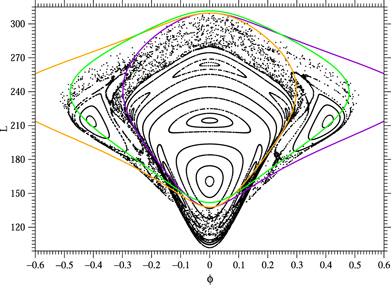
Figure 2. The Poincaré map restricted to the NHIM for E = −2650. The green curve is again the horizontal Lyapunov orbit which here no longer belongs to the NHIM. The orange and the violet curves are the two horizontal periodic orbits which have been split off from the horizontal Lyapunov orbit in its pitchfork bifurcation at E = −2678.
Download figure:
Standard image High-resolution imageWhen we increase the energy further then the decay process proceeds and the dwell time of trajectories in the region which has developed from the former chaotic region becomes smaller. Figure 3 shows the Poincaré map for the energy E = −2550. In black colour such structures are plotted which are still located in the surviving parts of the NHIM and have a permanent existence as parts of the invariant surface. They are the island around the central fixed point belonging to the vertical Lyapunov orbit and small inner parts of the islands around the tilted loop orbits. In addition a KAM curve in the largest surviving island chain inside of the chaotic region is plotted in black colour, this island chain belongs to a 1:7 resonance. The horizontal Lyapunov orbit is still included as a green curve, even though it is already rather far away from the remnants of the NIHM.

Figure 3. The Poincaré map restricted to the NHIM for E = −2550. The green curve is again the horizontal Lyapunov orbit. Structures on the permanent part of the remaining NHIM surface are plotted in black. Points on the transient remnants of the NHIM surface are plotted in light grey (for more details see the main text). Various parts of one transient trajectory are plotted in colour. The initial point is marked as a blue 8-pointed star. The blue circles are the sequence of iterates which still can be stabilized by a projection on the transient remnants of the stable manifold of the NHIM. The red 8-pointed star is the first iterate which can no longer be stabilized not even over the transient remnants of the NHIM. The red circles are further iterates.
Download figure:
Standard image High-resolution imageAlso included in figure 3 is a single trajectory which starts in the region which for smaller energy has belonged to the large chaotic region on the NHIM. That is, it starts in the transient tangential continuation to the outside of the central island. The initial point of the trajectory is marked as a blue 8-pointed star. For this trajectory we have applied the projection on the transient remnant of the stable manifold of the NHIM after each intersection with the surface z = 0, i.e. after the creation of each new point in the map. Thereby we can observe immediately when the trajectory leaves the region where a temporary stabilization of the trajectory is still possible. Those points of the trajectory (iterates of the initial point represented by the blue 8-pointed star), which still can be stabilized on the transient part of the NHIM surface by this procedure, are plotted as blue circles. They are 9 in number.
When we intent to stabilise the 10th iteration, the numerical method fails. This first point which cannot be stabilised on the former NHIM surface (on the transient tangential continuation of the surviving parts of the NHIM surface) is plotted as a red 8-pointed star. However, the trajectory has been continued without further projections and the next 31 intersection points with the plane z = 0 are plotted as red circles. This sequence of red points moves very slowly away on the former NHIM surface in tangential and also in normal direction.
Whereas in surviving parts of the NHIM the normal instability is still larger than the tangential instability, this relation turns into the contrary in decaying parts. Therefore we observe that the transient trajectories leave the decaying NHIM surface mainly in the tangential direction. There is no local branch of the stable manifold of the NHIM and also no local branch of its unstable manifold in a close neighbourhood of the red points. The 32nd iteration of the red 8-pointed star lies already outside of the frame of the figure.
Strictly speaking the whole coloured trajectory does not belong to the NHIM. However, the blue initial part of the trajectory is related to the NHIM at least in a transient sense. In this same sense we might consider the support of the blue points and the support of corresponding trajectory segments for other initial conditions as a transient remainder of the decaying NHIM surface. The corresponding trajectory segments for several other initial conditions have been included into the figure as light grey points. All such grey trajectory segments have only a transient meaning as trajectories associated with the NHIM. The transient part of the decaying NHIM consists of the union of small neighbourhoods of all the light grey points.
This transient dynamics stands in sharp contrast to the islands around the tangentially stable fixed points which are still truely invariant surfaces in the domain of the Poincaré map. In these true NHIM regions our combined development and projection method still produces any desired number of iterates of any initial point.
If we increase the energy still further then the central island shrinks slowly while the tilted loop islands shrink quite fast and disappear for E → −2534. At this energy E = −2534 the tilted loop orbits themselves become normally parabolic, disappear in bifurcations and thereby they are lost from the NHIM. Then the remnant of the NHIM consists of a moderate size neighbourhood around the central fixed point only.
3.2. Dwell time behaviour near the NHIM
Now we show an illustrative example how the search for the intersection between the line C of initial conditions and  is successful as long as we search in the still existing parts of the NHIM and becomes problematic in regions where the NHIM is already in the process of decay. As before, we choose a neighbourhood U of the NHIM, and define a line segment C, in our present example we choose for C a line segment pointing into the px
direction. We place 401 evenly distributed initial points pj
along C and calculate for each one of these points the number of intersection points with the plane z = 0, i.e. the number of iterations in the restricted map, before the trajectory leaves the region U. That is, we use the iteration number in the map as a discrete time measure. Thereby to each point pj
on C we obtain an integer valued time tj
which represents the dwell time of this trajectory in the neighbourhood U. The figure 4 shows graphically the result for 2 different initial line segments. The plot displays tj
as function of j. For a better guidance of the eye we have plotted a continuous curve, even though only integer values of j are used. We still use the energy value E = −2550.
is successful as long as we search in the still existing parts of the NHIM and becomes problematic in regions where the NHIM is already in the process of decay. As before, we choose a neighbourhood U of the NHIM, and define a line segment C, in our present example we choose for C a line segment pointing into the px
direction. We place 401 evenly distributed initial points pj
along C and calculate for each one of these points the number of intersection points with the plane z = 0, i.e. the number of iterations in the restricted map, before the trajectory leaves the region U. That is, we use the iteration number in the map as a discrete time measure. Thereby to each point pj
on C we obtain an integer valued time tj
which represents the dwell time of this trajectory in the neighbourhood U. The figure 4 shows graphically the result for 2 different initial line segments. The plot displays tj
as function of j. For a better guidance of the eye we have plotted a continuous curve, even though only integer values of j are used. We still use the energy value E = −2550.
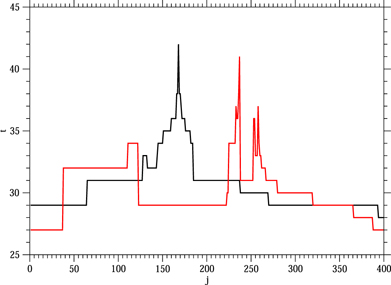
Figure 4. The number tj of iterated points under the restricted map which still lie inside of the neighbourhood U for 401 points pj along a line in px direction for 2 different values of the other initial coordinates. The exact values of the initial coordinates are given in the main text. For a better guidance of the eye continuous curves are drawn even though only integer values of j are used. The black curve belongs to an initial region where the NHIM still exists, the red curve belongs to an initial region where the NHIM has left behind transient remnants only.
Download figure:
Standard image High-resolution image
First we choose a line of initial points in a region where the NHIM still exists. Along this line the coordinates x = 4.165 19, y = −0.000 93, py = 59.193 43 are fixed and in px direction the interval [0.004 76, 0.004 78] is selected. The corresponding central initial point has the polar coordinates ϕ = 0, L = 246.55, in the figure 3 it belongs to the KAM curve of the 1:7 resonance island. This island chain is still a stable part of the NHIM even though it lies in the large decaying chaos region.
The resulting function tj
is the black curve in the plot of figure 4. Here the region of the maximal values of tj
is evident at first sight, it lies around the j value 168 having the t value 42. To both sides the values of tj
diminish rapidly if the index j moves away from the peak position. It is also clear in which region we must zoom in, if we want a better resolution of the intersection with  .
.
After a zoom the curve looks very similar, only the values of t become higher. If we increase the resolution along the initial line by a factor 100 then the values of t increase by 9. This indicates that the transverse instability (transverse eigenvalue) of the NHIM in the region under investigation lies in the order of magnitude of the 9th root of 100, i.e. around 1.7.
Next we choose a different line C, again pointing into the px direction, but this time in a region of the domain of the map, where the NHIM has a transient remnant only, it has the fixed coordinates x = 4.260 57, y = −0.177 39, py = 60.553 32 and the px coordinate comes from the interval [1.822 186, 1.822 191]. The central initial point has the polar coordinates ϕ = −0.04, L = 258.3, in figure 3 it is the 9th point of the blue trajectory (the last one of this trajectory which could be stabilised on the transient remnants of the NHIM) and it lies in the light grey region where the NHIM is already in the process of decay.
The resulting values of tj as function of j are plotted as the red curve in figure 4. Now we do not have a clear single maximum of the time values, in the region of large time values there are various jumps up and down. But we can at least see in which region of px values we should magnify in order to search for even higher values of tj . This indicates that in this region there exists only a kind of transient remnant of a stable manifold belonging to the transient remnants of the NHIM. In addition, in this case we do not see a clear rule for the increase of the maximal tj as function of the resolution along the line of initial conditions when we zoom in around some high values of pj .
When we move further away from the remaining parts of the NHIM then the dwell time along the line C of initial conditions develops more and more jumps up and down but jumps with smaller hight. Therefore it becomes less and less clear what the relevant maximum should be. In this way the transient behaviour slowly fades out. Accordingly, we cannot define a clear cut outer boundary of the region where transient remnants of the NHIM still have a significant influence. Of course, if we use a sufficiently large curve C of initial conditions then this line will almost always intersect  of the remainders of the NHIM somewhere far away from the initial point we are really interested in. However, this cannot be taken as an intersection with
  close to the initial point.
These two examples are representative and illustrate how numerically surviving parts of the NHIM and transient remnants are distinguished. Unfortunately, so far no clear behaviour of the statistics of the dwell time over transient remnants of the NHIM is evident from our study of many transient trajectories. Also no clear scaling behaviour is visible. More on this problem will be said in the final remarks in the next section. Finally the following observation is important: even though the exact values of tj depend on our choice of the region U, the qualitative properties of the function tj do not.
4. Conclusions and final remarks
In this article we point out a type of transient behaviour which to our knowledge has not yet been discussed before. It is the finite time trapping of a trajectory on a decaying lower dimensional invariant surface.
Maybe the reader has expected a more quantitative description of the transient chaos encountered. Unfortunately this was not possible because of the following reasons: the usual measures of chaos can be calculated best by the thermodynamical formalism [24, 25]. This formalism (and other ones equally) and also the mathematical definitions of these measures are based on a hierarchical structure of the chaotic set and on an (at least approximate) exponential scaling behaviour of this hierarchy. And this exponential behaviour is based on (at least approximate) hyperbolicity of the chaotic invariant set. If nonhyperbolicities only occur on high levels of the fractal hierarchy, then we can evaluate low levels only and obtain good approximations for the measures of the chaos.
However, in our case we are far away from hyperbolicity. The chaotic region of the NHIM is dominated by the complicated fractal distribution of small surviving KAM islands which cause enormous stickiness for general trajectories in their neighbourhood. Then nonhyperbolicity dominates already the low levels of the hierarchy. Let us quote a sad conclusion given in section 15.6 of [25]. Here comes a verbatim quotation (page 175 in the paperback reprint from 1997): 'Most rigorous results of the thermodynamical formalism can only be proved for hyperbolic systems. On the other hand, generic nonlinear maps appear to be nonhyperbolic. The situation here is no different from that in other fields of physics: most systems of real interest do not fit the conditions necessary for a rigorous treatment'. Unfortunately this conclusion applies fully to our present systems and therefore we have been forced to restrict the treatment to a qualitative one and to rely heavily on topological considerations.
As we see in the figures 2 and 3, the remaining parts of the NHIMs are dominated by regular behaviour and the large scale chaotic regions are the ones which already are in the process of decay. Now the reader may ask whether this result is exceptional for this particular system or whether it is typical.
First, numerical experience with various examples shows that it seems to be typical. Let us quote a few examples where 2-dimensional NHIMs in 4-dimensional maps form large scale chaotic regions near the boundary of decay: the figure 7 in [13] shows the decay scenario of an NHIM in a model map. The figure 4 in [26] shows the perturbation scenario of the NHIM for an electron in a perturbed magnetic dipole field. Here the perturbation consists in the addition of quadrupole components to the magnetic field. The figures 12 and 13 in [27] show a similar behaviour in a model for an open star cluster in the tidal field of a galaxy. The figures 16–19 in [28] show the decay scenario of two different not symmetry related NHIMs in a model for two interacting dwarf galaxies. And finally the figures 14 and 15 in [29] show a similar decay scenario for two different NHIMs in a model for a double-barred galaxy. In all the astronomical examples the energy is the perturbation parameter. So we see again and again the same phenomenon in quite distinct examples.
However, we also found a counter example. In [30] we studied a system where the NHIM starts to decay without the previous formation of any large scale chaotic region. This example is the hydrogen atom in a rotating external electric field. Also here the energy plays the role of the perturbation parameter. So the conclusion is, that the scenario of the present example is not generic in the strict mathematical sense, but it seems to be common.
To understand better the frequency and the repetition of the same qualitative scenario, the following general consideration might be helpful. At the beginning of the scenario, i.e. near the energy ES the internal dynamics of the NHIM is described well by the quadratic approximation of the effective potential. And then it is obvious that the internal dynamics is integrable, it is the one of an anisotropic harmonic oscillator. Chaos on a large scale in the internal dynamics can appear only, when the perturbation becomes large. Internal chaos and the decay both require an appreciable tangential instability. Therefore it is no surprize that the formation of large scale chaotic regions also indicates the tendency towards the beginning of the decay. Interestingly the reverse is not always true, as the above mentioned counter example [30] shows.
There is the related question of the robustness of the scenario described. Under small perturbations the internal dynamics of an NHIM shows small changes. Therefore this internal dynamics is not structurally stable in the strict mathematical sense. However, the qualitative structure of the NHIM is conserved. What changes can we expect under the inclusion of small additions to the potential? First, the shape of the invariant surface may be deformed slightly and the exact position of the NHIM in the domain of the map may be shifted. Second, the normal and the tangential instability at each individual point of the NHIM surface can be changed. As a consequence of this change of eigenvalues, the exact value of the energy may shift, at which the decay of the NHIM starts. And the exact front of the decay of the NHIM surface for a particular energy value may be shifted. However, these are only changes of tiny details of the scenario which do not imply changes of the overall picture.
Therefore in section 2 the description of the scenario has intentionally been kept on a qualitative level. We expect that this qualitative description of the tangential transient behaviour applies to all systems with a qualitatively similar development scenario. In the mathematical literature the expression 'persistence' is used for the qualitative robustness properties of NHIMs.
We have focussed on the case of codimension-2 NHIMs in 3-dof systems. Finally we have to consider whether these values of the dimensions are essential for the kind of transient behaviour described in this article and what happens for other values of the dimensions. For 2-dof systems the only type of NHIMs are hyperbolic periodic orbits and they do not have any internal dynamics at all. Here the whole unstable invariant subset disappears at one critical value of the perturbation. But it leaves behind a transient trapping effect in a region around the position where the periodic orbit has disappeared. This behaviour is essential for the phenomenon of intermittency, see section 4.4 in [22]. For systems with 4 or more dof, let us say n-dof, we can have NHIMs of various dimensions. In the map the dimension of the various NHIMs can be any even number from 0 to 2n − 4.
Let us have a fresh look at figures 1–3. They represent the internal dynamics of the NHIM and they are Poincaré maps for a 2-dof dynamics. In such a map the KAM lines, for example the ones in the islands around the stable fixed points, are impenetrable curves for the restricted map. Therefore trajectories starting exactly on the NHIM surface and inside of the outermost KAM curve of an island can never diffuse out into the chaos region around this island by motion restricted to the NHIM surface. This also holds for initial points in fine chaos strips in the interior of the islands. The same argument also holds for NHIMs of dimension 2 in maps of a higher dimension, i.e. systems with a higher number of dofs.
The situation is different for invariant surfaces of dimension 4 or higher in the map. Here the internal dynamics of the NHIM has 3 or more dof and then Arnold diffusion comes into play. In this case also trajectories starting in small chaotic stripes inside of islands can diffuse out of the island and can in the long run diffuse into regions of the NHIM which are already in the process of decay. Of course, then lower dimensional parts of the island still may be invariant, but these parts are no longer smooth surfaces of the full dimension of the former NHIM. Therefore, for higher dimensions of the NHIM we expect the transient nature of trajectories to appear in chaotic regions distributed all over the whole NHIM. And this transient behaviour can start as soon as the NHIM starts to decay somewhere.
In any case the transient behaviour starts in chaotic regions and thereby also the transient dynamics is chaotic. In this sense we have a new version of transient chaos. In the present article we have concentrated on Hamiltonian systems. Analogous phenomena should also be possible around decaying NHIMs in dissipative systems.
Data availability statement
All data that support the findings of this study are included within the article (and any supplementary information files).
Acknowledgements
The author thanks DGAPA for financial support under Grant number IG-100819 and CONACyT for financial support under Grant number 425854.