
Abstract
In large buildings, linking heating, cooling or ventilation systems between themselves and to physical spaces is a very time-consuming task that requires highly skilled engineering knowledge, as all these systems are interconnected and they have a certain influence to each other (ventilation systems are often connected to heating and cooling), which often makes task of locating the sources of error or anomalies very time consuming and difficult as they are performed manually. A different approach would be to work out relationships and equipment linkage from time series data provided by the sensors, thus inferring equipment links from which anomalies can be traced back to the source more easily. This paper proposes a data-based solution to obtain equipment relationships based on cross-correlations to relate Air Handling Units (AHUs) to their respective areas of operation. We also propose a methodology, in particular for AHUs, to identify whether or not to trust correlations based on the difference between supply and return temperature. A case study is presented based a large building with 16 AHU systems.
Export citation and abstract BibTeX RIS

Original content from this work may be used under the terms of the Creative Commons Attribution 4.0 licence. Any further distribution of this work must maintain attribution to the author(s) and the title of the work, journal citation and DOI.
Nomenclature
| AHC | Agglomerative Hierarchical Clustering |
| AHU | Air Handling Unit |
| ANN | Artificial Neural-Network |
| APAR | Air Handling Unit Performance Assessment Rules |
| BMS | Building Management System |
| DTW | Dynamic Time Warping |
| FCU | Fan Coil Unit |
| FDD | Fault Detection and Diagnosis |
| GRNN | General Regression Neural-Network |
| HVAC | Heating, Ventilation, and Air Conditioning |
| MTS | Multivariate Time Series |
| SAT | Supply Air Temperature |
1. Introduction
Building Management Systems (BMS) present clear advantages for energy control such as identifying locations of potential energy waste for energy optimisation, decreasing equipment operating cost, providing indoor environmental safety and comfort through Heating, Ventilation, and Air Conditioning (HVAC) systems control, as well as controls of water consumption, elevators, etc. Over the past few years, a lot of efforts have been put to control the three main important aspects of the building: energy consumption, security and comfort. The schematic in figure 1 represents the a high level overview of the built environment and role of BMS control signals and information flow, which also takes into account the supply of energy and data from the grid for demand response events. This figure shows the main building blocks of BMSs, in relation to the whole smart building spectrum:
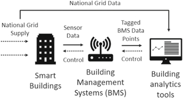
Figure 1. Schematic of BMS.
Download figure:
Standard image High-resolution imageThis paper is focused on BMS linkage, which is mainly used for the purpose of failure detection. The first two experiments are focused on AHU supply and return temperatures with sensor data from physical spaces. The physical spaces for these two experiments correspond to the manufacturing part facility in the ground floor. The last experiment is slightly different, as supply and return temperatures from AHUs are linked with fan coil units, which at the same time feed air to a different part of the facility: the office area in the first floor.
The literature has been reviewed in two main parts: the first one is dedicated to supervised and unsupervised HVAC equipment linkage for fault detection and diagnosis, as the main purpose of linking HVAC equipment is to trace back system failures and to detect system anomalies. The second one to time series clustering, as these are the kind of methodologies that we use to solve this problem.
When mobilising a set of building sensors into an analytics platform, BMS points are translated into a naming standard such as Haystack [1] or a more unified metadata schema such as Brick [2], so that the analytics platform can recognise them, and sensor points can be programmed into rules for energy consumption, systems linkage, etc which requires a metadata framework to form a link between point types, physical spaces and the linkage of HVAC components with the purpose of building knowledge relationships. One of these methods is the framework for metadata normalisation Plaster in [3], which requires a certain level of human supervision such as knowing the point type, location and relationship with other equipment parts, specially in large facilities. A methodology that works out relationships between HVAC points based on sensor data may help to reduce human interaction when building this framework.
Ventilation is one of the major areas of electricity consumption. In large industrial facilities, Air Handling Units (AHUs) are key consumption points. As represented in figure 2, several units are also involved in AHUs, such as electric fans, humidifiers (in some AHUs), heating and cooling, which interact with other systems, such as boilers, cooling systems, etc. Therefore, controlling AHU's parameters means to control a significant part of electricity consumption, as this is a point where other systems converge. The goal of this paper is to infer relationships between AHUs and both building areas and other HVAC parts for large manufacturing facilities using only time series data.
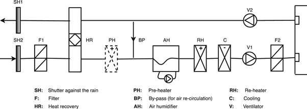
Figure 2. Schematic of AHU.
Download figure:
Standard image High-resolution imageOther studies have presented novel methodologies to infer relationships between HVAC components of large commercial buildings such as [4], that utilises perturbations of subsystem variables to reveal correct associations with a 76% success. The authors state that statistical methods are not good for this problem, however they only use correlations between variables and they don't test more complex statistical related methodologies. [5] uses a series of supervised learning methodologies to infer point type from sensor data, as well as to control perturbations to verify relationships between HVAC system parts [6]. Studies a comparison between different supervised learning methodologies, inferring equipment characteristics from time series features. The case study presented in our paper proposes a system with old infrastructures where no documentation nor prior knowledge is available, therefore a supervised learning classification approach would not be of use. Inputs and outputs are known but, in order to verify such outputs, verification from experienced engineers has been necessary in order to compensate the lack of documentation, which has been a work that lasted several weeks. Similarly, [7] uses supervised classification to infer AHU-VAV links by first extracting statistical features from the data and then random forests for each VAV. A study offering relationship between equipment parts according to physical spaces and with minimal intervention is presented in [8], which converts time series into frequency domain with short-time Fourier transformation operator, that contains implicit information about changes. Then it wraps them in time dimension by using dynamic time warping and a pre-defined time wrapping function.
As a part of this study, we consider that the methodology applied could be useful for diagnosis of system errors, which are defined after establishing normal working conditions of the system according to the clusters. When there is a significant number of AHUs and the temperature gets outside a comfort policy, the origin of this failure can be very difficult to trace back. For AHU fault diagnosis some previous work has been reported in the literature [9]. Describes the application of Artificial Neural Networks (ANNs) to the problem of fault diagnosis in an AHU by using residuals of system variables to quantify the dominant symptoms of fault modes of operation. Following the same approach, [10] proposed AHU subsystem level fault detection using a General Regression Neural-Network (GRNN), residual generation and fault detection and diagnosis. A novel feature extraction technique to extract temperature and power associated features from high-dimensional and unstructured terminal unit data is presented in [11], to diagnose faulty HVAC in an automatic and remote manner. The use of Air handling unit Performance Assessment Rules (APAR) was exercised by [12]. They use control signals to determine the mode of operation of the AHU. A subset of expert rules which correspond to that mode is then evaluated to determine whether a fault exists. In the review of fault detection and diagnosis methodologies carried by [13], various Fault Detection and Diagnosis (FDD) are described to illustrate the use of evaluation standard parameters for improving the performance of AHUs. This work divides FDDs in three main categories, namely analytical-based methods, knowledge-based methods, and data-driven methods. In a more recent study, [14] proposes a method that employs sequential two-state clustering to identify abnormal behaviour of the fan coil unit. Some other recent studies on HVAC systems fault detection and diagnosis can be seen in [11, 15, 16].
The methodologies for detecting failures of AHUs have the specificity of using either control signals or the internal parameters of the AHU itself. In large facilities, we link different physical spaces with their correspondent control systems to detect the sources of deviation from the prescribed conditions. There is growing need of understanding and extracting value from sensor data, specially in large spaces where the amount of AHUs and of time series data provided by the different sensors can create confusion when looking for links between different equipment units. So the real problem we aim to solve is to add clarity about equipment-spaces linkage and therefore, to create real value from sensor data.
This sensor data linkage is done by studying similarities between the time series data, and by clustering them based on these similarities [17]. States that finding the clusters of time series can be advantageous in different domains for anomaly, discord detection, recognising dynamic changes in time series, prediction and recommendation and pattern discovery. The problem we study fits into the pattern detection category, as we aim to detect similarities between time series to identify links between assets.
One of the widely used metrics for time series similarities is Dynamic Time Warping (DTW). One of the pioneer works, [18] describes experiments with this dynamic programming approach to the problem of pattern detection [19]. Demonstrates that DTW could be used for mining massive data sets faster than with euclidean distance [20]. Designs an approach that penalizes points with higher difference between a reference point and a testing point in order to prevent minimum distance caused by outliers.
Some other distance metrics have proven successful for pattern detection in time series data. Integrated periodogram distance [21] presents a metric based on different dependence measures to classify time series as stationary or non-stationary. Simulations results proved that the logarithm of the normalized periodogram and the metric based on the autocorrelation coefficients can all distinguish ARMA and ARIMA models, which does not happen with the classical Euclidean distance. Lasso-based approaches are also widely used for time series grouping. As an example, [22] proposed a two-step Lasso procedure for multiple change-point estimation in time series. [23] used LASSO-Patternsearch algorithm for detecting disease-causing genes. [24] decompose high dimension multivariate time series (MTS) into smaller dimension MTS which are relatively independent of one another, based on correlation between the variables.
In recent years, several studies have been done in the field of time series clustering, such as [25], which presents a time series clustering approach for building automation and control systems. This work uses unsupervised machine learning algorithms to improve supervised classification by adding more robust features compared to manual selection [26]. Compares a set of recurrent neural networks on groups of similar time series for clustering, showing that long-short-term memory neural networks present a good result for this purpose as well. Other recent works on time series clustering methodologies and applications can be seen in [27, 28].
In this paper, we apply clustering techniques to relate Air Handling Units (AHUs) to their respective areas of operation. In section 2 we explain the methodology, and introduce methods and similarity measures. In section 3 we describe the data of this case study and introduce the concept of difference in temperature for testing hypothesis. Later in section 4 we design the experiments. Finally, we present the conclusions in section 5.
2. Mehodology
The goal is to partition a set of data objects into homogeneous groups or clusters using machine learning techniques, in order to group similar sensor time series together depending on which of the three experiments. Partition is performed in such a way that objects in the same cluster are more similar to each other than to objects in other clusters. We make this differentiation with correlations. In this work, several time series data clustering metrics are tested, namely correlations, dynamic time warping and integrate periodgram distance. We use these metrics to perform agglomerative hierarchical clustering and then we test a different clustering methodology: Graphical Lasso.
2.1. Graphical Lasso
In [29], the problem of estimating sparse graphs, graphs with only few edges, by a lasso penalty to the inverse covariance matrix is considered. Let us consider the case where X1, ..., Xn are independent and identically distributed Np (μ, Σ) and being the estimated precision matrix, which is the inverse matrix from the covariance matrix, denoted Ω ≡ Σ−1. This function solves the following optimisation problem:

where tr is the trace, λ > 0 and the penalisation parameter  is the L1-Norm of Σ (Lasso regularisation parameter). In order to provide useful information, this problem proposes to maximise the penalized log likelihood with respect to Ω, so the nodes are not fully connected and the connections kept on each cluster have useful information concerning the relationships of time series on each cluster. This happens because Lasso regularisation parameter shrinks the less important features coefficient to zero, removing less meaningful coefficients. The algorithm employed to solve this problem is the GLasso algorithm, which is explained in [29], where they consider the problem of estimating sparse graphs by a lasso penalty, which is the penalty applied to non-zero coefficients by the sum of their absolute values, applied to the inverse covariance matrix.
With this estimate of the inverse of the correlation matrix, we have the partial independence relationship. If two features are independent conditionally on the others, the corresponding coefficient in the inverse of the covariance matrix would be zero, as it learns independence relations from the data, instead of being a distance measure itself between time series.
According to the authors of the implementation package in 'scikit-learn' in [30], the search for the optimal penalization parameter is done on an iteratively refined grid: first the cross-validated scores on a grid are computed, then a new refined grid is centred around the maximum, and so on. One of the challenges here is that the solvers can fail to converge to a well-conditioned estimate. The corresponding values of alpha then come out as missing values, but the optimum may be close to these missing values.
2.2. Agglomerative hierarchical clustering
Agglomerative Hierarchical Clustering (AHC), has a long history, especially in taxonomy or classificatory systems, and phylogenetics [31, 32]. Further studies generalised this algorithm, [33], and have further developed and improved [34, 35].
Base on the definition given in [36], the goal of hierarchical clustering is to create a sequence of nested partitions or clusters, which can be conveniently visualised via a tree or hierarchy of clusters, also called the cluster dendrogram. In AHC, it starts with each of the n points in a separate cluster, and then merging the two closest clusters until all points are members of the same cluster. Algorithm 1 shows this procedure, with  , where
  , a clustering ζ = {C1, ..., Ck
} is a partition of
, a clustering ζ = {C1, ..., Ck
} is a partition of  .
.
Algorithm 1. Agglomerative Hierarchical Clustering (D, k), reproduced with permission from [36]:
1  ; // Each time series is in a separate cluster initially
2  ; // Compute matrix with distances
3 repeat
4 Find the closest pair of clusters Ci
, Cj
∈ ζ ;
5  ; // Merge the clusters
6  ; // Update the clustering
7 Update distance matrix Δ to reflect new clustering;
8 until 
Different distance measures between time series can be used for clustering: pearson's correlation coefficient, dynamic time warping and integrated periodogram distance.
2.2.1. Pearson's correlation similarity
Let ![$x={[{x}_{1}{x}_{2}...{x}_{L}]}^{T}$](https://content.cld.iop.org/journals/2631-8695/2/4/045003/revision4/erxabbb85ieqn10.gif) and
and ![$y={[{y}_{1}{y}_{2}...{y}_{L}]}^{T}$](https://content.cld.iop.org/journals/2631-8695/2/4/045003/revision4/erxabbb85ieqn11.gif) be two zero-mean real-valued random vectors of length L. As described in [37], the Pearson's correlation coefficient between x and y is
be two zero-mean real-valued random vectors of length L. As described in [37], the Pearson's correlation coefficient between x and y is

With E being the expected value. According to the 'tsclust' package documentation in [38], which is the one used for the purpose of this study, two different measures of dissimilarity between two time series based on the estimated Pearson's correlation can be computed. These can be  or
or  , where β specifies the regulation of the convergence.
2.2.2. Dynamic Time Warping
DTW has the basic idea behind that the sequences are extended by repeating elements and the distance is calculated between extended sequences. Therefore, DTW can handle input sequences with different lengths [39].
Let ![$x={[{x}_{1}{x}_{2}...{x}_{r}]}^{T}$](https://content.cld.iop.org/journals/2631-8695/2/4/045003/revision4/erxabbb85ieqn14.gif) and
and ![$y={[{y}_{1}{y}_{2}...{y}_{s}]}^{T}$](https://content.cld.iop.org/journals/2631-8695/2/4/045003/revision4/erxabbb85ieqn15.gif) be two time series, where lengths r and s are not necessarily equal. Let M be an r × s matrix with the (i, j) element containing the squared Euclidean distance between two points xi
and yj
. Each element (i, j) in M corresponds to the alignment between two points xi
and yj
. Let
be two time series, where lengths r and s are not necessarily equal. Let M be an r × s matrix with the (i, j) element containing the squared Euclidean distance between two points xi
and yj
. Each element (i, j) in M corresponds to the alignment between two points xi
and yj
. Let  be a warping path, where the kth element wk
= (ik
, jk
). Then
be a warping path, where the kth element wk
= (ik
, jk
). Then  with the warping paths having the following restrictions: monotonicity, continuity and boundary conditions. There are exponentially many paths that satisfy these conditions, being the optimal path the one which minimizes the warping cost [40]:

where (il
, jl
) = wl
for l = 1, 2, ..., K. Then the optimal path can be found through dynamic programming according to  , where γ(i, j) is the dynamic time warping distance between the sub sequences x1, x2, ..., xi
and y1, y2, ..., yj
.
, where γ(i, j) is the dynamic time warping distance between the sub sequences x1, x2, ..., xi
and y1, y2, ..., yj
.
2.2.3. Integrated Periodogram Distance
The distance based on the normalised periodogram was introduced in [21]. Let  and
and  be periodograms of time series x and y, respectively, at frequencies
 ![${w}_{j}=2\pi j/n,j=1,\ldots ,[n/2]$](https://content.cld.iop.org/journals/2631-8695/2/4/045003/revision4/erxabbb85ieqn21.gif) in the range 0 to π, [n/2] being the largest integer less or equal to n/2. We are interested only on its correlation structure, so it is better to use normalized periodogram defined by
in the range 0 to π, [n/2] being the largest integer less or equal to n/2. We are interested only on its correlation structure, so it is better to use normalized periodogram defined by  , where
  is the sample variance of the time series. Also, since the variance of the periodogram ordinates is proportional to the spectrum value at the corresponding frequencies, logarithms can be taken and therefore, the distance between x and y can be defined by

Knowing that the periodogram has the equivalent representation ![$P({w}_{j})=2\left[{\hat{\gamma }}_{0}+{\displaystyle \sum }_{k=1}^{n-1}{\hat{\gamma }}_{k}{\cos }({w}_{j}k)\right]$](https://content.cld.iop.org/journals/2631-8695/2/4/045003/revision4/erxabbb85ieqn24.gif) , where
, where  is the sample autocovariance function (defined with more detail in [41]) which, according to the authors, leads to

2.3. Implementation
3. Problem and data description
The building used in this case study is a large manufacturing facility that consists mainly on manufacturing facilities in the ground floor (AHUvs physical spaces experiments 1 and 2), and office spaces inthe first floor (AHU vs FCU experiment 3).
3.1. Experiments 1 and 2: Manufacturing facility (Ground floor)
The manufacturing part is comprised of several spaces, every space dedicated to a part of the process, as this is an automotive manufacturing plant. In terms of cooling, heating and ventilation systems, the building has 3 chillers, 6 boilers, 6 fan coil units and 16 multi-speed fan AHUs. As the focus of this paper are AHU systems, the actual linkage between AHU-space and type can be seen below in table 1. Some of the AHUs have been discarded due to the lack of sensors in their respective areas of influence, which makes them irrelevant to this study.
Table 1. Ground truth of AHUs of the manufacturing facility for experiments 1 and 2, their associated areas of influence and the number of temperature sensors in such areas. AHUs' temperatures are controlled by the average value of the temperature sensors located in their respective areas, with a data resolution of 10 minutes.
| AHU | Associated zone | Control strategy | N. of temperature sensors in the zone |
|---|---|---|---|
| AHU01 | Lab rooms | Avg. room temp—Fixed set point | 4 |
| AHU02 | Support room | Avg. room temp—Fixed set point | 3 |
| AHU03 | Wax room | Avg. room temp—Fixed set point | 4 |
| AHU04 | Shell room | Avg. room temp—Fixed set point | 4 |
| AHU05 | NPI room | Avg. room temp—Fixed set point | 3 |
| AHU06 | Clean room | AHU Return temp—Fixed set point | 0 |
| AHU07A/7B | Foundry area | Avg. room temp—Fixed set point | 8 |
| AHU09/10 | Finish room | Avg. room temp—Fixed set point | 4 |
| AHU11 | Inspection/X-Ray rooms | PI control loop—variable set point | 5 |
| AHU12 | Canteen | Avg. room temp—Fixed set point | 1 |
| AHU14 | Pre-fire room | Avg. room temp—Fixed set point | 2 |
| AHU15 | Fresh air make-up unit | Fixed supply temp | 0 |
| AHU16 | Shell rooms | Avg. room temp—Fixed set point | 2 |
We based our experiments on ground truth table 1. The data has been extracted directly from the manufacturer for every AHU individually [43], technical specifications include also dimensions of boxes and specs. of motors, fans, thermal wheel (if applicable), coils, etc. The data set comprises BMS sensor records. Every sensor is tagged with a specific name describing the company and followed by building location and subset (Ventilation, Metering, Cooling, Heating, Globals, Terminals and Lighting).
The building used for this case study is a Rolls Royce plant located in Rotherham, with 1639 BMS points in total. The period chosen for this study is June to July 2018 (30 days). The facility comprises two main areas: the production plant on the ground floor and the offices in the upper floor.
Time series data provided by sensor points is not often reliable and there are data gaps to be filled, units to be removed, and anomalies, which are bits of data misplaced between points because of extraction. The used data points are:
- AHU Supply Air Temperature (SAT) points: These points measure the temperature of the air supplied to the area. There is one of these points per AHU.
- AHU Return Air Temperature (RAT) points: These points measure the temperature of the air extracted from the space prior to re-circulation or disposal.
- Room temperature points: Sensors are located in each room to measure temperature. There are between 1 and 4 sensors located on each room, and consists of averages of the sensors.
- Fan Coil Unit (FCU) room temperature: Output temperature of FCUs. This piece of equipment is connected (or close to) an AHU, and we define the relationships in one of the experiments below.
3.2. Experiment 3: Office spaces (First floor)
The office spaces contains the meeting rooms and common spaces such as restaurant, canteen, kitchen, changing room and open spaces. In this experiment we establish correlations-based relationships of these two types of equipment. This correlations study would illustrate the way in which different equipment types are linked, so the main influence areas are clearly defined. A schematic is shown in figure 3. In this case study building, FCUs feed air to specific meeting rooms in the office above the manufacturing facilities.
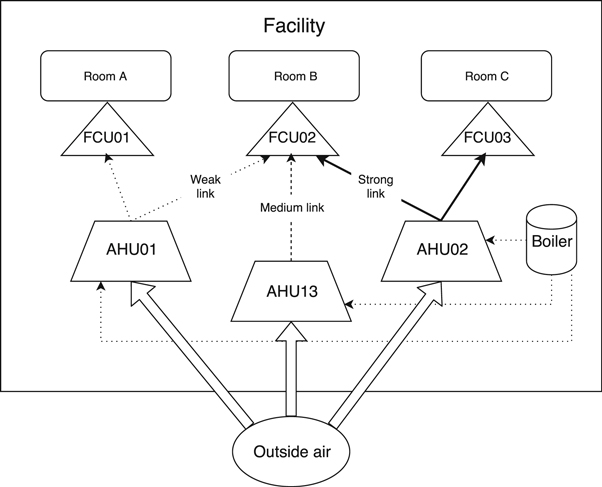
Figure 3. Schematic of AHUs and FCUs linkage.
Download figure:
Standard image High-resolution imageDifferent meeting rooms receive the following generic names: Rhenium, Tugsten, Nickel, Cobalt, Tantalum and the gym. The main goal of this experiment is to link the respective rooms, each being fed by a different FCU, with their closest AHU unit's area of influence, being the AHU's the same ones as in experiments 1 and 2.
4. Correlations experiments using real building sensor time series
We perform various experiments to relate AHUs with their respective work spaces, as well as FCUs with their respective AHUs. In experiment 1, we perform a comparison of the performance for different clustering techniques in a controlled experiment consisting of only a small part of the facility. Then the best performing methodologies from experiment 1 are used in experiment 2 for the whole facility. Experiment 3 shows a different clustering focus, linking a different piece of equipment, fan coil units, with their respective areas of influence.
4.1. Linkage significance and difference in temperature
In order to test if the correlations are reliable, we need to ensure their significance. If the link between room sensors and SAT is established, the internal difference in temperature is an important factor to take into consideration to define this significance. All spaces in the facility may generate heat internally (kitchen, manufacturing process, people, computer equipment, etc.) which could make difficult identification of spaces with their respective AHUs. This is why we measure this internal disruption in the first place, and then gradually add complexity to the clustering.
For this purpose, the difference between supply and return air temperature has been taken into account,

Table 2 represents the mean, variance, minimum and maximum value of the element-wise difference between supply and return air temperatures for each AHU.
Table 2. Mean, variance, minimum and maximum value of the difference between supply and return air temperature (Co ).
| AHU number | Mean | Variance | Min Value | Max Value |
|---|---|---|---|---|
| AHU01 | 2.39 | 7.25 | 0.00 | 11.30 |
| AHU02 | 6.20 | 14.37 | 0.01 | 13.45 |
| AHU03 | 8.01 | 0.90 | 0.48 | 14.62 |
| AHU04 | 2.87 | 0.97 | 0.02 | 8.47 |
| AHU05 | 3.74 | 0.63 | 0.04 | 10.89 |
| AHU06 | 3.97 | 0.75 | 0.06 | 6.20 |
| AHU07A | 17.16 | 1.06 | 12.92 | 20.18 |
| AHU07B | 15.49 | 1.13 | 12.28 | 18.34 |
| AHU09 | 10.37 | 1.40 | 8.23 | 14.86 |
| AHU10 | 10.12 | 1.59 | 6.69 | 13.80 |
| AHU11 | 2.28 | 0.98 | 0.00 | 4.99 |
| AHU12 | 3.50 | 5.50 | 0.00 | 10.69 |
| AHU14 | 8.09 | 17.38 | 0.00 | 15.61 |
| AHU16 | 1.04 | 0.56 | 0.00 | 7.90 |
Table 2 shows that some AHUs, such as 6, 7A, 7B, 9 and 10 present a much higher mean value of their difference in supply and return temperatures. However it can be seen that the variance in some of them is not very high, meaning that the high mean difference in temperature is stable. Probably one area has been constantly influenced by other areas. On the other hand we can find areas with a relatively low mean with a high variance, meaning that the physical space presents temperature disruptions very often. The reason to choose this value is that the clustering algorithms fail in linking AHUs with sensors above an approximate difference in temperature of 8 degrees Celsius in experiment 2.
These values are to be used as a measure on how much the defined AHU linkage can be trusted, therefore we decide to test the following hypothesis: we define a limit for the mean difference in temperature as 7.5, above which the cluster may not be reliable as the internal heat disruption may be too high so we are not able to ensure that the cluster is comprising these points is correct.
4.2. Experiment 1: Linking three AHUs to five different rooms
For the first experiment, three AHUs have been selected. We chose, according to table 2, the ones with a relatively low mean and variance thus, the ones with a lower internal difference in temperature. Also it is necessary to validate how good the solution is, so the site engineers are consulted on the room names to which the AHUs are supplying air to. The chosen AHUs and corresponding rooms are:
- AHU05 supplying air to the 'NPI room'
- AHU11 supplying air to the 'Visual inspection', 'Manual inspection' and 'X Ray' rooms
- AHU16 supplying air to the 'Shell drying' room
We apply the methodologies discussed to this first experiment and later we compare our results with the real connections. In a properly clustered group, the AHU's SAT should be in the same group together with their corresponding space temperature sensors. The dendrograms correspond to the AHC methodology with the three distance metrics. AHC can be represented as a dendrogram because the algorithm progressively separates the clusters based on the different distance metrics until all the points form a separate cluster. For this reason, the lasso clustering methodology is represented separately in table 3, as this algorithm does not respond to this type of representation because the search for the optimal penalisation parameter is done in an iteratively refined grid.
Table 3. Lasso clustering results
| AHU in cluster | Room temperature sensors in cluster | |
|---|---|---|
| Cluster 1: | AHU05 Supply Air Temp | Room NPI Room Temp No3 |
| Room NPI Room Temp No2 | ||
| Room NPI Room Temp No.1 | ||
| Cluster 2: | AHU16 Supply Air Temp | Drying Shell Drying Cell Temp No2 |
| Drying Shell Drying Cell Temp No1 | ||
| Cluster 3: | AHU11 Supply Air Temp | Room Manual Inspection Room Temp |
| Room Manual Inspection Room Temp.1 | ||
| Room Visual Inspection Room Temp | ||
| Room Visual Inspection Room Temp.1 | ||
| Ray X Ray Room Temp | ||
For the experiments, we assume that we know already that the BMS points belong to the different AHU systems and room temperature sensors. What we assume not to know beforehand are which of the 13 AHUs is associated with which of the 11 physical spaces. We know the parent-child relationship once the AHU has been associated with its corresponding physical space.
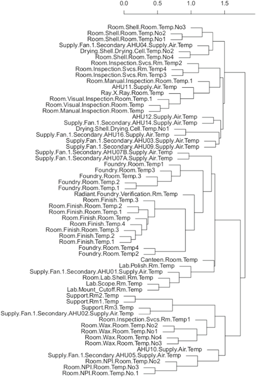
In the dendrograms, a distance between clusters has been chosen to the best convenience. The distance chosen determines which branches below that distance form a cluster. The same distances are used later in the experiment with the whole building evaluation. An ideal cluster should contain the AHU sensors together with their respective temperature sensors within the same. Figures 4–6 show the clustering results of the different distance metrics in the form of a dendrogram.

Figure 4. Experiment 1: Correlations based AHC with small subset of 3 AHUs. The number above indicates the incremental distance between clusters according to this metric.
Download figure:
Standard image High-resolution imageThe fact that the AHUs' SAT belongs in the same cluster as their respective room temperature sensors means in the case of AHC that, in the lowest levels of the dendrogram, the time series are closer (in terms of the chosen distance) to each other, and form groups that are more distant to each other as the branches go up. In the case of graphical lasso, it means that the elements corresponding to the estimated inverse of the covariance matrix are zero between groups of time series data or clusters, thus forming groups with the time series data that present the most similar number of common features.
Figure 4 shows that correlations-based AHC clusters AHU05 and AHU11 properly with their corresponding temperature sensors. AHU16 is in a cluster together with one of its sensors, however the other sensor is excluded, thus forming a separate cluster. Figure 5 shows the same clustering methodology but based on DTW. On this, it can be seen that the clusters do not respond to the logic of the physical connections, independently of the distance chosen to form the clusters. Similarly in figure 6 the clusters do not respond to the ideal behavior either. In table 3 we show the results of lasso clustering. In this case, the clusters respond to the most ideal behavior. The three AHUs are properly linked to their respective temperature sensors within the same cluster.

Figure 5. Experiment 1: Dynamic time warping based AHC with small subset of 3 AHUs. The number above indicates the incremental distance between clusters according to this metric.
Download figure:
Standard image High-resolution image
Figure 6. Experiment 1: Integrated periodogram distance based AHC with small subset of 3 AHUs. The number above indicates the incremental distance between clusters according to this metric.
Download figure:
Standard image High-resolution imageResults have been summarised in table 4. The percentages are obtained based on the rate of room temperature sensors contained within the cluster with their corresponding AHU each. For instance, correlations AHC clusters elements properly within AHUs 05 and 11 but missed one of the two elements in cluster containing AHU16. The one showing the best results is the graphical lasso clustering, properly grouping AHUs with their respective areas of influence. This performance is followed by correlations clustering.
Table 4. Distance between cluster chosen for each AHC metrics and success rate for both lasso and AHC.
| Clustering methodology | Hierarchical clustering | Lasso | ||
|---|---|---|---|---|
| Distance metrics | Correlations | DTW | IPD | — |
| Clusters distance limit | 1.4 | 10 000 | 150 | — |
| AHU 05 | 3/3 (100%) | 0/3 (0%) | 0/3 (0%) | 3/3 (100%) |
| AHU 11 | 5/5 (100%) | 0/5 (0%) | 1/5 (20%) | 5/5 (100%) |
| AHU 16 | 1/2 (50%) | 2/2 (100%) | 0/2 (0%) | 2/2 (100%) |
| % sucess sensors | 90% | 20% | 10% | 100% |
Now that the methodologies that perform best have been proved, we are proceeding with them both for the next experiment.
4.3. Experiment 2: Linking all AHUs to rooms (whole building evaluation)
In experiment 2, we use the two best performing methodologies discussed in section 4.2, Pearson's distance-based AHC and lasso clustering, with all AHUs and all temperature sensors within the building. We can see the dendrogram as a result of Pearson's correlation distance-based AHC figure A1, and the results for lasso clustering in table A1 in the appendix. In the results of the Pearson's correlation distance-based AHC shown in figure A1. Correct clusters are considered by using the same distance to analyse the clusters as in experiment 1. As an example for correct cluster, figure A1 shows that AHU01 is contained within the same branch levels as the four lab rooms, as expected. Similarly, AHU07A and AHU07B are clustered with the Foundry area. Other areas such as Finish rooms, Wax rooms and the canteen, they are in different clusters with respect to their AHUs. Interestingly, we observe that the related rooms are usually found together in the lowest level of the branches. Another observation is that AHUs that share common spaces are also clustered together, such as AHU07A and AHU07B. In the results of lasso clustering in table A1, as in experiment 1, we used two columns to separate AHUs and room temperature sensors within the same cluster. Some of the clusters only group room temperature sensors, but no AHU SAT is present, as is the case of clusters 2, 5 and 9. On the other hand, clusters with only AHUs and no temperature sensors are observed in cluster 11. AHU06 is discarded for the lack of sensors in the room.
As defined in section 4.1, we set a limit value of 7.5 for the difference between SAT and RAT. Below in table 5 we summarised the results obtained. The table describes the result, the average difference in temperature, confirmation/denial of linkage successful in the appropriate category and the issue associated with the AHU if applicable.
- Issue (a): Open plan space. Heat exchange occurring between nearby rooms.
- Issue (b): The AHU is enabled and demand is 100% cooling near constantly but is having no effect on setpoint (the temperature value set) or is not enough to cool to the set-point. This implies the AHU is not mechanically sound or capable to meet requirements but onsite investigation would confirm this.
Table 5. Summarised results of experiment 2.
| AHU | Mean ΔT | Associated room | Success rate AHC (Correlations) | Success rate Graphical lasso | Reported issue |
|---|---|---|---|---|---|
| AHU01 | 2.39 | Lab rooms | 4/4 (100%) | 4/4 (100%) | N/A |
| AHU02 | 6.20 | Support room | 3/3 (100%) | 3/3 (100%) | N/A |
| AHU03 | 8.01 | Wax room | 0/4 (0%) | 4/4 (100%) | N/A |
| AHU04 | 2.87 | Shell room | 4/4 (100%) | 0/4 (0%) | N/A |
| AHU05 | 3.74 | NPI room | 3/3 (100%) | 3/3 (100%) | N/A |
| AHU07A/AHU07B | 17.16/15.49 | Foundry area | 8/8 (100%) | 1/8 (12.5%) | (a) |
| AHU09/AHU10 | 10.37/10.12 | Finish room | 0/4 (0%) | 0/4 (0%) | (b) |
| AHU11 | 2.28 | Inspection/x-ray rooms | 5/5 (100%) | 5/5 (100%) | N/A |
| AHU12 | 3.50 | Canteen | 0/1 (0%) | 0/1 (0%) | (b) |
| AHU14 | 8.09 | Pre-fire room | 0/2 (0%) | 0/2 (0%) | N/A |
| AHU16 | 1.04 | Drying rooms | 1/2 (50%) | 1/2 (50%) | N/A |
| % Sensors clustered correctly | 70% | 52.5% | |||
Table 5 shows the results of this experiment. The performance of both methodologies is very similar, except that lasso fails to cluster wax rooms with their respective temperature sensors. In general, we can say that correlations based AHC performs better than graphical lasso in terms of number of sensors belonging to the correct cluster. 70% reveals that this methodology discovers underlying physical patterns between AHUs and their respective spaces. Also, it can be observed that the AHUs with a mean ΔT above the set-up limit fail to predict the matches between AHUs and physical spaces in general, although exceptions can be seen in graphical lasso and AHU03. AHUs 07 A and B are in the same branch as their respective sensors in the AHC technique. AHUs 2 and 12 have a very high variance (as shown in table 2), which does not seem to affect the performance of the algorithms in the case of AHU 2. For AHU 12, both methods fail to predict its only sensor with the canteen. When looking at its variance, it seems to be higher than other AHUs, as the canteen is crowded mainly during lunch time. This, together with the fact that its only sensor may be misplaced, could explain this issue.
We wanted to test the hypothesis of the difference in temperature having a determinant effect on obtaining these relationships. In the case of AHU07 A & B and despite being an open space, correlations-based AHC has been able to properly identify all 8 sensors in this more challenging case. Therefore we conclude this hypothesis cannot be confirmed or the experiment is insufficient.
4.4. Experiment 3: Linking AHU with Fan Coil Units (FCUs)
The main goal of this experiment is to link the respective rooms, each being fed by a different FCU, with their closest AHU unit. The strength of these links has been defined by the Person's correlation coefficient, with high showing a strong, very likely correlation, medium showing a moderate strength and low a weak link. These relationships are shown per FCU, and the links of these with all (if any) of the correlated AHUs. This is summarised in table 6.
Table 6. AHU and FCUs linkage. Numerical association with correlation and the degree of stregth defined by flag category.
| AHU | FCU Linked | Pearson's correlation coefficient | Linkage |
|---|---|---|---|
| AHU01 | Nickel | 0.68 | Medium |
| Tugsten | 0.34 | Low | |
| Gym | 0.29 | Low | |
| AHU02 | Nickel | 0.89 | High |
| Cobalt | 0.51 | Medium | |
| Tugsten | 0.51 | Medium | |
| Rhenium | 0.48 | Medium | |
| Tantalum | 0.05 | Low | |
| AHU04 | Cobalt | 0.14 | Low |
| Nickel | 0.11 | Low | |
| AHU07A | Tugsten | 0.25 | Low |
| Nickel | 0.24 | Low | |
| Gym | 0.06 | Low | |
| AHU07B | Nickel | 0.20 | Low |
| Tugsten | 0.14 | Low | |
| Gym | 0.06 | Low | |
| AHU09 | Nickel | 0.02 | Low |
| Gym | 0.01 | Low | |
| AHU10 | Nickel | 0.07 | Low |
| Tugsten | 0.04 | Low | |
| Gym | 0.02 | Low | |
| AHU11 | Cobalt | 0.06 | Low |
| Rhenium | 0.02 | Low | |
| AHU13 | Cobalt | 0.55 | Medium |
| Rhenium | 0.45 | Medium | |
| Tantalum | 0.16 | Low | |
| AHU16 | Cobalt | 0.08 | Low |
| Tantalum | 0.03 | Low | |
| Rhenium | 0.02 | Low | |
We conclude from correlations that the most influential AHUs to the FCUs are AHU 01, 02 and 13. Without having information about the equipment links, we have some degree of confidence to discard low-flagged category AHUs. After validation with the engineers, we found out that AHU02 is the one that has the highest influence over these areas. Therefore, we uncovered some other potential dependencies from the supply air temperatures of AHUs 01 and 13 to some of the rooms (Nickel, Tugsten and Gym for AHU01 and Cobalt, Rhenium and Tantalum for AHU13).
5. Conclusions
In this paper, we propose a solution to obtain equipment relationships based on data correlations and clustering that relate AHUs to their respective areas of operation. This is an important industrial challenge that requires a smart solution.
Graphical lasso and correlations-based AHC are the two best performing techniques in the first three experiments. In the first experiment, lasso clustering proved slightly better than correlations distance-based AHC. In the second experiment, however, their performance is quite similar, with few differences on Wax and Shell rooms but with the same number of successfully clustered elements. Experiment 3 shows satisfactory results as the physical spaces linked to the FCUs correspond with the real case. This approach allows to quickly scan the system, as one AHU can be connected to more than one FCU, being in the same area of influence in the case they are not directly attached.
This methodology can be generalised to large buildings with a similar problem. The system could potentially input labeled time series data corresponding to sensors and output the clusters. Although the accuracy is not 100%, this data-driven approach removes weeks of engineering visits to the facility to establish these relationships by hand and looking at the documentation. By applying this methodology, it becomes quite straightforward to establish a first step towards more advanced analytics or to determine a standard naming system that encompasses parent-child relationships.
This top-down perspective aims not to use internal parameters of AHUs and other BMS information, but instead their direct output. Systems internal information is less likely to be available in comparison to the room temperature sensors which are commonly installed, but the hardware connections are not documented. The most recent evolution in smart buildings implies the installation of a significant amount of sensors in large facilities, so this creates the necessity of generating real value from the data through data mining. Time series clustering can be used on a daily basis by the site engineers who need to trace back faults without the need of an extensive installation information on that particular building.
Acknowledgments
We would like to thank Tony Carter, for his vast knowledge in AHUs, HVAC systems and BMSs in general, that has been crucial for the development of this paper. Also, we would like to thank the Department for Business, Energy and Industrial Strategy of the United Kingdom and the College of Engineering, Design and Physical Sciences of Brunel University London for funding this research.
: Appendix. Experiment 2 figures: Whole building evaluation
Figure A1. Experiment 2: Correlations based AHC clustering with the complete set of AHUs in the facility. The number above indicates the incremental distance between clusters according to this metric.
Download figure:
Standard image High-resolution image
Table A1. Experiment 2. Lasso clustering results.
| AHU in cluster | Room temperature sensors in cluster | |
|---|---|---|
| Cluster 1: | AHU02 Supply Air Temp | Support Rm3 Temp |
| Support Rm2 Temp | ||
| Support Rm1 Temp | ||
| Room Inspection Svcs Rm Temp1 | ||
| Cluster 2: | (No AHU in cluster) | Foundry Room Temp4 |
| Foundry Room Temp3 | ||
| Foundry Room Temp2 | ||
| Foundry Room Temp1 | ||
| Foundry Room Temp 3 | ||
| Foundry Room Temp 2 | ||
| Foundry Room Temp 1 | ||
| Cluster 3: | AHU07A Supply Air Temp | Radiant Foundry Verification Rm Temp |
| AHU07B Supply Air Temp | Canteen Room Temp | |
| Room Finish Temp 4 | ||
| Room Finish Temp 3 | ||
| Room Finish Temp 2 | ||
| Room Finish Temp 1 | ||
| Room Finish Room Temp 3 | ||
| Room Finish Room Temp 2 | ||
| Room Finish Room Temp 1 | ||
| Room Finish Room Temp | ||
| Cluster 4: | AHU11 Supply Air Temp | Room Manual Inspection Room Temp |
| Room Manual Inspection Room Temp.1 | ||
| Room Visual Inspection Room Temp | ||
| Room Visual Inspection Room Temp.1 | ||
| Ray X Ray Room Temp | ||
| Cluster 5: | (No AHU in cluster) | Room Inspection Svcs Rm Temp4 |
| Room Inspection Svcs Rm Temp3 | ||
| Room Inspection Svcs Rm Temp2 | ||
| Cluster 6: | AHU10 Supply Air Temp | Lab Scope Rm Temp |
| AHU01 Supply Air Temp | Lab Polish Rm Temp | |
| AHU14 Supply Air Temp | Lab Mount Cutoff Rm Temp | |
| Room Lab Shell Rm Temp, | ||
| Cluster 7: | AHU05 Supply Air Temp | Room NPI Room Temp No3 |
| Room NPI Room Temp No2 | ||
| Room NPI Room Temp No.1 | ||
| Cluster 8: | AHU16 Supply Air Temp | Drying Shell Drying Cell Temp No1 |
| Cluster 9: | (No AHU in cluster) | Drying Shell Drying Cell Temp No2 |
| Room Shell Room Temp No4 | ||
| Room Shell Room Temp No3 | ||
| Room Shell Room Temp No2 | ||
| Room Shell Room Temp No1 | ||
| Cluster 10: | AHU03 Supply Air Temp | Room Inspection Svcs Rm Temp1 |
| AHU09 Supply Air Temp | Room Wax Room Temp No4 | |
| Room Wax Room Temp No3 | ||
| Room Wax Room Temp No2 | ||
| Room Wax Room Temp No1 | ||
| Cluster 11: | AHU12 Supply Air Temp | |
| AHU04 Supply Air Temp | ||