
Abstract
Generally, WSNs or IoT nodes are powered by energy-constrained batteries, which significantly limit their operating lifetime and application. Harvesting energy from the surrounding environment provides a promising solution for self-powered WSNs or IoT nodes. Compared with other energy harvesting approaches, thermoelectric energy harvesting based on thermoelectric generators (TEGs) has many advantages. However, the power output of TEGs is difficult to be maintained at its maximum power point (MPP) due to the fluctuation of ambient temperature. To achieve the maximum power point tracking (MPPT) based-on internal resistance matching method for self-powered WSNs or IoT nodes using TEG, this paper proposes a simple approach to obtain the models of TEG open-circuit voltage, Seebeck coefficient, and internal resistance. The proposed method is verified by a series of experiments on a commercial TEG module. The results indicate that the presented models are more accurate and simple than the existing models reported by other authors.
Export citation and abstract BibTeX RIS
1. Introduction
Over the last few years, a variety of wireless sensor networks (WSNs) and Internet of Things (IoT) have been presented by different researchers [1, 2]. Generally, WSNs or IoT nodes are powered by energy-constrained batteries, which significantly limit their operating lifetime and deployment. Harvesting energy from the surrounding environment provides a promising solution for self-powered WSNs or IoT nodes [3, 4].
Compared with other energy harvesting approaches, thermoelectric energy harvesting based on thermoelectric generators (TEGs) has many advantages, such as small size and simple structure. A TEG is an array of series-connected thermocouples. Its open circuit voltage (Voc ) is given by:

where N and  are of the number and Seeback coefficient of the thermocouples, β is a coefficient related to the conductivity of the TEG, and
  is the temperature difference across the TEG. The power output (PTEG
) delivered by a TEG to the load can be calculated by:
is the temperature difference across the TEG. The power output (PTEG
) delivered by a TEG to the load can be calculated by:

where  is the internal resistance of the TEG, Rload
is the equivalent load resistance of the TEG. PTEG
is affected by
is the internal resistance of the TEG, Rload
is the equivalent load resistance of the TEG. PTEG
is affected by 
 and Rload
. For a fixed
and Rload
. For a fixed  when Rload
is equal to
when Rload
is equal to  PTEG
reaches its maximum value, namely Maximum Power Point (MPP), as shown in figure 1. However, PTEG
is difficult to be maintained at its maximum power point due to the fluctuating
PTEG
reaches its maximum value, namely Maximum Power Point (MPP), as shown in figure 1. However, PTEG
is difficult to be maintained at its maximum power point due to the fluctuating  When the temperature difference across the TEG changes from
  to
to  a new MPP can be obtained by modulating Rload
.
a new MPP can be obtained by modulating Rload
.

Figure 1. The MPPT tracking process of a TEG module.
Download figure:
Standard image High-resolution imageRecently, several researchers proposed various Maximum Power Point Tracking (MPPT) methods for TEGs. The internal resistance matching method is one of the most widely used MPPT methods for TEGs. When the internal resistance of a TEG module is equal to the load resistance, TEG's power output reaches its maximum value. Therefore, obtaining the actual value of  becomes a key point of internal resistance matching method.
  is usually calculated by using TEG open circuit voltage (
 ) and short circuit current (
 ), whose measurements need to disconnect the TEG module from the load and cause undesired energy waste and power output change [5, 6].
Another method to obtain TEG internal resistance is using the relationship of  with the temperatures at the TEG hot side and cold side, namely
  and
and  Several researchers explored the possibility of obtain
  by theoretical analysis [7–10]. However, some assumptions are made during the theoretical reductions in these researches, such as the temperature at both sides of the TEG module is stable or the Joule effect can be ignored. These assumptions unavoidably affect the accuracy of the result.
Recently, the impedance spectroscopy method has been investigated to characterize and assess TEG modules for exploiting new thermoelectric materials and novel TEG structure [11–13]. However, the impedance spectroscopy method needs complex experimental setups and it is usually performed under a nearly isothermal condition instead of the practical power generation condition with a temperature gradient.
This paper proposes a simple approach to obtain  Seebeck coefficient, and
  of the TEG module by experimental test, and it also verified the presented method on a commercial TEG module, TGM-287–1.0–1.3 from Kryotherm. The accuracy of the proposed model is analyzed and compared with several existing TEG models as well.
The remainder of this paper is organized as follows. Section 2 briefly introduces the structure and related physical effects of TEG modules and then reviews the research progresses in TEG model. Section 3 describes the methodology and experimental setups used in this research. The experimental results are given and discussed in section 4 and section 5, respectively. Finally, section 6 presents the overall conclusions.
2. Related background
2.1. TEG module structure
The TEG module is composed of an array of thermocouples connected in series, and each thermocouple consists of a P-type and an N-type semiconductor material, shown as figure 2.

Figure 2. Structure of a TEG module [14].
Download figure:
Standard image High-resolution imageWhen there is a temperature difference ( ) across the TEG, a voltage proportional to
  will be produced on the TEG output terminal. The equivalent circuit of a TEG with loads, namely the corresponding energy conversion circuits and the WSN or IoT node powered by the TEG, is shown as figure 3.

Figure 3. Equivalent circuit of a TEG with a load [14].
Download figure:
Standard image High-resolution image


 and
and  are the open circuit voltage, internal resistance, output voltage, output current, and the equivalent load resistance of the TEG, respectively.
  and
and  are both affected by the temperatures at the TEG hot side (
 ) and the temperature at the TEG cold side (
 ).
).
2.2. Related physical effects of the TEG module
The physical effects during the working procedure TEG module mainly include the Seebeck effect, Peltier effect, Thomson effect, Kelvin effect, Joule effect, and Fourier effect.
2.2.1. Seebeck effects
The Seebeck effect is the basis of a TEG module. Shown as figure 4, as a closed circuit is composed of two metals or semiconductors of different materials, if there is a temperature difference between the two connections of the various materials, an electromotive force will be created in the closed circuit.
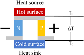
Figure 4. The model of one thermocouple in the TEG module.
Download figure:
Standard image High-resolution imageLet the Seebeck coefficient of the P-type and N-type semiconductor be  and
and  the output voltage of a single thermocouple will be:

where  is the absolute Seebeck coefficient between the two semiconductors, and its unit is V/K. Generally, the Seebeck coefficient S of a TEG module is given by:

where N is the number of semiconductor thermocouples in the TEG module, and  is the absolute Seebeck coefficient between the two semiconductors composing one thermocouple.
2.2.2. Peltier effect
Shown as figure 5, the Peltier effect describes when there is an electric current in a closed circuit composed of two different materials, the endothermic or exothermic phenomenon will occur at the connections of the two materials. Peltier effect is usually used for cooling or heating aims.

Figure 5. Schematic of Peltier effect.
Download figure:
Standard image High-resolution imageThe heat exchange value in Peltier effect is given by:

where π is the Peltier coefficient and I is the current in the loop. The unit of π is W/A.
2.2.3. Thomson effect
The Thomson effect describes the phenomenon that occurs when a current passes a conductor with a temperature gradient, the conductor will exchange heat with the surroundings through its surface. The amount of heat release or absorption is affected by the current direction and the conductor.
The amount of exchanged heat by the Thomson effect is given by:

where  is Thomson heat with a unit of W, β is the Thomson coefficient with a unit of V/K, I is the current passing through the conductor with a unit of A, and
  is the longitudinal position in the galvanic couple with a unit of m, so
  is a distribution function of the temperature in the galvanic couple.
2.2.4. Kelvin effect
The Kelvin effect summarizes the relationship between the Seebeck effect, Peltier effect, and Thomson effect. The relationship between the coefficients of these three effects is given by:


where  is the absolute Seebeck coefficient between the two materials (namely material a and b),
  is the Peltier coefficient between the two materials, T is the temperature, and
  and
and  are the Thomson coefficients of the two materials.
2.2.5. Joule effect
The Joule effect depicts that the conductor generates heat when the current passes through the conductor due to the resistance of the conductor. The heat produced by Joule effect is given by:

 is Joule heat, the unit is W; I is the current through the conductor, the unit is A; R is the conductor resistance, the unit is Ω.
2.2.6. Fourier effect
The Fourier effect is a simple thermal effect, which describes the relationship between the heat flowing through a conductor and the temperature at both ends of the conductor. Its expression is given as follows:

where  is the heat flowing through the conductor, the unit is W; λ is the thermal conductivity of the conductor, the unit is W/(m * K); L is the length of the conductor, the unit is m; a is the cross-sectional area of the conductor, the unit is m2.
2.3. Research progresses on TEG model
In addition to the above-mentioned effects, environmental factors will affect the characteristic of TEG modules. Therefore, it is difficult to derive the TEG output only from theoretical calculation. Recently, some researchers have obtained several approximate TEG models by ignoring some effects on the TEG module according to its working condition.
By ignoring the heat loss on the vertical direction of TEG current, paper [7] gives the internal temperature distribution function  of TEG and the relationship between absolute Seebeck coefficient α and temperature,

where

In equation (12),  and
and  are constants, L is the length of the semiconductor material,
  and
and  are the temperatures at TEG hot side and cold side, respectively.

where  is the reference absolute Seebeck coefficient and
  is a constant.
Then, the Seebeck coefficient of the whole semiconductor can be obtained:

By ignoring the Thomson effect and letting the temperatures on both sides of the TEG to be stable, paper [8] defines the Seebeck coefficient S as below:

where  is the maximum output voltage. For a given TEG module,
  is constants. Therefore, the paper [8] considers that the Seebeck coefficient S of a TEG are functions that are only affected by the temperature on hot sideof TEG, namely,

where a is constants.
Paper [9] proposes a new model of TEG and compares it with the results in [10]. The following functions are given in [9] by summarizing [10].


where  are constant.
It can be seen that Seebeck coefficient of a TEG is considered as quadratic functions to TEG's temperature and average temperature  is used to replace the temperature distribution function T (x) of the TEG.
Using the new model, paper [9] gives the following conclusions:

It is obtained by experimental testing on the TEG module proposed in [9].
It is clear that equation (19) given in paper [9] is the same to equation (15) presented in paper [8], and both can be written in the form of equation (16). In summary, although the authors in papers [7–10] try to generalize the relationship between the Seebeck coefficient of the TEG with its temperature distribution, their conclusions are not totally identical to each other.
3. Experimental setup and procedure
3.1. Experimental setup
To validate the proposed method, the experimental setup shown as figure 6 is used to conduct a series of experiments. The experimental setup consists of a heating furnace, a heat transfer box, two TEG modules with corresponding heat sinks, two thermocouples, two temperature measurement modules, and a laptop. The heat transfer box is a rectangular parallelepiped structure composed of stainless-steel plates to imitate the hot wall at industrial plants. Two TEG modules, TGM287–1.0–1.3 from European Thermodynamic [15], are pasted to the hot wall. However, only the copper heatsink on the top of the TEG modules can be seen in figure 5. The two TEG modules are independent of each other and can be used either alone or together in series or parallel connection. This research only uses the right TEG module. Two K-type thermocouples and two measurement devices (USB-TC01 from National Instruments Corporation), and a laptop are used to measure the hot and cold side temperatures of the TEG.

Figure 6. View of the experimental setup.
Download figure:
Standard image High-resolution image3.2. Experimental procedure
The first experiment is performed to determine the relationship between TEG open circuit voltage  and the temperatures at the TEG hot and cold side, namely
  and
and  The setting temperature of the heating furnace is 200°C. The hot wall temperature will increase from room temperature to its peak value and then decrease to room temperature after switching off the furnace. In this procedure,
 and
and  are measured by the multimeter and USB-TC01 and recorded by the laptop.
4. Experimental results
4.1.


The original data of 
 and
and  are shown as figure 7. The horizontal x-axis represents the sample time in this experiment, while the vertical axes are the temperatures at the TEG hot and cold side, and TEG open circuit voltage.

Figure 7. The recorded curve of 
 and
and 
Download figure:
Standard image High-resolution imageIn the heating procedure (form start point to point C), 
 and
and  gradually increases and reaches their maximum value at point C, while
  peaks at point A. The positions of maximal
  and
and  do not coincide because
  is not only influenced by
  but also by
  From point A to point B,
  decreases because the growth rate of
  is less than that of
  From point B to point C,
  maintains stable because the growth rate of
  is balanced with the growth rate of
The TEG module begins its natural cooling stage from point C, where the heating furnace is turned off. Both  and
and  gradually decreased in the cooling phase. There is a clear change in the temperature curve slope in the cooling stage because of the different sample intervals used in the data acquisition process.
Paper [16] explores the characteristic of a TEG exposed to a transient heat source on the hot side and natural convection on the cold side. The  curve depicted in figure 6 is similar to the results in [16], namely
  reaches its maximum value and then fells to a stable stage.
To explore the relationship between 
 and
and  the above experimental data are fitted in MATLAB. The results are given as follows:

where  is the coefficient of determination, the closer
  is to 1 means the higher fitting accuracy.
The comparison of the fitting result by using equation (20) and the measured value of  is shown as figure 8. It can be seen that the fitted result is very accurate.

Figure 8. Comparison of the fitting resultand measured value of TEG open-circuit voltage.
Download figure:
Standard image High-resolution imageAccording to figure 2, the TEG internal resistance  can be calculated by:

where, Voc can be calculated using equation (20) and Vout will be measured on-site.
From equation (20), the change of Seebeck coefficient S with the temperature difference  can be calculated by:

It can be seen that the forms of equation (22) is different from equations (14), (16), and (17). Such an accurate and linear relationship described in equation (22) has not been reported by other authors.
5. Results and discussion
5.1. The comparison of Seebeck coefficient
According to equations (15) and (19) proposed by paper [8] and [9],  is a constant. However, our research depicts the actual changing procedure of
  in figure 9. It can be seen that the value of
  varies with TH
and TC
.
varies with TH
and TC
.

Figure 9.
 changes with
  and
and 
Download figure:
Standard image High-resolution imageSince  and
and  in equation (12) cannot be obtained, the method proposed in [10] is adopted and the temperature distribution function T(x) is replaced by
  so that equation (14) can be written as:

Using the experimental data shown as figure 6 to equation (23), we can obtain that  = 50.71 and
  = 105.7.
Therefore, the model in [7] is approximately given by:

Using the experimental data shown as figure 6 to the equation (17) given in [10], we can obtain the value of  and rewritten equation (17) as:

The Seebeck coefficients calculated by equations (22), (24), and (25) are shown as figure 10. Comparing with the results obtained by using the methods in paper [7] and [10], the Seeback coefficient obtained by using the model proposed in this paper and equation (22) fits better with the experimental data.

Figure 10. The comparison of the Seebeck coefficient obtained by various models.
Download figure:
Standard image High-resolution image
6. Conclusion
To achieve the MPPT based-on internal resistance matching method for self-powered WSNs or IoT nodes using TEG, this paper proposes a simple approach to obtain the models of TEG's  the Seebeck coefficient and the internal resistance of TEG. The proposed method is verified by a series of experiments on a commercial TEG module: TGM-287–1.0–1.3 from Kryotherm. The experimental results indicate that the presented models are more accurate and simpler than the existing model reported by other authors.