
Abstract
This paper documents a new design for a vertical electrical impedance (VEI) scanner that has increased VEI scanning speeds by an order of magnitude. Specifically, a new impedance analyzer was designed with improved circuitry and signal processing; this analyzer is accurate over a large range of impedance magnitudes, has a high sampling rate, is inexpensive, has low power consumption, and has a small form factor. Additionally, the physical moving platform, the localization equipment, and the large-area electrodes (LAEs) of the VEI scanner were all significantly improved. The improved VEI scanner was used to scan a concrete bridge deck in a field demonstration. The VEI scanner was able to collect data at sufficiently high speeds to scan the bridge deck without stationary traffic control, and the resulting data were highly self-consistent and correlated well with both delamination and surface cracking data that were measured separately.
Export citation and abstract BibTeX RIS
Introduction
Bridges are critical elements of transportation infrastructure for which strategic preservation programs are warranted. In particular, if preventative maintenance can be applied early in the bridge deterioration process, the repair cost, which is estimated to be billions of dollars globally [1, 2], can be significantly reduced [3]. Because effective application of preventative maintenance requires accurate assessment of bridge condition, including assessment of non-visible defects, development of instruments for rapidly detecting defects and estimating their severity continues to be a prominent area of research [4–6].
Among the many elements of a bridge, the deck is one of the most difficult to inspect due to trafficking. Ideally, inspection techniques used to assess bridge decks would be both rapid and nondestructive to avoid the need for costly, disruptive, stationary traffic control and testing-related deck repairs. One recently developed inspection technique for concrete bridge decks involves measurement of vertical electrical impedance (VEI) [7–12]. Previous research has shown that VEI correlates well with other evaluation techniques such as chloride concentration and half-cell potential [8], which can be useful especially in preventative maintenance programs in cold regions and coastal regions in which concrete bridge decks are regularly exposed to salt.
While early versions of VEI measurement instruments were single-channel units that required the operator to drill a hole through the concrete to establish an electrical connection to the top mat of reinforcing bar, or rebar, the recent development of a multi-channel unit equipped with a large-area electrode (LAE) has enabled VEI measurements that are both rapid and completely nondestructive [7, 11]. This paper documents a new impedance analyzer that has further increased the scanning speed. Additionally, the physical moving platform, the localization equipment, and the LAEs have all been significantly improved. As a demonstration of the increased scanning speed of the new VEI apparatus, a concrete bridge deck was scanned without stationary traffic control, and the results were compared to delamination and surface cracking data that were measured separately.
Background
Electrical impedance is the alternating-current (AC) equivalent of electrical resistance and, for a homogeneous cylindrical material, can be written as

where  is the complex-valued electrical impedance,
  is the length of the cylinder,
  is the cross-sectional area, and σ is the complex-valued electrical conductivity of the material. The electrical conductivity of a material, σ, is proportional to the number of charge-carrying particles and their mobility within the material [13]. As equation (1) indicates, the measured impedance of a material is also influenced by the geometry of the material. Thus, while electrical conductivity may be intrinsic to a particular volume of concrete, for example, the measurement of impedance to infer electrical conductivity depends on the arrangement of the measurement probes in relation to the volume of material.
VEI measurements are acquired in the vertical direction, from the surface of the bridge deck to the top mat of rebar, as shown in figure 1. Because VEI is directly affected by the mobility of ions through the concrete matrix and any deck surface treatments or rebar coatings, VEI is a useful measurement of the protection provided to embedded rebar against chloride ingress through the surface of the bridge deck. Because chloride-induced rebar corrosion is a primary deterioration mechanism in concrete bridge decks [4, 6], quantifying the protection against chloride ingress, or the ingress of other deleterious agents, is a key aspect of determining current bridge deck condition and estimating future deterioration rates.
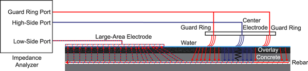
Figure 1. Cross section of a bridge deck and guarded VEI measurement to quantify the cover protection provided to the rebar, with blue and red lines representing the currents that flow through the center electrode and the guard ring, respectively.
Download figure:
Standard image High-resolution imageThe electrical impedance of an interrogated material system is most often measured using the complex version of Ohm's law:

where  is the complex-valued impedance,
  is the complex-valued voltage potential difference across the system, and
  is the resulting complex-valued current. These three variables are functions of the measurement frequency,
  and are often reported as a magnitude and phase. Previous research has shown that the magnitude of
  at frequencies between 100 Hz and 1 kHz correlates well with important bridge deck performance parameters [14–16].
The geometry, placement, and electrical connection of probes needed to perform VEI measurements are important [7, 11, 17]. To couple the probes electrically to the bridge deck, a coupling fluid, usually water, is placed on the surface [7–11, 14]. The high-side port of an impedance analyzer, which provides the voltage source and facilitates the current measurement, is connected to a probe on the surface of the bridge deck. The low-side port, which is the effective electrical ground, is connected to an LAE(s) that provides a low-impedance connection to the underlying rebar [7]. The deck area interrogated by a VEI probe is controlled by placing a guard ring around the probe, or center electrode, to electrically isolate it [18]. By measuring the current through only the center electrode, the impedance measurement is effectively constrained to the material directly under the probe, as depicted in figure 1 [7, 19].
A guard ring applies the same voltage to the surface in contact with the guard ring as the surface in contact with the center electrode, reducing horizontal current flowing from the center probe [7] and thereby improving the accuracy of the impedance measurement by consistently constraining the measurement area [19, 20]. The electrical currents from both the guard ring and the center electrode combine additively at the low-side port as shown in figure 1. Measurement of the combined currents through the low-side port would result in non-spatially-confined and non-isolated impedance measurements, while measurement of the current flowing through only the center probe results in a spatially-confined and isolated impedance measurement.
For the VEI scanner, a commercially available impedance analyzer was desired. However, most commercially available impedance analyzers measure the current at the low-side port through a transimpedance measurement configuration. To support a guard ring and a high measurement rate, a custom impedance analyzer was necessarily designed for these measurements. Additional design specifications for the impedance analyzer developed from previous research and bridge testing were as follows [8, 11, 12, 14]:
- Network capable
- Reconfigurable measurement frequency: 100 Hz to 1 kHz
- Low impedance measurement: 1 kΩ
- High impedance measurement: 1 MΩ
- Measurement accuracy: <10% absolute error
- Measurement rate: >50 samples/second
- Power consumption: <5 W
- Size: <0.2 m3
- Mass: <10 kg
The objective of this work was to design, construct, and deploy an impedance analyzer that met these specifications for VEI scanning of a bridge deck in the field.
Impedance analyzer
To meet the desired specifications, the impedance analyzer was designed as a mixture of analog and digital subsystems. The analog subsystem consisted of circuitry designed to generate a high-quality sinusoid signal and measure the resulting  and
and  signals expressed in equation (2). The digital subsystem consisted of signal-processing schemes designed to remove noise from the
  and
and  signals and compute
  The analyzer platform was a FRDM K64F (NXP) development board with a 120-MHz microcontroller with direct memory access (DMA) and an integrated 12-bit digital-to-analog converter (DAC) and two 16-bit analog-to-digital converters (ADC) [21].
Analog and digital subsystems
Analog design
The analog subsystem is shown in figure 2. The voltage signal output of the DAC is a 3.3-Vpeak-to-peak sinusoid at the desired measurement frequency, typically 100 Hz to 1 kHz. This sinusoid signal is precomputed on the microcontroller, and the voltage output is updated at 100 kHz using DMA. The stair-step output is smoothed by a second-order Sallen-Key reconstruction filter with a corner frequency of 3.1 kHz. The signal passes through a second-order Sallen-Key high-pass filter with a corner frequency of 19.4 Hz to remove the DC offset resulting from the DAC.

Figure 2. Analog circuitry of the high-side impedance analyzer with guard ring capability showing the analog filters and measurement circuitry.
Download figure:
Standard image High-resolution imageAfter passing through the analog filters, the signal passes through a 51-kΩ current-sense resistor. A resistance of 51 kΩ was chosen because it balances the signal-to-noise ratio (SNR) for both the voltage and current signals over a large range of expected concrete impedance values, which are typically 1 kΩ to 1 MΩ. When the resistance is 1 kΩ, the  signal is approximately 0.064 Vpeak-to-peak, and
  is approximately 3.24 Vpeak-to-peak. When the resistance is 1 MΩ, the
  signal is approximately 3.14 Vpeak-to-peak, and
  is approximately 0.16 Vpeak-to-peak. The current flow through the current-sense resistor is converted to a voltage signal using an instrumentation amplifier (INA121P, Texas Instruments) with a gain of 1. A 1.65-V DC bias is added to the instrumentation amplifier in order to center the signal between the 0-V and 3.3-V rails of the ADC.
After the signal passes through the 51-kΩ current-sense resistor, another instrumentation amplifier (INA121P, Texas Instruments) is used to measure the voltage difference between the impedance probe and the low-side port, again applying a 1.65-V offset to the output before sampling with a separate ADC. An additional amplifier in a voltage-follower configuration passes the signal from the probe to the guard ring.
Digital design
In the digital subsystem, the voltage and current signals are synchronously sampled at 100 kHz. Sampling is triggered by a programmable delay block (PDB), and values are stored in a double buffer using DMA. While one buffer is filled with samples, the other buffer is processed by the filtering scheme shown in figure 3. Each box represents a decimating low-pass filter, with the decimation factor labeled in the middle of the box. Information about the passband, stopband, and attenuation of each filter is also given in figure 3. The low-pass filters are necessary to reduce the effects of noise, aliasing, and other channel interference. The sine and cosine in the filtering schematic demodulate the signal at the center frequency [22]. Magnitude and phase are then estimated using in-phase and quadrature components of the signal that have been further processed.

Figure 3. Digital signal-processing scheme for the impedance analyzer.
Download figure:
Standard image High-resolution imageThis overall signal-processing scheme is applied to both the voltage and current signals so that the complex impedance can be calculated using equation (2). An impedance measurement with an effective bandwidth of 40 Hz is recorded 98 times per second. This data collection rate is more than an order-of-magnitude improvement over that of previous VEI scanning devices, which employed a resistor-switching configuration and only generated measurements approximately four times per second [8].
Laboratory evaluation
The analog and digital subsystems resulted in the impedance analyzer shown in figure 4. The impedance analyzer consumes only 1.2 W of power (5 V at about 240 mA of current draw). The impedance analyzer weighs 72 g and is very small, having dimensions of 9 cm by 6 cm by 4 cm.

Figure 4. Impedance analyzer with power and data transfer connections through the USB cable and center electrode and guard ring connections through the coaxial cable.
Download figure:
Standard image High-resolution imageA decade resistor (1434-G, General Radio) with a range from 0.1 Ω to 1 MΩ was used to evaluate the accuracy of the newly developed impedance analyzer. Figure 5 shows the measured voltage and current signals for resistances of 1 kΩ and 1 MΩ at a measurement frequency of approximately 190 Hz. Figure 5 also shows an estimate of the power spectral density of the signal using Welch's method to estimate the power spectrum. The recorded signals were within the desired peak-to-peak voltages for proper ADC measurements, the signal-to-noise ratio was at least 30 dB in the worst case, and the largest harmonic peak (at an integer multiple of 190 Hz) was more than 20 dB below the primary peak (at 190 Hz) in the worst case.
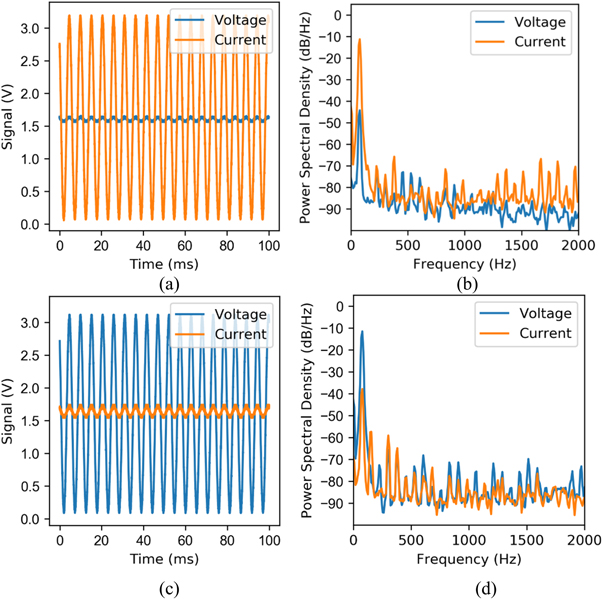
Figure 5. (a) Voltage and current signals at a generated frequency of approximately 190 Hz recorded by the impedance analyzer with a 1-kΩ load. (b) Estimated power spectral density of the voltage and current signals of part (a) using Welch's method. (c) Voltage and current signals at a generated frequency of approximately 190 Hz recorded by the impedance analyzer with a 1-MΩ load. (d) Estimated power spectral density of the voltage and current signals of part (c) using Welch's method.
Download figure:
Standard image High-resolution imageAn additional three sets of measurements were also obtained. First, resistor values between 0 and 10 kΩ were measured in step sizes of 100 Ω. Second, resistor values ranging from 0 to 100 kΩ were measured in step sizes of 1 kΩ. Third, resistor values ranging from 0 to 1 MΩ were recorded in step sizes of 10 kΩ. Each resistor value was measured for approximately 1 s by the impedance analyzer. The mean and standard deviation of the impedance magnitude for that second were recorded. The scanning frequency for this test was 568 Hz, which was selected because it was approximately in the middle of the scanning frequency range of interest.
The results of this experiment are shown in figure 6. Figure 6(a) shows the measured resistance compared to the actual resistance, with an ideal measurement being represented by the line of equality displayed in the plot area. Figure 6(b) shows the percent error of the measured resistance as compared to the actual resistance. The first seven points equally spaced between 100 Ω and 700 Ω have errors as high as 60% but are not shown since they are outside the designated measurement range. Figure 6(c) shows the estimated standard deviation of the measurement noise using approximately 100 samples collected for each data point. Figure 6(d) shows the standard deviation as a percentage of the actual resistance value. The horizontal axes of each subplot and the vertical axes of 6(a) and 6(b) are presented on a logarithmic scale where a value of 2 represents 100 ohms, a value 3 represents 1 kΩ, and so on.
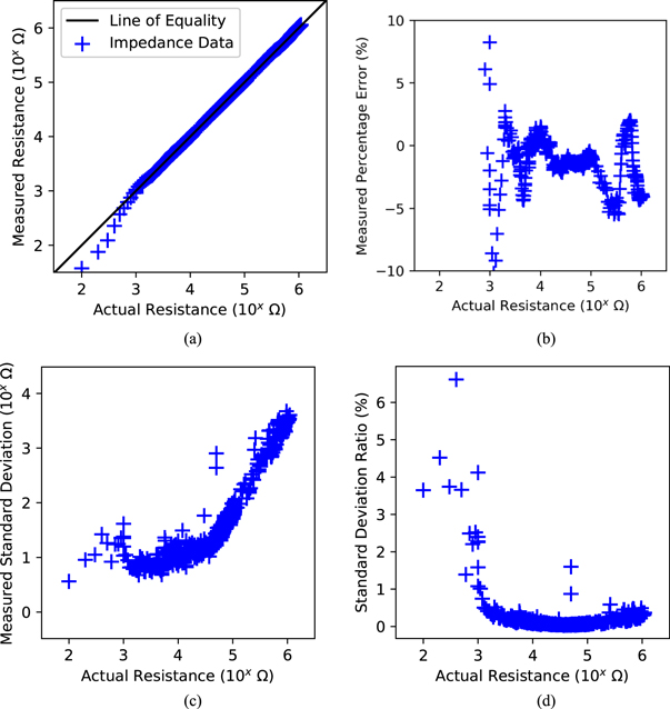
Figure 6. (a) Measured magnitude versus actual magnitude. (b) Percent error of measured magnitude versus actual magnitude. (c) Estimated standard deviation of each measurement point. (d) Standard deviation shown as a percentage of the actual impedance value.
Download figure:
Standard image High-resolution imageFigures 6(a) and (b) demonstrate that the impedance analyzer accurately estimated actual impedance in the range of 1 kΩ to 1 MΩ, which is the full range indicated in the desired specifications. The accuracy was consistently within 10 percentage points in the impedance range of interest and was usually accurate to within 5 percentage points. Below the low impedance measurement limit of 1 kΩ, the impedance measurements develop a distinct bias due to a non-zero voltage bias in the voltage signal assumed to be caused by noise and possible leakage currents. This bias is insignificant when the voltage signal is large but becomes significant at smaller resistances when the signal is small. Although outside the range of the decade resistor and above the high impedance measurement limit, a similar effect, not shown in this data, happens to the current measurement when impedance values larger than 5 MΩ are measured. Despite bias when measuring relatively low and high impedance values, the impedance analyzer has low variance. As shown in figure 6(d), the standard deviation of the error is often less than 1% of the actual value.
These evaluations demonstrate that the new impedance analyzer meets the desired specifications and is capable of measuring the impedance of a bridge deck to within 10% of the actual impedance within the designed measurement range and at high sample rates. The new design can also drive guard rings and be arranged in a multi-channel configuration. These features should allow the impedance analyzer to be successfully deployed in field studies to measure the protection provided to embedded rebar against chloride ingress through the surface of bridge decks.
Multi-channel VEI bridge deck scanner
Scanner design
A multi-channel VEI scanner was constructed using one impedance analyzer per channel. This scanner, shown in figure 7, consisted of a data collection unit, a multi-channel impedance analyzer, a water delivery system, a localization unit, a moving platform, LAEs, and probes.
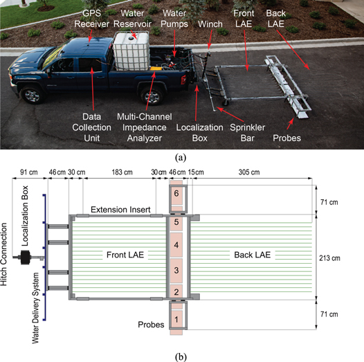
Figure 7. (a) Photo of the VEI scanner mounted to a truck. (b) Schematic of the moving platform portion of the VEI scanner.
Download figure:
Standard image High-resolution imageA pickup truck was used to tow the scanner, as shown in figure 7(a). The data collection unit, pictured in figure 8, was housed in the cab of the truck. The data collection unit was comprised of five time-synchronized, single-board computers that recorded multiple data types; the parallel configuration of the single-board computers allowed for recording of multiple data streams with large bandwidth.

Figure 8. Data collection unit.
Download figure:
Standard image High-resolution imageA waterproof box in the truck bed housed six impedance analyzers as shown in figure 9. Each impedance analyzer shared a common low-side port connection and was connected to a single USB hub. The hub was connected to the data collection unit via a 5-m USB 3.0 extension cable. Six 7.6-m BNC cables connected the center electrode and guard ring of the probes to the high-side and guard ring ports of the impedance analyzers. The low-side ports were connected with wires to the aluminum frame of the moving platform, which was electrically connected to the LAEs.
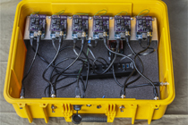
Figure 9. Multi-channel impedance analyzer.
Download figure:
Standard image High-resolution imageA 1000-L water reservoir located in the truck bed was the source of water for the water delivery system. The water reservoir was connected to three pumps, each capable of supplying 20 l per minute, that were powered by a 12-V battery. The pumps supplied water to a sprinkler bar through three standard garden hoses, as depicted in figure 10. Multiple sprinklers were mounted to the bar to ensure sufficient application of water to the deck surface during scanning [10].
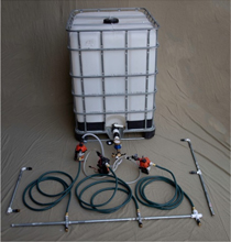
Figure 10. Water delivery system with the sprinkler bar separated into three pieces.
Download figure:
Standard image High-resolution imageA hitch extension with a localization unit was attached between the truck hitch and the moving platform [23]. The box contained two sideways-pointing light detection and ranging (LIDAR) units and a downward-facing camera, as shown in figure 11. A differential global positioning system (GPS) unit was also used for localization. The GPS receiver was located in the truck cab, and the GPS antenna was placed on top of the cab. The LIDAR units were used to determine the distance of the scanner from the parapet walls for estimating transverse position. The camera was used to identify the exact time the scanner crossed onto the bridge, and the GPS was used to estimate longitudinal position within 1 m [24].

Figure 11. Localization box containing synchronization electronics, two LIDAR units, a downward-facing camera, and a laser ruler.
Download figure:
Standard image High-resolution imageThe hitch extension was connected to the aluminum frame of the moving platform using a solid steel hitch bar and a double-hinged bracket. A steel post extended 1.2 m upwards from the hitch bar, and an 1130-kg winch (Badland) was attached to the top of the post. The winch was used to lift the platform off the ground for easy relocation during scanning or to fully stow the platform for travel between bridges, as shown in figure 12.
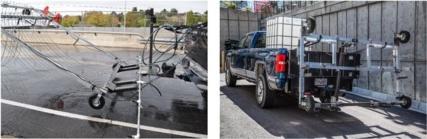
Figure 12. (Left) Moving platform being lifted off the ground by the winch. (Right) Moving platform in a stowed configuration.
Download figure:
Standard image High-resolution imageThe LAEs and probes were attached to the moving platform as shown in figure 7. The front LAE was positioned in the open frame area in front of the line of probes, and the back LAE was positioned directly behind the line of probes. These LAEs created a continuous low-impedance connection to the rebar, even when the scanner was traversing joints between electrically discontinuous spans in a bridge deck [7, 11]. The six probes between the LAEs were attached using flexible connections to the aluminum frame. Two of the probes were attached to optional wings that extended the 2.4-m scanning width to 3.7 m. Each probe used a different measurement frequency to mitigate probe crosstalk. The frequencies used were 190, 272, 347, 431, 500, and 568 Hz. The LAEs, probes, and extension bars were removed when traveling between scanning sites as shown in figure 12(b).
The probes and LAEs were designed to be mechanically robust and also flexible to ensure consistent contact with the bridge deck during scanning. Guarded probes were made of flexible brushes. As shown in figure 13, the center electrode and guard ring of a probe consisted of numerous 26-cm strands of 0.8-mm-diameter 302/304 stainless steel cables folded in half and individually threaded through two separate holes in perforated metal strips. Four of these metal brush strips were arranged into a diamond shape to form the guard ring brush and attached to a plastic frame having dimensions of 0.6 m by 0.5 m by 0.02 m. The center electrode consisted of a separate metal brush strip attached to the center of the plastic frame. This flexible brush design allowed the probe to conform to the contours of the bridge deck surface and maintain a relatively consistent contact area while exhibiting excellent durability even on very abrasive deck surfaces. The diamond shape for the guard ring was preferred over a rectangular shape as it resulted in more uniform bending of the individual metal bristles.
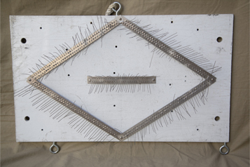
Figure 13. Guarded probe with center electrode made of stainless steel bristles.
Download figure:
Standard image High-resolution imageThe LAEs were designed to slide easily over the bridge surface. The LAEs were sets of 7-mm-diameter galvanized steel cables connected in parallel to 2-m aluminum bars. The bars electrically connected the cables to the frame. The weight and flexibility of the cables allowed the LAEs to conform to uneven surfaces. These cables were oriented in the direction of travel to minimize snagging and collection of debris, which were both significant problems with previous designs. The cables did not exhibit noticeable wear after multiple passes across bridge decks.
Field evaluation
For a field evaluation, the VEI scanner was used to scan a concrete bridge deck in northern Utah. This bridge deck, pictured in figure 14, was built in 1995. It has a two-span cast-in-place concrete deck with a bare concrete surface and is supported by continuous steel girders. The bridge deck is 78 m long and 13.6 m wide (as measured from the outsides of the parapet walls) and carries two lanes of traffic on an urban local road with an estimated average daily traffic (ADT) of 5000. The bridge deck is typically subjected to numerous deicing salt applications as part of winter maintenance each year.
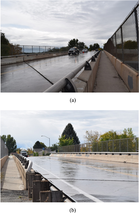
Figure 14. (a) Photograph of VEI bridge scanning. (b) Photograph of the entire bridge during testing.
Download figure:
Standard image High-resolution imageThe field evaluation consisted of five bridge deck scans using the VEI scanner, where a scan included one pass in each lane of the bridge deck. Each pass scanned a width of 3.7 m and was performed at a speed of 5 to 7 km h−1, which required approximately 150 s to complete. During each pass, a sufficient quantity of plain tap water was sprayed onto the deck surface to produce a thin film of water as shown in figure 14(b). The data were recorded using the data collection unit and were processed afterwards by reconstructing the scanning paths and associating impedance measurements with their respective locations.
This bridge deck was of particular interest for the field evaluation because delamination and cracking surveys had already been performed on this deck approximately 8 months prior to the VEI scanning. The high-resolution delamination map was generated through a detailed chain-drag survey that required about 60 man-hours, not including personnel who were responsible for traffic control. Crack mapping was completed more rapidly, with only those cracks that were clearly visible from a standing position, or about 1.5 m from the deck surface, being recorded. Crack mapping required about 2 man-hours to complete. Both the delamination map and crack map were digitized after the surveys were completed.
The maps produced in this study are shown in figure 15. Figures 15(a) to (e) are the VEI maps from the five bridge deck scans, while figure 15(f) shows the delaminations and cracks together on the same plot. VEI is displayed on a logarithmic scale, similar to the values shown in figure 6. In preparation of the maps, linear interpolation was used to compute values for areas between measurement points. (Linear interpolation was also used to replace invalid data collected by one probe that was determined after the scanning to have a faulty connection.).
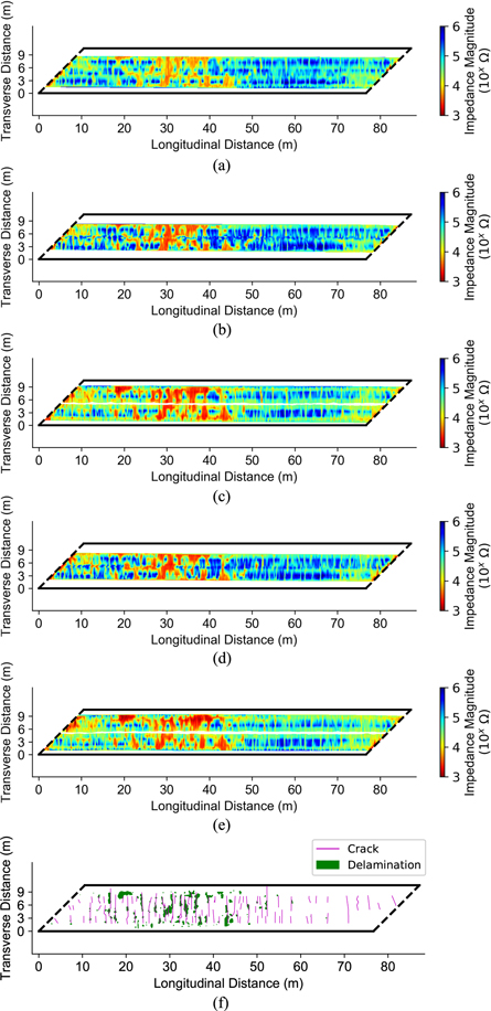
Figure 15. (a)–(e) VEI results for all five scanning passes. (f) Results of chain-drag survey (green) and crack mapping (magenta).
Download figure:
Standard image High-resolution imageA visual comparison of the VEI maps with each other indicates a high level of consistency among the five passes. Pass 1 appears to have slightly higher VEI values than the subsequent passes, which was expected as the water applied to the deck was still soaking into the concrete; for this reason, pre-wetting the deck or applying multiple passes is recommended to obtain stable readings. Passes 2 to 5 have very similar results, with most discrepancies being attributable to minor spatial offsets and interpolation.
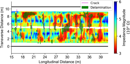
A visual comparison of the VEI maps with the delamination and crack maps, as illustrated in figure 16 for a portion of the deck, also indicates strong correlations. Specifically, almost all of the detected delaminations occur in areas with very low VEI values (<5 kΩ), and the very low VEI values beyond the edges of many delaminations suggest the locations of future delamination growth. Similarly, nearly every crack that was recorded in the cracking survey occurs in an area with low VEI values (5 kΩ to 50 kΩ). Additional linear features also characterized by low VEI values, but not corresponding to a recorded crack, may indicate cracks that formed between the cracking survey and the VEI scans, or they may indicate future crack locations. Because VEI values can be used to quantify the spatial extent and severity of compromised concrete, VEI maps may be more useful than delamination or cracking maps for delineating areas of a concrete bridge deck that warrant repair.
Figure 16. Comparison of VEI maps with delamination and crack maps for a portion of the bridge deck.
Download figure:
Standard image High-resolution image
Regarding the speed of data collection, the VEI scanning was completed at a rate comparable to that of visual inspection and more than 500 times faster than the chain-drag survey. Regarding data analysis, post-processing of the collected VEI data was automated and required less than an hour to complete. Given that the speed of VEI scanning is approximately the same as that of a street sweeper, nominally 5 to 10 km h−1 [25], VEI scanning could likely be performed on non-highway bridges with minimal traffic control.
Conclusion
A complete multi-channel VEI bridge deck scanner capable of scanning bridges at high speeds was developed in this study. For use in the scanner, a new network-capable and configurable impedance analyzer with guard ring support was designed. This analyzer is accurate to within 10% for impedance values ranging from 1 kΩ to 1 MΩ, has a measurement rate of 98 samples per second, consumes less than 2 W of power, and has a small form factor; for these reasons, the impedance analyzer may also be useful in a variety of other applications, especially those for which high-side impedance measurements are needed. The multi-channel VEI scanner was able to collect data at sufficiently high speeds to scan a bridge deck without stationary traffic control, and the resulting data were highly self-consistent and correlated well with both delamination and surface cracking data that were measured separately.
In summary, the new VEI scanner can be highly beneficial to engineers and contractors involved in concrete bridge deck management. It allows early detection of non-visible defects while minimizing the need for stationary traffic control during testing. Future research will examine the performance of the VEI scanner on bridge deck overlays and investigate the relationship between VEI measurements and other standard bridge deck condition assessment techniques.
Acknowledgments
The authors acknowledge support for this project from the National Cooperative Highway Research Program IDEA program and the Nebraska Department of Roads. The authors also thank research assistants in the BYU Materials and Pavements Research Group for their assistance with the chain-dragging and crack-measurement surveys.