

Abstract
The miniature heater assembly has been developed for a compact portable battery powered thermo-luminescence (TL) reader system. The construction and thermodynamics of this heater assembly has been described in detailed. The theoretical modeling of the heating processes participating in the heater assembly has been evolved and substantiated with experimental evidential analysis. The heat generation rate equations have been formulated by considering the radiative and conduction losses. The formulated theoretical model matches well within the experimental findings under some assumptions made in generation of linear/non-linear and constant temperature heating profiles for a variable heating rate in the range of 0.1 K s−1 to 4 K s−1 with maximum temperature of 400 °C. The developed miniature heater assembly was installed in newly designed battery powered TL reader system. This TL reader system works on four 1.2V, 2.8Ah, Ni-Mh re-chargeable batteries. The TL glow curve of α-Al2O3:C, CaSO4:Dy, and LiCaAlF6:Eu,Y (LCAF) phosphor were recorded using the developed heating assembly.
Export citation and abstract BibTeX RIS
1. Introduction
Many decades of extensive research and development has made the phenomena of thermo-luminescence (TL) and optically stimulated luminescence (OSL) valuable investigating tool in various field of applications, like environment/personnel monitoring, geological/archeological dating, medical dosimetry, space dosimetry and more recently in nuclear forensic [1–5]. However, both these techniques are having their own advantages and disadvantage in terms of their use and methods of getting luminescence signals [6]. In OSL method, the optical stimulation results in release of the trapped charges from meta-stable defects and there subsequent recombination with charges of opposite polarities lead to luminescence signal. Thus, the OSL dosimetry offers advantage in terms of sensitivity, relative easy, fast and multiple readout choice. However, the OSL dosimeters should be handled in dark condition during exposure storage and readouts. This condition may impose some limitation for use the OSL dosimeters in field conditions under nuclear/radiological emergencies. These constrain gives added advantage for the possibility of developing a portable OSL reader operating at low electrical power ∼2 Watt [7]. On the other side, most of the TL phosphors can be irradiated and handled in an ambience light. However, TL glow curve recording requires heating of a reasonable amount of the phosphors, hence needs a substantial thermal/electrical power. In most of the available commercial TL reader system consumes ∼120 Watt (AC mains (220V@50Hz)) electrical power to achieve desirable heating rate (0.1 K s−1–20 K s−1) and attending maximum temperature of ∼450 °C. Thus, the development of compact, portable, high sensitive battery powered TL reader would be of great utility for infield radiological radiation measurements applications using TL dosimetry. This kind of TL reader also provides an alternate low cost effective system for a laboratory of the universities involved in TL research activities. The development of such battery powered TL reader system required construction of an efficient miniature heater assembly. The present paper describes the design and associated development aspects of a miniature TL heater assembly. This is further installed in programmable low cost compact 'Battery Operated TL Reader' (BOTLR-1) system. This TL reader system has been designed to record TL glow curves by heating <50 mg of TL phosphor linearly up to 400 °C. The BOTLR-1 system operates on 5V, DC at ∼13 Watt electrical power using four rechargeable Ni-MH, 4 AA (1.2 V) batteries. The reader provides great dynamic heating rate range from 0.1 K s−1 to 4 K s−1. The typical TL glow curves have also been recorded for CaSO4:Dy and commercially available α-Al2O3:C phosphors on this reader system.
2. Materials and methods
2.1. Experimental setup
The miniature TL heating assembly consists of the nichrome wire (0.14 mm, 38 AWG, 2Ω) as a heating element which is fixed below an electrically isolated kanthal planchet strip (20 mm × 12 mm × 0.25 mm) and having electrical insulation of mica shown in figure 1. To prevent the radiative and convection loses a lower section of the heating element is covered with heat insulation materials. The K- type thermocouple wire (0.1 mm dia.) is welded at kanthal planchet as shown in figure 1. The Phillips P89C51RD2 microcontroller based embedded system provides the control of complete hardware process. The desirable voltage profiles have been generated using 12- bit serial ADC, MAX1214 with appropriate active low pass filter. The current to the nichrome heater element is being measured by 12 bit ADC MAX 539 coupled with required Op-Amp instrumentation amplifier. The proportional, integral and differential (PID) based heater current control circuit is employed for controlling the temperature of this miniature TL heating assembly. All other exposed sides of the kanthal strip were covered with heat insulation material to minimize the heat loss to the surrounding environment. The TL detection module is consists of an EMI 9125B, PMT (utilizing BG-39 optical filter across photocathode) with user defined variable PMT bias voltage and current to frequency (I/F) convertor.
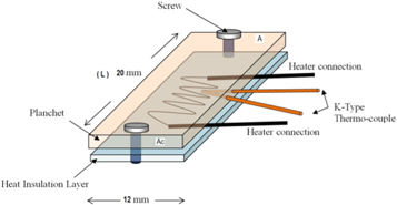
Figure 1. Construction diagram of the miniature heater assembly of BOTLR-1 system.
Download figure:
Standard image High-resolution imageThe developed miniature TL heating assembly for BOTLR-1 system is depicted in figures 2(a) and (b). This TL reader system operates on four 1.2 V, AA size, Ni-MH reachable batteries. Once fully charged provides twenty TL readouts with a linear heating rate 3 K s−1 up to maximum temperature of 400 ºC.

Figure 2. (a) The BOTLR-1 systems. (b). BOTLR-1 system with a loaded sample TL dosimeter.
Download figure:
Standard image High-resolution image2.2. Theory
2.2.1. Basic theory of resistive joule heating
The resistive heating element having resistance of RH (Ohm) generates a heat dH(t) (Calories) under current IH (t) (Ampere) passing through it for time dt (s) can be derived in term of potential difference V(t) (Volt) developed across resistive element as


Where, 'J' is mechanical equivalent of heat (J = 4.184 J cal−1)
The associated potential difference can be expressed as

Incorporating equation (3) in (2), we get


This relationship is known as Joule's first law or Joule–Lenz law [8, 9]. The most of the TL readouts have being carried out with various temperature profiles, apart from generally utilized iso-thermal (constant temperature) and linear heating [10, 11]. The desirable temperature verses time profiles have been achieved by feeding programmable analog voltage V (t) to the temperature control circuits. The most generalized form of voltage verses time profile used in such circuits are described as [12, 13]

Where, k is constant having dimension of Volt s−l, and l the dimensionless number termed as 'Time Base Power' (TBP), can have values 0 ≤ l ≤ ∞ [14]. This voltage profile will lead to a modulation of the heater DC current with use of MOSFET/transistor and under AC current supply, phase angle control by SCR (Silicon Control Rectifier) is used for this purpose. Therefore, for present heater element this DC current modulation can be expressed as

Where, ξ is proportionality constant with unit 'A/V' and takes constant value for most of designed heater circuit. In practice, the heating is carried out either by the linear increasing or constant temperature profiles with respect to time. These two cases can be expressed by assuming l = 1 or l = 0 in above equation (6b), respectively. Further the heating profiles can be given as
Linear

and constant heating linear

Where, ko: takes constant value with unit (V).
2.2.2. Analysis under adiabatic complete thermally isolated system
Here, we assumed that the resistive heating element is fully covered with heat insulation material, thus does not have any privilege of exchanging a thermal energy with the surrounding environment. Under above assumption equation (5), presents the amount of heat generated in resistive heating element due to current IH(t) passing through it. This results in an increase of temperature dT. Now the amount of heat energy associated with the heating element can be expressed as

Here, C is specific heat capacity of solid expressed in [kJ/kg/K] cal/g-K and 'm' is the mass of heating element expressed in gram [1 kJ kg−1 = 0.2390 kcal kg−1]. In present assuming all the heat energy generated in heating element contributes for increase in temperature. We can incorporate equation (6c) in equation (5) and equating to equation (7) as

When 'C' is in SI unit the above equation can be further expressed as

Integrating equation (8b) from initial start temperature To to the final temperature T in time 't ' for maximum allowed current Imax, we get

Here,


From equation (8a)


Here,  is the electrical power (Watt) delivered to the resistive element. Further, re-arranging the terms in equation (9a), we get,

Let's define  is Effective Heating (EH) rate expressed in K s−1. Under this assumption equation (9b) becomes

Here, the value of β(t) increases with increase in the power delivery to the resistive element and decreases with both, increase in mass as well as heat capacity of the heating element along with TBP (l). For the condition of constant current (Io) passing though resistive element with respect to time, i.e. l = 0; the equation (6d), reduces to

Equating equations (9c) and (10a), we get constant heating rate and heating profile as


The equation (10c) gives the linear profile of temperature with constant heating rate  for given constant heater element current. The whole heater assembly is composite in nature and consists of different materials, having different heat capacities as shown in figure 1. Thus, it is more practical to consider the combined effect of all the different components contained inside the heater system. Therefore, lets re-define the EH rate as

Where, (Cm)H is the effective combined heat capacity - mass product which is a weighted average for all the different heater components including TL phosphor material. In practice for such miniature heater a TL phosphor of considerable large mass will affects the performance of heating system. However, the temperature feedback mechanism will defiantly negate this effect up to a greater extent. Further simplifying the equation (10d) as

Where, ![$\psi =\left[\tfrac{{{\rm{R}}}_{{\rm{H}}}}{{({\rm{C}}{\rm{m}})}_{{\rm{H}}}}\right]$](https://content.cld.iop.org/journals/2631-8695/2/2/025032/revision2/erxab9026ieqn4.gif) is a new parameter termed as 'Heating Rate to Current Coefficient' (HRCC) expressed in K/(s.A2). The HRCC can be measured experimentally by applying a constant current to the heating element under feedback mechanism deactivated. The figure 3 shows the temperature profiles with respect to time of designed TL heater strip under various constant heater currents IH for above discussed condition. The data corresponding to the initial ∼5% of the temperature profiles (as shown in figure 3) is considerably good approximation for fitting equation (10d). This assumption is being supported by the fact that at a higher temperature the heat associated with heating assembly increases and leads to deviation of the temperature profile from equation (10d). The EH rate βo for different constant heater current can be determined from linear fit to initial temperature profiles discussed above. The determination of slope of the line fitted to experimental data (figure 4) of heating rate 'β' versus heater current I2H, gives the HRCC parameter value ∼8.39 (K/s.A2) with intercept at β – axis of ∼0.47. This offset of EH rate (βo) is due to the variation in ambience temperature of the heater assembly. Considering the measured value of HRCC for 2 Ω resistance of the nichrome wire the value of (Cm)H for this kanthal planchet can be estimated from the definition of ψ introduced in equation (10e) as 0.23 J K−1. For present kanthal strip planchet (shown in figure 1, dimension 2.0 × 1.2 × 0.025 cm , density 7.1 g/cc) with assuming specific heat capacity(C) at 200°C as 0.56 J g−1 K−1, the calculated value of (Cm)H turned out to be ∼0.22 J K−1. In this analysis we have ignored the contribution to composite heat capacity from nichrome wire due to its negligible mass with compare to the kanthal planchet. However, the close agreement between measured and estimated values of (Cm)H shows imperceptible effect of a composite structure on the heat capacity as compared to kanthal planchet. Therefore, the basic thermal load other than kanthal planchet can be ignored in further discussion. Let us consider a more generalized form of the heating profiles for different TBP (l) values as expressed in equation (8e)
is a new parameter termed as 'Heating Rate to Current Coefficient' (HRCC) expressed in K/(s.A2). The HRCC can be measured experimentally by applying a constant current to the heating element under feedback mechanism deactivated. The figure 3 shows the temperature profiles with respect to time of designed TL heater strip under various constant heater currents IH for above discussed condition. The data corresponding to the initial ∼5% of the temperature profiles (as shown in figure 3) is considerably good approximation for fitting equation (10d). This assumption is being supported by the fact that at a higher temperature the heat associated with heating assembly increases and leads to deviation of the temperature profile from equation (10d). The EH rate βo for different constant heater current can be determined from linear fit to initial temperature profiles discussed above. The determination of slope of the line fitted to experimental data (figure 4) of heating rate 'β' versus heater current I2H, gives the HRCC parameter value ∼8.39 (K/s.A2) with intercept at β – axis of ∼0.47. This offset of EH rate (βo) is due to the variation in ambience temperature of the heater assembly. Considering the measured value of HRCC for 2 Ω resistance of the nichrome wire the value of (Cm)H for this kanthal planchet can be estimated from the definition of ψ introduced in equation (10e) as 0.23 J K−1. For present kanthal strip planchet (shown in figure 1, dimension 2.0 × 1.2 × 0.025 cm , density 7.1 g/cc) with assuming specific heat capacity(C) at 200°C as 0.56 J g−1 K−1, the calculated value of (Cm)H turned out to be ∼0.22 J K−1. In this analysis we have ignored the contribution to composite heat capacity from nichrome wire due to its negligible mass with compare to the kanthal planchet. However, the close agreement between measured and estimated values of (Cm)H shows imperceptible effect of a composite structure on the heat capacity as compared to kanthal planchet. Therefore, the basic thermal load other than kanthal planchet can be ignored in further discussion. Let us consider a more generalized form of the heating profiles for different TBP (l) values as expressed in equation (8e)
Now introduce a new parameter 'ω' as a parameter having dimension of K/s2l+1

Thus equation (8e) become

For a linear increase in heater current IH(t) with respect to time i.e. TBP (l) = 1, we get


Figure 3. Generated temperature profiles under no feedback condition for the constant step heater currents (IH), (A) IH = 1.4 A, (B) IH = 0.8 A, and (B) IH = 0.3 A.
Download figure:
Standard image High-resolution image
Figure 4. Variation of heating rate β with respect to square of the different open loop (no feedback) constant heater current I2H(A2).
Download figure:
Standard image High-resolution imageTherefore, the linear increase in heater current with respect to time results in non-linear increase in temperature as depicted from equation (11c). The numerically simulated plot of equation (11b) for the different temperature verses heater current profiles have been plotted in figure 5. It is evident from figure 5 that in order to obtain a linear heating profile one must use non-linear current profile (l < 1). More of this will be discussed in further sections of this paper.

Figure 5. The numerically simulated heater planchet temperatures generated by using equation (8e) under no heat loss with the surrounding for various current profiles . Here (A) represents a temperature profile for constant heater current, (B) temperature profile for non-linear heater current with TBP (l) = 0.3 ( using equation (8a)) and (C) temperature profile for non- linear heater current with TBP (l) = 1.
Download figure:
Standard image High-resolution image2.2.3. Analysis under heat loss to the surrounding system
This is the most practical scenario, where the resistive heating element (heater assembly) is allowed to lose heat energy to the environment/surrounding by conduction, convection and radiation processes. Therefore, we can write the above process as
The sufficient thermal insulation has been incorporated heater assembly to minimize the conduction heat loss from kanthal strip to fixing components. As the complete heater assembly has been enclosed in a light tight drawer module no free air flow is possible around heater. Thus, the convection contribution to heat loss can be ignored here for a further discussion. The remaining conservation energy law can be represented as

The generalized from equation (4) can be derived in terms of equation (12a) by incorporating the conduction and radiative losses as

Where, ε : is an emissivity, A: the surface area of the kanthal strip (m2), σ: the Stefan-Boltzmann's stiffens constant (5.7 × 10⁻⁸ W m−2 K−4), γ, is the thermal conductivity (W/m.K), Ac, the effective cross sectional area of the conduction and L, the length of kanthal stripe over which thermal gradient is observed (as shown in figure 1). With the above defined terms the equation (12b) can be reorganized as

Incorporating equation (6c) in (12c), we get

Further incorporating equation (10e) in the above equation we get,

Let us introduce few terms namely Effective Heating (EH) here β as

Similar to equations (11a) and (9c) with dimension (K s−1) and having direct dependence on an electrical resistivity and current flowing though a heating element. On the other hand let us define η as

Here, η having dimensions (K−3 s−1) and it represents the heat loss constant, which depends on effective area A (As shown in figure 1) and the emissivity of heater kanthal strip. The term μ is defined as

with dimensions (s−1) and represents the conduction heat transfer from center of kanthal strip to fixing screws along and other metallic objects supporting the heating assembly( as shown in figure 1). Having defined the above parameters equation (12e) can be further expressed as

The equation (12i) represents a generalized rate of change of temperature with the heater current for a condition of heater assembly losing thermal energy to the surrounding environment. This rate equation is a first order non-linear ordinary differential equation and can be solved numerically by using Euler's method.
2.2.3.1. Analysis under no temperature feedback from heater planchet assembly
Let us considering a case of constant heater current (with respect to time), under this condition l = 0, IH = Io and equation (12c) becomes


Let us introduce a parameters,  (similar as in case of equation (11a)) as constant EH having dimension (K s−1). Under above assumptions the equation (13b) can be written in form of equation (12i) as

The evaluations of various constant parameters appearing in the equation (13c) are being described below. The value of ωo can be obtained by applying constant current to heating elements (as discussed in previous section 2.2.2) along with given values of  The experimentally measured value of this parameter was found to be ∼ 8.39 K s−1 A−2, yielding the estimated value of (Cm)H ∼ 0.23 J K−1. The values of ωo can be selected for different constant current from measured (HRCC) as given in equations (10d) and (10e). The value of
  in present setup is being calculate by assuming the thermal conductivity (γ) = 14.3 W m−1 K−1 (average value for kanthal @350 °C), Ac ∼2.3 × 10⁻⁶ m2 and L = 0.02 m (figure 1).
The value of μ obtained after incorporating the values of γ, Ac and L was found to be ∼7.15 × 10⁻³ (s−1). The value of η was also being calculated as ∼3.51 × 10⁻¹¹(s−1 K−3) by assuming ε = 0.6 and emission area A = 2.4 × 10⁻⁴ m2 for kanthal planchet as shown in figure 1. The differential equation (13c) has been solved by using Euler's method after incorporating the evaluated values of ωo, μ and η parameters . The solution of the equation (13c) has been plotted in figure 6(B), for various values of constant heater current IH (i.e. Io). There is considerable good agreement observe between the experimentally measured and numerical simulated temperature profiles as shown in figures 3 and 6(A), (B). This validates the theoretical model developed under the assumptions made in above discussion for heater assembly. Figure 7 shows the optimized numerical fit of the equation (13c) for an experimental data corresponding to Io = 1.4 A. The numerical fit has incorporated the evaluated values of the various parameters, such as μ = 1.5 × 10⁻¹⁰ s−1 K−3, η = 0.032 s−1, HRCC = 8.39 K s−1.A−2 and ωo = 24.5 K s−1.

Figure 6. The variation of a heater planchet temperature for various values of the constant heater current (0.4 A, 0.8 A and 1.4 A) under heat loss with surrounding; (A) experimental data and (B) numerically simulated profiles using equation (13c).
Download figure:
Standard image High-resolution image
Figure 7. Experimental and numerically fitted temperature verses time plots for constant heater current of 1.4 A under no feedback condition.
Download figure:
Standard image High-resolution imageThe slight difference in the calculated and simulated temperature profiles happened due to over simplified assumptions made in the estimation of parameters associated with heating assembly. The comparison of the experimental and numerically simulated temperature profiles for TBP(l) = 1 have been depicted in figure 8 showing good agreement among them. It is noticed that the last two terms of the equation (13c) are responsible for introducing sub-linearity in generated heating rate at higher planchet temperatures. More specifically at relatively lower planchet temperature the 3rd conduction term will dominates than after the 2nd radiation term which takes over at even higher temperatures. The generalized value of TBP (l) (0 < l ≤ ∞) will results in complicated solutions of equation (13c). Numerically simulated solutions of the equation (13c) has been plotted in figure 9, i.e. the variation of heater planchet temperature with different values of TBP (l). It is conclusive that for the value of TBP (l) < 1 (here l = 0.3) results in linear temperature profile even though the heater current IH is non-linear. Thus, the heater current profile TBP (l) < 1 has desirable impact of overcoming from a non-linearity of the temperature profiles. This suggested that the temperature feedback correction in the input heater current profile should be designed in such a way to get a heater current profile as TBP < 1. This will produce desirable input voltages to current relation for the generation of a linear temperature profile.

Figure 8. The heater current verses temperature variation of heater assembly with time under no feedback condition; (A) numerically simulate data and (B) experimentally recorded data.
Download figure:
Standard image High-resolution image
Figure 9. The variation of heater planchet temperature simulated using equation (13c) for different current profiles under heat loss to surrounding; (A) constant heater current, (B) non-linear current with TBP (l) = 0.3 (using equation (8a)) and (C) current non- linear current with TBP (l) = 1(using equation (8a)).
Download figure:
Standard image High-resolution image2.2.3.2. Analysis under negative feedback from heater planchet assembly
Figure 10 shows schematic diagram of generated negative temperature feedback from thermocouple sensor. Under this assumption the equation (8a) can be further modified to incorporate the heater temperature feedback corrected current  as
as

Here,

and θ: is defined as a fractional constant (with dimension of V/K). This parameter determines the dependency of a temperature feedback voltage at any instantaneous time. The value of θ is to be set by tuning the hardware resisters of the temperature feedback amplifier. Further, incorporating equation (14a) in equation (12d) we get


Equation (14c) can be expressed in a form equation (13c) as

Where,  is a feedback corrected Real Time Temperature Dependent Dynamic (RTDD) heating rate having unit of (K s−1). Other parameters are having same meaning as discussed above in section 2.2.3.1. The experimental linear temperature profile recorded for l = 1, with set value of
  for the developed miniature heart planchet with temperature feedback has been shown as shown in figure 11(A). A similar linear heating profile has been numerically simulated by using equation (14e), as shown in figure 11(B), with the value of
  ∼ 0.01 A K−1, μ and η as determine from numerical fitting (discussed in previous section 2.2.3.1. The validity of the derived equation (14e) is evidenced from the observed significant agreement between the experiential and numerically simulated temperature profiles. Thus, the proposed theoretical model expressed by equation (14e) can be used for designing of such a miniature heating assembly with limits of the assumptions made in above discussion.

Figure 10. Schematic diagram for the negative feedback temperature control mechanism of the developed miniature TL heater assembly.
Download figure:
Standard image High-resolution image
Figure 11. (A) Experimental and (B) numerically simulated heater current verses planchet temperature profile of the heating assembly with feedback condition.
Download figure:
Standard image High-resolution imageThe figures 12(A)–(D) depicts the experimental temperature profiles for the constant heater current under negative temperature feedback condition. It was fund that the PID controller tries to increase the transient current in heating element in order to achieve an appropriate step function of the temperature profile. However, to protect heating wire maximum current supply to the heater element was restricted to 1.6 A. This leads to saturation of current for higher temperature step function as seen from figures 12(A)–(C). But, for the lower temperature step function, we still get the iso-thermal temperature profile with maximum possible heating rate as shown in figure 12(D). It can observed from this figure that for set target temperature of 50 °C, the current profile reaches to the maximum in transient response, thereafter, settles down at an around 400 mA. This settling in current has becomes possible due to the temperature feedback effect, which was active in the temperature profile of figure 3 (case of no feedback).
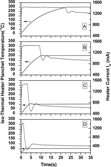
Figure 12. Various set iso-thermal temperature verse heater current generated temperature profile of a developed heater assembly under feedback condition. Here, (A) T = 300 °C, (B) T = 200 °C, (C) T = 100 °C and (D) T = 50 °C.
Download figure:
Standard image High-resolution image3. Results and discussion
Figure 13 shows the typical TL glow curve of CaSO4: Dy Teflon embedded dosimeter (ϕ = 4 mm and 0.8 mm thick) recorded on BOTLR-1 system with a heating rate 3 K s−1 [15]. Other standard TL glow curves have been recorded for the various phosphors such as dosimetric grade 5 mg powder of carbon doped alumina (α-Al2O3:C) [16], Lithium calcium aluminum fluoride doped with europium and yttrium (LicaAlF6:Eu,Y) LCAF [17] as shown in figure 14. The recorded glow curves matches very well with those reported in literature for corresponding phosphors. Once the battery is fully charged, the BOTLR-1 system can record twenty TL readouts with a heating rate of 3 K s−1 up to 400 °C. The typical dynamic dose linearity measured for dosimetric 220 °C TL peak (heating rate of 3 K s−1) for CaSO4:Dy Teflon disc has been shown in the figure 15. A good TL dose linearity of CaSO4:Dy Teflon disc has been observed for applied doses in the range of 0.05 mGy to 1.2 Gy. It must be mentioned here that the selected dose range has great importance in personnel monitoring of radiation workers.

Figure 13. The TL glow curve of the CaSO4: Dy Teflon disc dosimeter recorded on BOTRL-1 with a heating rate of 3 K s−1.
Download figure:
Standard image High-resolution image
Figure 14. TL glow curves (A) LiCaAlF6: Eu, Y and (B) α-Al2O3:C acquired on BOTLR-1 with heating rate of 4 K s−1 for absorbed dose 10 mGy by irradiation with Sr 90 beta source.
Download figure:
Standard image High-resolution image
Figure 15. TL Dose linearity recorded on BOTLR-1 (−900 V applied to PMT) for 220 °C TL peak of CaSO4: Dy irradiated by Sr 90 beta source.
Download figure:
Standard image High-resolution image
The developed miniature dc TL heater assembly is capable of generating the desirable linear heating rates range from 0.1 to 4.0 K s−1, required in most of TL measurements. The considerable agreement between measured and numerically simulated values of (Cm)H for composite heating assembly suggested less impact of insulation material used to fix heater assembly including side screws. The developed theoretical framework will be of great use for designing similar type of miniature heater assembly with the precision heating required for the various scientific experiments. Thus, the developed miniature heater has opened a new possibility of exploring infield use of portable battery operated TL reader systems for radiation measurements.
4. Conclusions
The theoretical model suggested for the heat generation phenomenon in the developed miniature heater assembly has been validated by experimental observation, within the limits of assumed parameter and thermodynamic design. This development has scrutinized the possibilities of designing a compact energy efficient TL reader system for various types of TL based radiation dosimetric applications such as, medical radiology, space dosimetry, nuclear radiological emergency dosimetry etc.
Acknowledgments
This research work is greatly supported by all the members of RPIS/ RP&AD, BARC, Mumbai, India.