
Abstract
Wind power plays a vital role in the global effort towards net zero. A recent figure shows that 93GW new wind capacity was installed worldwide in 2020, leading to a 53% year-on-year increase. The control system is the core of wind farm operations and has an essential influence on the farm's power capture efficiency, economic profitability, and operation and maintenance cost. However, the inherent system complexities of wind farms and the aerodynamic interactions among wind turbines cause significant barriers to control system design. The wind industry has recognized that new technologies are needed to handle wind farm control tasks, especially for large-scale offshore wind farms. This paper provides a comprehensive review of the development and most recent advances in wind farm control technologies. It covers the introduction of fundamental aspects of wind farm control in terms of system modeling, main challenges and control objectives. Existing wind farm control methods for different purposes, including layout optimization, power generation maximization, fatigue load minimization and power reference tracking, are investigated. Moreover, a detailed discussion regarding the differences and similarities between model-based, model-free and data-driven wind farm approaches is presented. In addition, we highlight state-of-the-art wind farm control technologies based on reinforcement learning—a booming machine learning technique that has drawn worldwide attention. Future challenges and research avenues in wind farm control are also analyzed.
Export citation and abstract BibTeX RIS

Original content from this work may be used under the terms of the Creative Commons Attribution 4.0 license. Any further distribution of this work must maintain attribution to the author(s) and the title of the work, journal citation and DOI.
1. Introduction
Wind power is one of the most efficient forms of renewable energy and is critical for the global effort to achieve net-zero emissions and clean growth. It is regarded as the cornerstone of green recovery and is of great significance in the acceleration of global energy transition. Statistics in 2018 indicated that wind power's share of the total power generated by green energy was over one-third, showing that it is currently the most essential renewable source [1]. Tremendous effort has been made to develop wind power and wind farms. The Global Wind Energy Council [2] expects around 94 GW of new wind capacity to be installed annually for the next 5 years. Europe had installed over 220 GM wind power capacity by the end of 2020 [3], which is currently contributing over 15% of the total electricity usage in Europe. In addition, wind power has become an important economic sector in many countries. For example, it adds almost £7bn GVA to the economy and contributes over 30 000 full-time jobs in the UK. Although onshore wind is still in a dominant position in the worldwide wind power capacity, the development of offshore wind has accelerated enormously in recent years, due to its various advantages compared with its onshore counterparts, such as being capable of capturing better wind energy resources with reduced noise influence. Many large offshore wind farms are planned to be put into operation in the next 5 years [3].
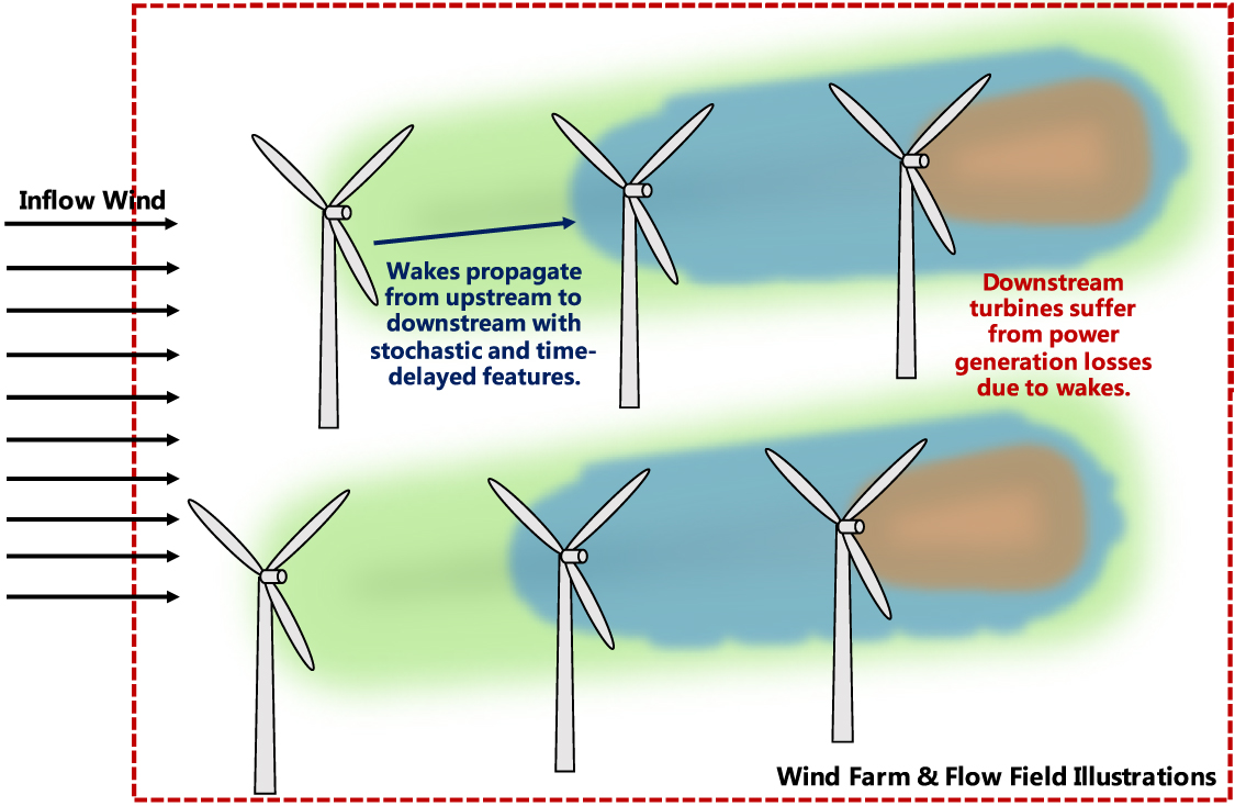
The control system is at the core of wind farm operations and has a critical influence on the power capture efficiency, economic profitability and maintenance cost of wind farms. The enormous growth of both onshore and offshore wind farms imposes various requirements on wind farm control techniques. However, wind farms' inherent system complexities cause significant barriers to control system design. The main challenges in wind farm control come from the strong aerodynamic interactions among wind turbines, complexities related to wind farm modeling, stochastic features of environments, and the enormous amount of data involved in control system design. All these aspects can lead to great influence on the effectiveness, adaptability, robustness and applicability of wind farm optimization and control approaches. Among the most challenging issues is the complex aerodynamic interactions in wind farms, which are induced by wake effects. Specifically, after an upstream wind turbine in the farm extracts power from the inflow wind, its downstream wind flow will be changed, leading to a wake with reduced wind speed and increased turbulence. This wake can lead to the deterioration in the downstream turbines' power extraction process, resulting in degraded control performance. Figure 1 provides a qualitative illustration of the wake effect. It can have a significant influence on wind farm operations. For example, the wake effect is reported to account for a roughly 20% annual power generation loss of Denmark's Horns Rev Offshore Wind Farm [4].

Figure 1. Illustration of a wind farm and wake effects.
Download figure:
Standard image High-resolution imageSubstantial research effort has been made in wind farm control (without loss of generality, in this paper, we regard optimization methods as a special class of open-loop control methods) to address these challenges, and many achievements have been reported with meaningful simulation and experimental results. With the rapid development of wind farms, a review that comprehensively summarizes and analyzes the development of and the most recent advances in wind farm control technologies is needed. This can help researchers and engineers in the wind energy community understand the key needs, pros and cons of existing methods, mainstream and new research trends, and unresolved issues regarding wind farm control, thus promoting this essential research and application area and inspiring next-generation wind farms and other renewable energy technologies. This paper aims to fulfill such a timely need. In particular, a detailed introduction to the requirements and challenges of wind farm operations is provided. This covers the fundamental aspects of wind farm control technologies in terms of system modeling, main challenges and control objectives. Then, we carry out a systematic analysis, evaluation and comparison of existing wind farm control methods. Methods for different purposes, including layout optimization, power generation maximization, fatigue load minimization and power reference tracking, are organized and classified. Moreover, the comparison regarding the differences and similarities between the model-based, model-free and data-driven wind farm control methods is elaborated in detail. In addition, we highlight state-of-the-art wind farm control technologies based on reinforcement learning (RL)—a booming machine learning technique that has drawn worldwide attention. Future challenges and future research avenues in wind farm control are also investigated.
The remainder of this paper is organized as follows. The fundamental aspects of wind farm control are introduced in section 2, including system models, main challenges and essential objectives. Based on different objectives, existing wind farm control approaches are reviewed in section 3, and typical model-based, model-free and data-driven wind farm control methods are considered. Then, the most recent RL-based wind farm control approaches are introduced and analyzed in section 4. Finally, the conclusions and future prospects are given in section 5.
2. Fundamentals in wind farm control: models, challenges and objectives
This section introduces the key aspects that lay the foundation for the control system design of wind farms, including wind farm models, main challenges and main objectives in wind farm control. In addition, historical milestones of wind farm control algorithms are also discussed.
2.1. Wind farm models
Wind farm models are a prerequisite for many wind farm control methods. The majority of mainstream wind farm control approaches are model based. Accurate wind farm models serve as a significant tool to provide key information for wind farm controllers, such as the relationship between the captured power and the wind speed. Wind farm modeling is a challenging yet hot and important research topic [5]. To describe the aerodynamic interactions among turbines, a proper wind farm model should not only consider the dynamics of turbines, but also take into account the dynamics of flow fields. However, due to the complexity of flow field dynamics, wind farm modeling must consider the trade-off between fidelity and computational complexity, which is also an essential issue for model-based control system design. On the one hand, some wind farm models may have high accuracy, but their high computational loads make them difficult for real-time implementation. On the other hand, some models neglect partial dynamics to reduce computational complexity, but this may lead to degraded control performance. Therefore, choosing proper wind farm models is an important issue in the control system design of wind farms. This subsection is dedicated to introducing existing wind farm models, providing potential choices for designing and validating wind farm control methods.
Depending on the fidelity, mainstream wind farm models can be roughly classified into low-fidelity models, medium-fidelity models and high-fidelity models.
Low-fidelity models are usually in steady state. They reflect the time-averaged characteristics of wind farms and flow fields. Although this type of model has less computational complexity, their primary drawback is that they provide few details regarding temporal dynamics, such as wake meandering, leading to limited accuracy. One of the typical and easy-to-implement low-fidelity models is the Jensen model [6]. The Park model was also proposed [7] with further modifications. The U.S. National Renewable Energy Laboratory (NREL) recently developed the so-called FLOw Redirection In Steady-state (FLORIS) model [8], aimed at improving the accuracy of steady-state wind farm models with measurement data. Other examples include the FLORIDyn model [9] and FOWFSim model [8].
Different to low-fidelity models, medium-fidelity models are dynamic and can reflect more flow-field details. However, to reduce computational complexities, medium-fidelity models usually simplify the full Navier–Stokes (NS) equations and ignore some physics. One of the typical medium-fidelity models is the control-oriented Wind Farm Simulator (WFSim) model proposed in [10, 11]. This model was built upon 2D NS equations, neglecting the vertical dimension to reduce the computational time. The idea of system matrix sparsity was employed to further improve the computation efficiency. The turbulence model in WFSim was formulated by the Prandtl's mixing length model, and turbines were described by the actuator disk model. The Ainslie model proposed in [12] was also built upon a simplified NS equation with the assumption of axisymmetric, zero circumferential velocities, and fully turbulent wakes [13]. Other medium-fidelity models include the FarmFlow model [14] and the FAST.Farm model [15].
High-fidelity models usually apply large-eddy simulations (LES) to solve the 3D NS equations with high temporal and spatial densities. They provide high modeling accuracy at the cost of significant computational complexities. One of the most commonly used high-fidelity models is SOWFA (Simulator for Offshore Wind Farm Applications) [16]. SOWFA was formulated with computational fluid dynamics (CFD) tools based on OpenFOAM, and wind turbine models based on the FAST (Fatigue, Aerodynamics, Structures and Turbulence) simulators [17]. It has the ability to accurately reflect flow field changes under varying atmospheric conditions [18]. Another renowned high-fidelity wind farm model is PALM (Parallelized Large-Eddy Model), developed by Leibniz Universitat Hannover [19]. Distinct from SOWFA, which was developed with CFD tools, PALM was formulated with finite element methods and structured staggered meshes [20]. PALM is a Fortran-based code that is parallelized through the decomposition method on a Cartesian grid [19]. Some other high-fidelity models include the SP-Wind model [21] and EllipSys3D model [22].
Some recently developed wind farm modeling methods apply deep-learning techniques to balance fidelity and computational complexity. As an example, a novel dynamic wind farm wake model was designed in [23] via a deep-learning-based reduced-order method. The proposed model has the ability to describe unsteady flow features as high-fidelity wake models while rendering significantly reduced computational complexity similar to the low-fidelity wake models. Zhang and Zhao [24] developed a physics-informed deep-learning-based model for spatiotemporal wind field predictions. It combined LiDAR measurements and flow physics by incorporating a deep neural network (NN) into NS equations.
2.2. Main challenges
One of the critical challenges for wind farm control is the aerodynamic interaction among wind turbines. As demonstrated in figure 1, the power generation of upstream wind turbines results in downstream regions with reduced wind velocity and increased turbulence intensity. This process is commonly referred to as the wake effect, which can influence the power generation process of downstream turbines and the operating efficiency of the whole farm. In addition, the increased turbulence intensity induced by wake effects can lead to fatigue loads in downstream wind turbines [25]. Therefore, it is of paramount importance to consider wake effects in the design of wind farm controllers.
Moreover, the selection of wind farm models is essential in the design of model-based wind farm controllers. As introduced in section 2.1, a trade-off between model fidelity and computational complexity must be made in model selection. The higher the model accuracy, the greater the computational complexity. Some commonly used steady-state models [26] have significantly reduced computational complexity, making them easy to implement in control system design. However, the downside is that these models largely neglect temporal dynamics, which may lead to degraded control performance. However, high-fidelity models have adequate accuracy but suffer from heavy computational costs and poor real-time performance.
The existence of various uncertainties in practice, such as time-varying wind conditions and turbine parameter uncertainties causes another challenge for wind farm control. On the one hand, those uncertainties make it challenging to build an accurate analytical wind farm model [27], which is essential for model-based wind farm controllers. On the other hand, they also lead to difficulties in developing wind farm controllers with strong robustness and adaptability.
Furthermore, with the continuous increase in wind farm scales and number of wind turbines, the measurement data sets in wind farms are becoming larger and larger, which may require excessive computational resources to process and could cause high computational loads. Some data, such as flow field states, are difficult to handle given their time-delayed and distorted features, causing difficulties for the practical deployment of wind farm controllers. Therefore, it is necessary to improve data-processing efficiency in wind farm control system design, particularly for data-driven wind farm controllers.
In addition, wind farm control methods sometimes need to pursue multiple and conflicting objectives subject to various constraints [28], which also causes difficulties with controller design.
All of these aspects render the design of wind farm controllers a highly complicated and challenging task.
2.3. Essential objectives in wind farm control
The fundamental aim of wind farm control is to improve operating efficiency, increase economic profitability and reduce maintenance and operation costs. Considering the above-mentioned challenges, some specific wind farm control objectives are introduced as follows. A comprehensive review of wind farm control methods towards these objectives is given in section 3.
- (a)Wind farm layout optimization: Wind farm layout optimization aims to find the optimal positions for all turbines on a wind farm to maximize the total power production or minimize costs. An objective function usually needs to be constructed with regard to these problems, which should be a function of wind turbine positions and the corresponding objective, such as farm-level power production. These objective functions are commonly based on wind farm models with wake descriptions, such as the Park model [29], which assumes that the wake expands linearly with the wind and moves to the downstream region [30]. Many optimization techniques have been explored for wind farm layout optimization and will be introduced in section 3.1.
- (b)Power generation maximization: In practice, most of the wind farms employ the 'greedy strategy' in power generation. This means that each wind turbine is operated separately to maximize its own power generation [31–33] while ignoring the potential influence on other turbines. However, the greedy strategy is not optimal due to the existence of wake effects. As mentioned, wake effects induced by upstream turbines can significantly influence the power generation of downstream turbines, therefore influencing farm-level power production. Wind turbines on a farm should be cooperatively controlled in order to improve the total power production of the whole farm [34]. This class of wind farm control strategies can be achieved by controlling the axial induction factors and yaw angles of all turbines on the farm [35]. Specifically, adjusting the axial induction factors of upstream wind turbines will lead to decreased momentum and wind-speed deficits of wake [36] in downstream wind turbines, which can potentially increase the power generation of downstream turbines. Consequently, the total power production of the whole farm can potentially be improved. The adjustment of axial induction factors can be achieved by regulating the blade pitch angles, and/or rotor torques of turbines [37]. Another way to mitigate the wake effects is by adjusting the yaw misalignment of upstream turbines to redirect the wakes around downstream turbines [38]. This can decrease the overlapping areas between wakes and downstream turbines, providing downstream wind turbines with higher wind speed and allowing them to generate more power than in the cases without wake re-directions [39].
- (c)Fatigue load minimization: The aerodynamic interactions of wind turbines can cause an increase in turbulence intensity, which can potentially lead to heavy fatigue loads that shorten the lifetime of turbines. Therefore, minimizing fatigue loads is another crucial aspect of wind farm control. It is usually implemented by combining it with power output regulation. For example, [40] solved the fatigue load minimization problem while keeping power production at the desired level.
- (d)Power reference tracking: Modern wind farms are required to perform compatibly to traditional power plants, in order to eventually replace conventional power plants [41, 42]. Therefore, wind farms should meet more rigorous technical requirements and provide auxiliary services to guarantee the safety and operational stability of the power grid. For example, secondary frequency control, as one of the typical auxiliary services, can regulate grid frequency, balance power capture and loads, and maintain power exchanges between areas [43]. To fulfill these requirements, a wind farm's power generation should be capable of tracking a specific power reference generated by transmission system operators in a few to tens of minutes [44]. Some works, such as [42, 45, 46], have shown success with these tasks.
As previously mentioned, these wind farm control tasks aim to improve operating efficiency, increase economic profitability and reduce maintenance and operation costs, and they are the main focus of the discussion in this paper. In addition, many other wind farm control studies considerimportant tasks in the grid integration and transmission network of wind energy. For example, [47] designed an RL-based adaptive wind farm control method to enhance the stability of power systems with wind energy penetration. Dong et al [48] proposed a cooperative control method to maximize the reactive power capacity of network-connected wind farms.
2.4. Historical milestones
To the authors' best knowledge, the first wind farm control strategy was proposed in [34], focusing on improving wind farm dynamic performance. Then, various optimization techniques (in this paper, we regard optimization methods as a special class of open-loop control methods) and closed-loop wind farm control algorithms were developed to achieve different objectives. We briefly depict an illustration in figure 2 to show the development of wind farm control methods. Typical methods include genetic algorithm (GA), evolutionary algorithm (EA), particle swarm optimization (PSO), sequential convex programming (SCP), game-theoretic (GT), random search (RS), model predictive control (MPC), Bayesian ascent (BA) and RL. A detailed introduction to these methods is provided in the following sections.
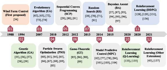
Figure 2. Development of wind farm control methods.
Download figure:
Standard image High-resolution image3. Wind farm control approaches
Given the essential objectives introduced in section 2.3, this section provides a detailed review of existing wind farm control methods.
3.1. Wind farm layout optimization
Wind farm layout optimization aims to determine optimal locations for wind turbines, maximizing the whole farm's power production or minimizing costs while considering various aspects, such as wake effects, wind farm boundaries and wind turbine types [28, 49]. These tasks can usually be formalized as multi-objective nonlinear constrained optimization problems. Various problem formulations and many optimization approaches have been developed to deal with these problems. Typical methods include mixed-integer linear programming [50], ant colony algorithm [51], particle filtering approach [52], lazy greedy algorithm [53], extended pattern search algorithm [54], GA [55–59], PSO [60, 61], RS algorithm [28], SCP [29], EA [62, 63], etc. Typical results are discussed in detail as follows.
To the authors' best knowledge, the first work to tackle the wind farm layout optimization problem was proposed in [55], which utilized GA to obtain candidate solutions. Grady et al [56] also employed GA to optimize wind turbine positions while considering the limitations of wind turbine numbers and land acreage. Moreover, as variants of conventional GA, multi-objective genetic algorithm (MOGA), binary real coded genetic algorithm (BRCGA) and adaptive genetic algorithm (AGA) were developed and applied to wind farms. Specifically, in [57], MOGA was employed to solve a wind farm layout optimization problem. Simulation cases were conducted with commercial turbine parameters and various real wind conditions. Different to conventional GA, the MOGA method proposed in [57] denoted the turbines placement, types and hub heights by mixed discrete strings, which could optimize not only regular wind farm layouts, but also irregular wind farm layouts. Abdelsalam and El-Shorbagy [58] investigated BRCGA for wind farm layout optimization. The position of wind turbines was denoted by the binary part of GA, while the power capture was characterized by the real part of GA. It employed the Jensen wake model. In [59], AGA and self-informed genetic algorithm (SIGA) were designed to optimize the wind farm layout. Specifically, AGA was used to relocate the worst turbine locations, and SIGA was designed to find the optimal locations. In addition, a surrogate model using multivariate adaptive regression was introduced to balance exploitation and exploration, mitigating the disadvantages of conventional GA.
In [64], the PSO method was utilized for the first time to optimize the position of wind turbines, whose efficiency was verified by simulation results. PSO was also investigated in [65] for the same purposes, in which the minimum allowed distance between wind turbines was considered. An improved Gaussian PSO algorithm, combined with a local search strategy, was proposed in [66] to optimize the positions of turbines, which could significantly reduce the execution time. Furthermore, a binary particle swarm optimization with time-varying acceleration coefficients was developed in [67]. In [68], the PSO was applied to solve a wind farm layout optimization problem formulated by the levelized production cost. Pillai et al [69] also employed PSO to handle wind farm layout optimization, and it considered three different levels of wind farm constraints. In [60], a constrained PSO technique was used to solve the unrestricted wind farm layout optimization problem, which was formulated to maximize the power production by optimizing the positions and rotor diameters of wind turbines. Simulation results showed that, compared with an experimental farm, the farm with the optimal layout could achieve an up-to-30% increase in total power generation, and the farm equipped with turbines with different rotor diameters could achieve an up-to-43% rise in total power generation. In [61], the PSO method combined with multiple adaptive methods (PSO-MAM) was designed to solve offshore wind farm layout optimization problems. A restriction zone concept with a penalty function was constructed to solve the limitations of the seabed and marine traffic. Simulation results indicated an increase of 3.84% in power generation was achieved using PSO-MAM compared to the baseline method.
In [70], a refinement method using RS was proposed to find the optimal locations of wind turbines. In [28], an RS algorithm was also designed for wind farms, but it was formulated to minimize the cost of power production considering various constraints. An adaptive mechanism was added to this RS method, with the aim of improving control performance and reducing computation costs. The authors in [71] also utilized an RS algorithm to maximize total power generation and minimize full electrical cable length while considering geographic limitations.
In [29], the SCP technique was used to solve the wind farm layout optimization problem. A continuous wake model was constructed to relate the power function to turbine locations. Then, by determining the gradient and Hessian matrix of the wind farm power function, the SCP method proposed in [29] iteratively found the optimal solution. Simulation results indicate that the method is efficient when applied to a large wind farm with 80 turbines.
An EA method was proposed in [72] for wind farm layout optimization to maximize profits. Another EA method was proposed in [73] for similar purposes, in which a more realistic cost model was designed, allowing the algorithm to consider restricted areas or terrains. Moreover, a multi-objective evolutionary algorithm (MOEA) was proposed in [74] for wind farm applications. This method selected a combination of two turbines from 26 wind turbines with respect to different wind speeds distributed over different time spans. A decomposition-based MOEA/D was developed in [62], in which a set of Pareto optimal vectors was derived for maximizing power generation and improving operating efficiency. To reduce the computational cost, a data-driven EA was designed in [63] to maximize farm-level power generation. In particular, it employed a data-driven surrogate model constructed using general regression NNs, and a fast filtering strategy for potentially bad candidate solutions was employed to improve the optimization efficiency.
In summary, optimization methods for wind farm layout optimization have aroused extensive interest and are widely investigated. Existing techniques can increase farm-level power production and/or reduce costs. Relevant results are validated by extensive simulations.
3.2. Wind farm power generation maximization
In this subsection, we introduce wind farm control methods for farm-level power generation maximization. In terms of model dependency, wind farm control strategies can be roughly divided into model-based and model-free methods. The related works of these two types of methods are discussed in detail as follows.
3.2.1. Model-based methods
Model-based control methods rely on analytical wind farm models to guide control actions, and wake effects should be considered in the control process. Many model-based algorithms have been developed to maximize wind farm power generation. A typical example is the MPC technique, which aims to solve closed-loop optimal control problems with multiple objectives subject to various constraints [75, 76]. A deep neural learning-based predictive control method was developed in [77] to maximize farm-level power generation and minimize control costs. This method was constructed by long short-term memory (LSTM) units combined with convolutional neural networks (CNNs) and MPC methods. They employed CNN-LSTM to predict wind farm outputs based on high-fidelity LES data. Both distributed and decentralized MPC methods were employed to find optimal solutions. Numerical simulations showed that the distributed MPC can achieve a power production increase of up to 38% compared to the decentralized MPC method. In [78], a novel closed-loop model-based wind farm controller was proposed to maximize the power production by adjusting yaw angles. The controller was constructed by estimating surrogate model parameters and carrying out real-time setpoint optimization. A high-fidelity simulation of a six-turbine wind farm was tested to validate the effectiveness of this controller under time-varying inflow conditions. Simulation results showed that this approach could achieve an 11% power gain compared to the benchmark. In [79], a learning model predictive control (LMPC) algorithm was proposed to increase wind farm power production. The LMPC method can learn the state trajectory and input cost based on previous iterations. Its recursive feasibility, stability and convergence analysis were provided. Simulation results showed that the power production could be increased by up to 15% using the LMPC proposed in [79]. In addition to MPC-based methods, many other model-based wind farm control algorithms for farm-level power maximization are introduced as follows.
An SCP method was developed in [80] for wind farm power optimization. A coupling matrix was utilized to provide a simple relationship for wind turbine interactions. Simulations were carried out to demonstrate the efficiency of this SCP method. In [81], SCP was also employed for wind farm cooperative control to maximize power generation. A Gaussian-shaped basis function was used to capture the wind speed information, and a differentiable function was constructed using the control variables as input and the measured power as output. Simulation results with Horns Rev wind farm showed that an increase of around 7% in power generation was achieved by using this SCP technique compared to the greedy strategy.
In [82], a cooperative static GA was designed to improve the power production efficiency of wind farms by controlling the nacelle yaw and blade pitch angles. The steepest descent algorithm was employed to find optimal control actions. Gionfra et al [83] introduced a distributed PSO algorithm based on a cooperative co-evolution technique for wind farm power maximization considering aerodynamic wake effects. This model-based distributed architecture has the potential to rapidly converge to the optimal solution, showing a potential advantage in real-time operations of wind farms. In [84], a receding horizon control was applied to optimize the thrust coefficient of each turbine towards farm-level power maximization, in which gradients were determined by a conjugate gradient method. Case studies indicated that this method increased the total power generation by 7% compared to the greedy strategy.
Note that the above-mentioned model-based wind farm control methods directly utilize analytical models to compute optimal solutions. However, these model-based controllers often suffer from modeling errors and are sensitive to uncertainties, leading to degraded control performance and lack of robustness to real-time changes. Distinct from model-bausingsed wind farm control schemes, data-driven model-based wind farm control methods employ learning mechanisms and system identification tools to approximate wind farm models or utilize measured data to update model parameters. In addition, these methods can potentially carry out model validation and calibration based on the dynamic responses of wind farms instead of employing time-averaged data, as in most of the model-based approaches [85]. We introduce some related works as follows.
Gebraad et al [37] introduced a data-driven model-based method for wind farm power optimization by controlling the yaw angles of wind turbines. A novel parametric model was designed to predict flow velocities and power generation, and its parameters were estimated using data. A GT technique was applied based on this parametric model to find the optimal yaw angles. As a significant extension of [37], another yaw control strategy for farm-level power maximization was proposed in [86]. This controller was designed based on the so-called FLORIS (FLOw Redirection and Induction in Steady-state) model, in which the parameters of this model were estimated by the data generated by SOWFA [18] (a high-fidelity CFD model). Then, a GT approach was applied to FLORIS to optimize yaw angles. Doekemeijer et al [87] proposed a closed-loop model-based wind farm control technique based on a steady-state surrogate model and the Bayesian optimization method. The control strategy was evaluated via simulations, with a wind farm consisting of nine 10 MW DTU turbines. Results showed a 4.4% increase in time-averaged power generation compared to the conventional greedy strategy.
In summary, this section introduces model-based methods for wind farm power generation maximization. Due to the existence of underlying models, model-based methods are relatively easy to implement and can potentially be employed to handle multi-objective tasks under various state and input constraints (e.g. MPC methods). Extensive numerical results have shown that model-based wind farm control methods can lead to better performance than the conventional greedy strategy. A challenge for model-based strategies is that they highly rely on the accuracy of analytical wind farm models. Nevertheless, a mismatch between wind farm models and real physics is inevitable. This mismatch can be caused by many reasons, including uncertainties and modeling errors, time-varying and stochastic wind conditions or other unexpected changes (e.g. actuator faults). These aspects can potentially degrade the control performance and/or reliability. Many studies have been devoted to solving the limitations of model-based methods by investigating model-free alternatives, with the aim of providing better robustness, adaptability and performance. Typical model-free wind farm control methods are introduced in the following subsection.
3.2.2. Model-free methods
Model-free wind farm controllers provide new avenues to deal with the limitations of their model-based counterparts. They are usually driven by measurement data, but without using analytical models. Typically, they aim to iteratively acquire optimal control actions subject to user-defined objective functions or rewards. The literature exploring model-free wind farm control strategies for farm-level power maximization is discussed.
Marden et al [88] explored a GT-based distributed learning algorithm to achieve model-free wind farm control, with the aim of maximizing power production by adjusting axial induction factors. Marden et al [89] also developed a model-free GT method for wind farms, in which a payoff-based distributed learning approach for Pareto optimality was applied. Simulation results showed that the power production under this method can be increased by up to 25% compared to the greedy control.
Zhong and Wang [90] proposed a decentralized model-free optimization approach for power maximization. Two decentralized discrete adaptive filtering techniques were developed based on partial wind farm information. This strategy can lead to a faster convergence rate and lower computational efficiency. Ahmad et al [91] investigated a model-free RS approach. This method was constructed by finding the optimal control parameters for each turbine on the wind farm. The Horns Rev wind farm model was employed to conduct simulations. Ebegbulem and Guay [92] investigated a cooperative time-varying extremum seeking control method for maximizing farm-level power under time-varying wind conditions. A dynamic estimator was used to estimate the cost function, and a parameter estimator was employed to evaluate the gradient.
The BA algorithm was developed in [27, 93–96] to achieve wind farm power generation optimization. It is a data-driven model-free method that only utilizes control variables as inputs and farm-level power generation as output. BA is a probabilistic optimization approach that employs Gaussian regression to approximate the relationship between the system inputs and outputs. In contrast to conventional Bayesian optimization, constraints on the trust region were imposed on the optimization framework of BA, with the aim of monotonically increasing the target value. Simulation results and wind tunnel experiments [94–96] showed the effectiveness of BA. As an extension, [97] proposed a contextual Bayesian optimization method with trust-region (CBOTR) modifications and applied it to wind farms. CBOTR determines the trust region of the next input based on the environmental conditions, with the aim of rapidly finding the next optimal input.
In summary, these works, along with extensive numerical results, demonstrate the effectiveness of model-free methods in farm-level power maximization tasks. They aim to obviate their reliance on analytical wind farm models. One shortcoming is that they are usually open-loop optimization methods that require steady-state data to carry out learning, and they lack adaptability and robustness to time-varying wind conditions and wake effects. How to address these issues is a promising research topic for model-free wind farm control methods.
The architectures of model-based, data-driven model-based and model-free wind farm controllers are illustrated in figure 3, which shows the differences and similarities of these three types of wind farm controllers. Note that data-driven techniques can be applied to both model-based and model-free methods. For data-driven model-based methods, optimal control actions are acquired based on a model approximated/modified by data. For data-driven model-free methods, the optimal control actions are solved by measuring the data directly. Data-driven approaches have the ability to improve the adaptability of wind farm control methods. However, they may suffer from high computational loads by carrying out a large-scale search to find optimal control inputs in a large action space. Data-driven model-based methods can lead to less computational time than fully data-driven model-free methods. This is because they are usually based on parametric models, which can provide smaller or parametric action spaces for finding the optimal control inputs [98]. However, model-free methods potentially have better performance because they are not restricted by underlying analytical models during the learning process.

Figure 3. Main architectures of three different types of wind farm controllers. (a) Model-based wind farm control. (b) Data-driven model-based wind farm control. (c) Model-free wind farm control.
Download figure:
Standard image High-resolution image3.3. Fatigue load minimization and power reference tracking
As previously discussed, one of the main challenges in wind farm control is mitigating the wake effects among wind turbines. Wake effects can increase the downstream turbulence intensity, leading to substantially increased fatigue loads on downstream turbines [25]. These fatigue loads can significantly shorten the service life of wind turbines [99]. Thus, minimizing fatigue loads is essential in wind farm operations. In practice, wind farm controllers are expected to have the ability to dynamically regulate power outputs while minimizing the influence of fatigue loads.
In order to meet more rigorous technical requirements and provide auxiliary services to guarantee the safety and operation stability of the power grid, power reference tracking is another key objective for wind farm control [41]. The power tracking task is a complicated problem because it can have a set of different solutions. For example, the same farm-level power generation can be achieved by derating upstream wind turbines and uprating downstream wind turbines or conversely. Power tracking problems are usually formulated together with other performance indexes, such as reducing control efforts and minimizing fatigue loads. These multi-objective optimal control tasks can be solved by adjusting yaw angles and axial induction factors (determined by thrust coefficients and/or generator torques and/or pitch angles) [100].
Spudić et al [46] explored an optimization-based method for a wind farm to minimize the mechanical load and generate the desired power. A parametric programming strategy was designed to this end. Simulations under different wind speeds showed that this method has the ability to achieve power tracking and load reduction. A distributed MPC (DMPC) approach was explored in [101] for wind farm active power control. DMPC aims to establish a trade-off between wind farm power tracking and load reduction objectives. This could alleviate shaft torque deviation and thrust force change. An extension of the work of DMPC was presented in [42]. Simulation cases under different wind conditions and uncertainties showed that DMPC greatly reduced the mechanical load, while the power tracking performance remained satisfactory compared to centralized MPC algorithms. Yin et al [102] developed a data-driven multi-objective predictive controller (MOPC) using evolutionary optimization for wind farm fatigue load reduction and power maximization. The data-driven predictor was designed with inputs (yaw angles) and outputs (power and fatigue loads) under different wind conditions. The FLORIS model was used to characterize aerodynamic interactions and generate data. Simulation results showed that compared with the traditional MPC method, a thrust load reduction of up to 12.96% was achieved by MOPC, while the power output remained almost the same.
A distributed optimal control method was developed in [40] for minimizing wind farm fatigue loads considering constraints, as well as regulating the power to a given reference. This technique can improve computational efficiency and guarantee asymptotic convergence under certain conditions. Vali et al [45] proposed a closed-loop active power control method for wind farms to track the reference power trajectory and reduce structural loads by controlling axial induction factors. It employed a coordinated load distribution law that regulates the wind turbine power set-points according to feedback measurements. A LES model with a 3 × 4 wind farm was employed to demonstrate this method's effectiveness. Further research into wind farm load reduction was presented in [103], in which wind farms with wake interactions were presented by relevance vector machine (RVM) models. A reliability-aware multi-objective predictive controller was designed based on RVM models, which was solved by meta-heuristic evolutionary algorithms. In [104], a distributed economic MPC approach was developed for large-scale wind farm power tracking and economic optimization. An iterative calculation was employed to realize the Nash optimality. Simulation results with varying wind speed conditions showed that this method can achieve accurate power tracking and reduce fluctuations in pitch/torque.
In conclusion, substantial research effort has been devoted to achieving different wind farm control objectives, including wind farm layout optimization, power generation maximization, fatigue load reduction and power reference tracking. Extensive simulations and experiments have been conducted to validate the effectiveness of existing methods.
Although the important methods mentioned in this section have shown superior performance and advantages over conventional approaches, some essential aspects can be improved further.
- (a)Model-based wind farm control methods commonly suffer from inevitable modeling inaccuracy and stochastic environmental uncertainty. Most of the existing model-based methods for wind farm power generation maximization are open-loop optimization methods. They usually rely on steady-state wind farm models to search for optimal wind farm settings (such as fixed yaw angles and induction factors). Therefore, their adaptability and robustness need to be enhanced.
- (b)Although some model-free approaches have been developed to mitigate the limitations of model-based methods, most of them are still built upon steady-state data (such as time-averaged data or data generated by steady-state models) to carry out learning. These methods still largely neglect the dynamical changes in environmental conditions and wake effects, and it is difficult for them to provide closed-loop control actions based on online measurements subject to time-varying environmental conditions and dynamical wake effects.
- (c)The high system complexity of wind farm dynamics is still a significant barrier to control system design. It is challenging to extract key information from a large measurement data set and maximize long-term rewards for different control objectives.
Aiming to handle these challenges and improve the performance of wind farm operations, some recent works applied RL—a state-of-the-art machine learning technique that has drawn worldwide attention, to wind farm control tasks. A detailed introduction in this regard is provided in the next section.
4. RL-based wind farm control
RL is a cutting-edge machine learning technique and one of the most popular hotspots in artificial intelligence. RL is built upon the trial-and-error principle, with the aim of improving control performance to optimize long-term rewards iteratively. With the help of artificial NNs, which are employed as information processors in RL, this technique can handle high-complexity control problems of 'black-box' systems—problems that are almost impossible to address using conventional control methods. For example, the AlphaGO program [105, 106] developed by Google DeepMind beat the best human players in the board game Go. A key advantage of RL algorithms is that they usually learn the information of systems and the optimal control actions by data or through directly interacting with environments without employing system models.
These features render RL a promising new technique for developing next-generation wind farm control methods. It has the ability to handle the high system complexities and stochastic natures associated with wind farms and flow fields. RL-based wind farm control methods have the potential to mitigate the limitations of model-based wind farm control methods, such as reliance on analytical models and lack of adaptability and robustness to modeling errors and uncertainties. Compared to mainstream model-free wind farm methods that commonly require steady-style data to carry out open-loop optimization, RL-based methods have the ability to handle dynamic measurements and achieve closed-loop control under time-varying environmental conditions. Moreover, they can address some complicated tasks in wind farm operations, such as farm-level power tracking with a reference signal beyond the greedy-mode output, enhancing the task capacity, improving the control performance and promoting the economic profitability of wind farms.
Motivated by the benefits of RL, some studies have been devoted to investigating wind farm control methods by employing/developing various RL algorithms.
4.1. RL overview and problem formulation
The fundamentals of RL are briefly introduced in this subsection. Then, we show an example of molding wind farm control problems into the RL framework.
4.1.1. Fundamentals of RL
There has been a dramatic increase in interest in the RL technique in recent years. It can deal with black-box optimization and control problems without knowing the complete structure of the system. It can extract the core information of systems through data/measurements to achieve multiple tasks [107–109]. RL techniques have made great contributions to a wide range of fields, such as the control problems of robots [110], spacecraft [111] and autonomous vehicles [112]. In addition, some studies have applied RL methods to wind turbine control [113–117]. RL has also been successfully applied to many aspects related to renewable energy system operations, such as energy storage management [118, 119], power system stabilization [120], frequency control [121], wind energy scheduling [122, 123] and system maintenance [124, 125].
An RL agent is usually modeled as a Markov decision process (MDP) [126]. MDP is commonly described by a tuple ![$[s_t,a_t,r_t,M,\gamma, \pi]$](https://content.cld.iop.org/journals/2516-1083/4/3/032006/revision3/prgeac6cc1ieqn1.gif) , where
, where  is the current state at time t,
  is the action,
  is the reward, and S, A and R denote the state, action and reward spaces, respectively. M denotes the transition process with the form of
  , which determines the probability of transitioning to the next state
  when the current state st
and action at
are given. Note that
when the current state st
and action at
are given. Note that  only depends on its immediate past st
and the action at
. Moreover,
only depends on its immediate past st
and the action at
. Moreover, ![$\gamma \in [0,1]$](https://content.cld.iop.org/journals/2516-1083/4/3/032006/revision3/prgeac6cc1ieqn8.gif) is a discount factor that balances immediate and future rewards, and π denotes the policy mapping from the state s to the action a.
is a discount factor that balances immediate and future rewards, and π denotes the policy mapping from the state s to the action a.
A single loop for an RL agent to interact with the environment is as follows. At any time step t, the agent has a state st
and takes a candidate action at
. Then, it receives a reward rt
from the environment and is transferred to a successor state  . The goal of RL is to learn an effective policy
  to maximize the long-time reward
  , where
  indicates the instantaneous reward at st
after taking the action at
.
indicates the instantaneous reward at st
after taking the action at
.
It is noteworthy that many wind farm control tasks are originally partial-Markov processes due to the stochastic nature of environmental conditions and the time-delayed feature of wakes. This issue can be mitigated by properly setting/designing states, rewards and actions, therefore transforming partial-Markov decision problems into Markov decision problems. Based on the requirements of different control objectives, many studies have addressed this issue via different designs/settings. For example, [127] formalized the problem of STATCOM-ADC (static synchronous compensator with additional damper controller) parameter settings under stochastic environments as a Markov decision process, and tested the performance of their RL-based controller with simulations based on an actual wind farm in China. Dong et al [128, 129] employed regulated power generation outputs under different wind conditions to mitigate the partial-Markovian feature in farm-level power maximization tasks, and [43] addressed this issue by utilizing time-series data to form the MDP for wind farm power tracking tasks.
4.1.2. Problem formulation
In this subsection, we demonstrate an example of how to mold the wind farm control problem into an RL framework. For simplicity, we employ a commonly used RL structure and consider a typical wind farm description. What we are showing here is an easy-to-follow example among various possible application forms of RL in wind farm control.
Based on the actuator disk theory [130], the force and power generated by each turbine on a wind farm can be represented in the following two equations, respectively:


Here,  , and N is the total number of wind turbines. Ad
is the area of the rotor plane, Ui
is the wind speed, φi
is the yaw angle, αi
is the axial induction factor,
, and N is the total number of wind turbines. Ad
is the area of the rotor plane, Ui
is the wind speed, φi
is the yaw angle, αi
is the axial induction factor,  is the thrust coefficient and
  is the power coefficient.
  and
and  satisfy:


where µ is a constant parameter. The total power production of the wind farm can be defined as:

It should be emphasized that equations (1)–(4) from the actuator disk theory are actually not indispensable for the applications of RL in wind farm control. Here, they only aim to provide insight into the physical relationships of key wind farm states. The relationship of αi , φi and Ui with Pi can be a 'black box' in RL-based wind farm controllers, i.e. the h function in the following equation can be unknown to the RL agent:

The tasks of wind farm power generation maximization, fatigue load reduction and power reference tracking can be achieved by controlling the yaw angle φi
and axial induction factor αi
of each wind turbine on the farm. Without loss of generality, the power/thrust coefficient, torque or pitch can alternatively be adjusted to control the induction factor. Moreover, the control inputs can be selected to be yaw angles, induction factors or other related variables, such as their increments, changes and error values. Considering wind turbine physics, the control inputs can also be rotor torques and pitch angles. For simplicity, here we set yaw angles and axial induction factors as control inputs, denoted as ![$a_t = [\alpha_{1_t},\ldots,\alpha_{N_t},\phi_{1_t},\ldots,\phi_{N_t}]^\textrm{T}$](https://content.cld.iop.org/journals/2516-1083/4/3/032006/revision3/prgeac6cc1ieqn18.gif) .
.
Based on these preliminaries and assumptions, we set the goal of RL to find an optimal control policy ![$a^*_t = [\alpha^*_{1_t},\ldots,\alpha^*_{N_t},\phi^*_{1_t},\ldots,\phi^*_{N_t}]^\textrm{T}$](https://content.cld.iop.org/journals/2516-1083/4/3/032006/revision3/prgeac6cc1ieqn19.gif) to maximize the long-time reward formalized in (7):
to maximize the long-time reward formalized in (7):

where kp
, kf
and kh
are user-defined weighting constants to balance different tasks. In (7), the first term  denotes a function related to the farm's total power generation. The second term
  is related to fatigue load reduction tasks, which is a function of wind farm states and actions. The third term
  is a function of the error between the total power production and the reference power Pref, which is used to achieve power reference tracking. Therefore, by choosing different values for kp
, kf
and kh
, equation (7) can represent different control tasks. For example, the case where
is a function of the error between the total power production and the reference power Pref, which is used to achieve power reference tracking. Therefore, by choosing different values for kp
, kf
and kh
, equation (7) can represent different control tasks. For example, the case where  ,
,  and
and  indicate a pure power maximization task.
A typical RL structure for solving the optimal control problem indicated by (7) is the actor-critic framework, which is demonstrated in figure 4. Here, the critic NN evaluates the complicated reward functional Rt . The actor NN derives the optimal control action based on the estimated reward functional. All the studies that are introduced in the following subsection are based on this RL framework or its variants.

Figure 4. Typical RL structure for wind farm control.
Download figure:
Standard image High-resolution image
4.2. Applications of RL in wind farm control
This subsection highlights the existing works that developed RL-based methods for wind farm control problems.
4.2.1. Power generation maximization via RL
In recent years, different RL-based approaches have been developed to handle wind farm power maximization tasks, with the aim of achieving superior performance than mainstream methods.
Many RL-based wind farm control methods are based on the Q-learning algorithm [131]. A decentralized Q-learning algorithm was developed in [132] for optimizing farm-level power production. This scheme has the ability to avoid sharp changes in control variables. In [133], a distributed RL algorithm was proposed to increase power generation by controlling yaw angles. In particular, the delay in wake propagation and the stepwise-varying inflow conditions were considered in this study. Another wind farm control method based on the Q-learning algorithm was proposed in [134], in which the idea of gradient approximation of RL and incremental comparison (GARLIC) was constructed for solving the optimal control actions. Simulation tests of these studies showed that RL-based wind farm control methods can achieve improved performance compared to other commonly employed methods. However, a drawback of the Q-learning framework is that the action space must be discrete. Other RL algorithms have been developed for wind farm applications to address this issue and handle more general wind farm control problems with a continuous action space.
Dong et al [128] developed an RL-based wind farm control architecture by combining the deep deterministic policy gradient (DDPG) algorithm with a reward regularization module (RRM) and a composite learning-based control strategy. In particular, RRM was used to normalize the changes in power generation under different wind conditions. The high-fidelity simulator SOWFA [18] was employed to conduct numerical tests, showing that an increase of up to 15% in total power generation can be achieved with this method. In [129], another RL method with improved learning efficiency was proposed and applied to wind farm control. In particular, a composite experience replay (CER) strategy was designed to balance rewards and temporal difference errors during the learning process. CER-RL has better sampling and learning efficiency than mainstream RL methods, enhancing its applicability to practical wind farms.
The RL-based wind farm control methods in [128] and [129] employed yaw angles as control inputs. As an extension study, [135] explored a double-network-based DDPG approach that considered both yaw angles and induction factors as control signals to enhance flexibility and improve control performance further. A key design is that two sets of actor-critic networks were constructed to generate control policies for induction factors and yaw angles simultaneously and separately. This allowed DN-DDPG to deal with the incompatibility between different control signals, ensuring a reliable training process. Another RL-based wind farm control method, called the knowledge-assisted deep deterministic policy gradient (KA-DDPG) method, was proposed in [136]. KA-DDPG also employed both yaw angles and induction factors as control inputs. The key idea of KA-DDOG is to accelerate the learning process by employing analytical models to initialize the RL agent and guide it in the early stage.
4.2.2. Power reference tracking via RL
In addition to power generation maximization, RL can also be applied to handle many other complex tasks in wind farm operations, such as farm-level power tracking, with the aim of providing ancillary services such as frequency regulation.
Wind farm power tracking is a relatively more challenging task than power maximization because the former requires tracking a time-varying reference input. In addition, in this tracking task, real-time control signals can have a long-term and time-delayed impact on the aerodynamic interactions of wind turbines and the power generation of the whole wind farm [43], which should be considered in control system design to optimize performance. Conventional wind farm power tracking methods usually ignore these aspects. Moreover, conventional methods carry out power tracking by de-rating turbines. This means they can only track references below the power curve under the greedy strategy. RL's strong information extraction and learning abilities address these limitations and achieve better task capacity and control performance. Some of the most recent works have investigated this interesting topic.
Vijayshankar et al [137] explored a deep RL framework for wind farm power tracking, which is a model-free method and can solve the optimal actions in real time considering varying environmental conditions. The FLORIS model was employed to conduct numerical simulations. Dong and Zhao [43] designed a preview-based robust deep RL (PR-DRL) for the same purpose. PR-DRL is also data driven and model free. It is based on the  control technique, leading to solid robustness against stochastic environmental conditions. In addition, by employing time-series data for NN training, PR-DRL addresses the short-sighted issue of conventional wind farm power tracking methods and tracks non-trivial references that are higher than the greedy-mode power curve.
The existing RL-based wind farm control methods show the feasibility of employing RL to handle challenging tasks in wind farm operations and achieve improved performance in multiple tasks, including farm-level power maximization and tracking. Table 1 summarizes the features and control performance of these existing RL-based wind farm control methods, where we identify the efficiency gains obtained through comparison with the conventional greedy strategy.
Table 1. Key features of existing RL-based wind farm control methods.
| Reference | Method | Objective | Control input | Simulator | Efficiency gain |
|---|---|---|---|---|---|
| [136] | KA-DDPG | Power maximization | Induction factor | WFSim | 10% |
| [129] | DDPG | Power maximization | Yaw angle | WFSim | 25% |
| [128] | DDPG | Power maximization | Yaw angle | SOWFA | 15% |
| [135] | DN-DDPG | Power maximization | Thrust coefficient and Yaw angle | WFSim | 33% |
| [43] | PR-DRL | Power tracking | Thrust coefficient and Yaw angle | WFSim | — |
| [133] | Distributed RL | Power maximization | Yaw angle | FLORIS | 8.2% |
| [137] | Deep RL | Power tracking | Yaw angle | FLORIS | — |
5. Conclusions and future prospects
5.1. Conclusions
This paper reviews the development and most recent advances in wind farm control technologies. We introduce fundamental aspects of wind farm control regarding system modeling, main challenges and control objectives. Then, existing wind farm control methods for different purposes, including layout optimization, power generation maximization, fatigue load minimization, and power reference tracking, are reviewed and analyzed. Discussion regarding the differences and similarities between model-based, model-free and data-driven wind farm control methods is provided. In addition, the application of RL techniques in wind farm operations is highlighted. The following are some key observations.
- (a)Various optimization techniques have been developed for wind farm layout optimization. They mainly focus on adjusting the positions of wind turbines to maximize power production and minimize costs. Typical methods include PSO, RS, GA, SCP, etc.
- (b)The majority of wind farm control tasks require direct adjustments in wind turbine states. Relevant tasks considered in this paper include power generation maximization, fatigue load minimization and power reference tracking. Existing wind farm control approaches for these tasks can be roughly divided into model-based and model-free methods. The former are developed directly based on analytical wind farm models. They are relatively easy to implement and can deal with multi-objective tasks under various constraints. A downside of model-based approaches is that they are sensitive to uncertainties and modeling errors and lack adaptability and robustness to stochastic environmental conditions. Model-free methods aim to obviate the reliance on analytical wind farm models. They employ measurement data to carry out learning and find optimal solutions. Many results have demonstrated that model-free approaches have the ability to achieve superior performance compared to their model-based counterparts. However, these important methods still have limitations. One example is that most model-free strategies for farm-level power maximization are still built upon steady-style data (such as time-averaged data or data generated by steady-state models) to carry out learning.
- (c)Due to the various merits of the RL technique, including the ability to handle high system complexities, data-driven and model-free features, and strong adaptability, attempts to apply RL to wind farm control tasks have been made in recent years. Results show that RL-based wind farm control methods have the potential to achieve enhanced performance in many tasks, such as power maximization and tracking. On the one hand, they can mitigate the limitations of model-based wind farm control methods, such as reliance on analytical models and lack of adaptability and robustness to modeling errors and uncertainties. On the other hand, compared to the mainstream model-free wind farm methods that commonly require steady-style data to carry out open-loop optimization, RL can handle dynamic measurements and achieve closed-loop control under time-varying environmental conditions.
5.2. Future prospects
Although existing wind farm control methods have shown effectiveness in multiple tasks, many aspects still need further improvements in future research to promote the development of wind farm control technologies. We name a few here.
- (a)Handling the stochastic nature of environmental conditions (such as time-varying wind speeds and wind directions) is still challenging for wind farm control. Although some methods, especially RL-based wind farm control methods, have a certain level of robustness in this respect, their robustness is still limited. Most existing wind farm control methods cannot deal with rapid wind direction changes. In addition, ensuring robustness and safety under extreme environmental conditions remains a research gap.
- (b)The computational complexity of many existing wind farm control methods increases exponentially with the increase in the number of wind turbines. Therefore, how to reduce computational costs is another important research topic. A potential solution is to apply grouping strategies for large-scale wind farms, dividing the whole wind farm into small sub-groups based on the aerodynamic interactions among turbines. This can potentially reduce the algorithm complexities from exponential to linear. Although some attempts have been made to this end, a systematic result is still lacking.
- (c)Due to the diversity of task requirements, it is common for wind farm controllers to pursue multiple (or even conflicting) objectives. Existing methods usually achieve this by designing simple weighted objective functions. More practical objective functions that can fully reflect the trade-off between different objectives from an economic perspective are needed. This will be beneficial for improving the generality of wind farm control methods.
Data availability statement
The data that support the findings of this study are available upon reasonable request from the authors.
Acknowledgment
This work has received funding through the UK Engineering and Physical Sciences Research Council (Grant No. EP/S000747/1).