

Abstract
We present the idea and illustrate potential benefits of having a tool chain of closely related regular, unscreened and screened hybrid exchange–correlation (XC) functionals, all within the consistent formulation of the van der Waals density functional (vdW-DF) method (Hyldgaard et al (2020 J. Phys.: Condens. Matter 32 393001)). Use of this chain of nonempirical XC functionals allows us to map when the inclusion of truly nonlocal exchange and of truly nonlocal correlation is important. Here we begin the mapping by addressing hard and soft material challenges: magnetic elements, perovskites, and biomolecular problems. We also predict the structure and polarization for a ferroelectric polymer. To facilitate this work and future broader explorations, we present a stress formulation for spin vdW-DF and illustrate the use of a simple stability-modeling scheme. The modeling supplements density functional theory (DFT) (with a specific XC functional) by asserting whether the finding of a soft mode (an imaginary-frequency vibrational mode, ubiquitous in perovskites and soft matter) implies an actual DFT-based prediction of a low-temperature transformation.
Export citation and abstract BibTeX RIS

Original content from this work may be used under the terms of the Creative Commons Attribution 4.0 licence. Any further distribution of this work must maintain attribution to the author(s) and the title of the work, journal citation and DOI.
1. Introduction
Modern density functional theory (DFT) calculations seek to describe general matter, ideally with one and the same exchange–correlation (XC) energy functional for all materials, i.e., under a general-purpose hat. Truly nonlocal and strong correlation effects, as well as truly nonlocal (Fock) exchange, play important roles in many systems, where different interaction components compete [1–7]. Some challenges come from the tendency to overly delocalize orbitals in regular, that is, density-explicit functionals, and some from the need to handle strong (local) correlation. These problems can be ameliorated by inclusion of a fraction of Fock exchange in so-called hybrid XC functionals [8–15] or by inclusion of a Hubbard term, in so-called DFT + U [16]. A further long-standing challenge for DFT is a proper and balanced inclusion of van der Waals (vdW) forces [2, 7, 17–25].
It is expected that, at least for now, one must retain both a regular (density-explicit) XC functional, a hybrid XC functional, as well as an option for a Hubbard-U correction in DFT calculations [6]. However, it is also desirable to limit the personal DFT tool box to essentially two or three fixed XC choices of related origin. This is because one can then more easily compare DFT results among different types of materials and more easily gather experience to seek further development [6, 25, 26]. For example, a popular choice is to use XC functionals that originate from the constraint-based formulation of the generalized gradient approximation (GGA) [27–32], by picking PBE [33] as the regular functional, PBE0 [9, 11] as an unscreened hybrid, and HSE [12] as the range-separated hybrid (RSH) that also secures a screening of the long-range Fock-exchange component. This XC tool-chain works when the impact of truly nonlocal-correlation effects can be ignored.
The van der Waals density functional (vdW-DF) method [4, 13, 17, 25, 26, 34–38] has a systematic inclusion of truly nonlocal correlation effects. Moreover, as of very recently [15], it also provides an XC tool chain of closely related consistent vdW-DF [25] XC functionals. That is, the method now has the consistent-exchange vdW-DF-cx [4, 26, 38] (here abbreviated CX) as a current-conserving density-explicit XC starting point, the zero-parameter vdW-DF-cx0p [13, 14] (here abbreviated CX0P) as an associated unscreened nonlocal-correlation hybrid, and the new vdW-DF-ahcx [15] (here abbreviated AHCX) RSH hybrid form. These forms are deliberately kept free of adjustable parameters.
The vdW-DF method and our consistent-vdW-DF tool chain include a balanced density-based account of vdW forces, starting from the screening insight that reflects the design of semilocal functionals [4, 15, 22, 25, 26, 38, 39]. It places all of the competing interactions on an equal ground-state DFT foundation, as all terms directly reflect the variation in the ground state electron density n(r). This is true also for CX0P and AHCX, because they use the Kohn–Sham (KS) orbitals of the underlying density-explicit CX functional in the Fock-exchange evaluation [25, 26]. Moreover, the Fock-exchange mixing in CX0P [14] and (by extension) in AHCX [15] is set from an analysis of the coupling-constant scaling analysis of the correlation-energy term [40], which again is completely specified by the electron density variation [14].
In this paper, we illustrate the general-purpose usefulness of the consistent-vdW-DF XC tool chain (CX/CX0P/AHCX), and we begin work to expand their use for magnetic systems. That is, we provide a formulation of stress in spin vdW-DF calculations [38] and implement it in the planewave-DFT software suite QUANTUM ESPRESSO [41, 42]. We also illustrate an approach to elucidate stability in the presence of soft modes, i.e., vibrational modes that have an imaginary frequency when described in a quadratic approximation to the potential energy variation with local deformations. Our approach is inspired by a quantum theory of temperature variations of polarization fluctuations above the ferroelectric transition temperature [43]. We combine Landau-expansion theory [44] with inelastic resonant tunneling [45–50] for a simple, but generic, discussion of materials characterizations in the presence of soft modes.
Accurate determinations of spin and vibrational effects are central requirements for the usefulness of the vdW-DF method. A proper spin-vdW-DF formulation for the XC value  and for XC-potential components,
  is generally needed to accurately describe the atoms, and hence bulk cohesion [51]. Moreover, we need spin in many materials directly, for example, in magnetic elements and perovskites. For such problems it is desirable to have access to spin-vdW-DF stress results to enable consistent structural optimizations. Similarly, vibrations often directly affect and will at least fine tune material characterizations, as some of us have explicitly demonstrated for transition-metal and perovskite thermophysical properties [51–55].
A broad test, from hard to soft matter, of usefulness of the consistent-vdW-DF tool chain is needed. Structure, polarization, and vibrations are seen as strong discriminators of DFT performance as they directly reflect the electronic structure variation [4, 25, 56–58]. The CX/CX0P/AHCX demonstration and testing goal is pursued by computing material properties using at least two parts of the tool chain (as relevant and possible). We characterize magnetic elements' structure and cohesion, structure in a ferromagnetic perovskite, as well as the elastic response, vibrations, and phase stability in the nonmagnetic SrTiO3. The latter has a known phase transition and offers an opportunity for contrasting with BaZrO3, which remains cubic all the way down to zero temperature [54, 55]. We furthermore study biomolecular test cases and intercalation in DNA to document that CX is accurate for soft matter, and proceed to predict the structure and polarization response in the ferroelectric polyvinyl-di-fluoride (PVDF) polymer crystals.
The paper is outlined as follows. In section 2 we present theory, including a formulation of stress calculations in spin vdW-DF. Section 3 contains an overview of computational methods. Sections 4–6 address a number of challenges, from hard to soft, that we study and discuss to validate the theory contribution and to illustrate use of the consistent-vdW-DF tool chain. Finally, section 7 contains an overall discussion and a summary while appendices
2. Theory
The vdW-DF method is in general well set up as a materials theory tool. It is, for example, implemented in broadly used DFT code packages such as QUANTUM ESPRESSO [41, 42], VASP [59, 60], WIEN2K [61, 62], CP2K [63, 64], as well as in GPAW [65, 66] and OCTOPUS [67–69] through our LIBVDWXC library [70]. The code packages come with a full set of vdW-DF versions and variants.
In some code packages the spin effects on energies, forces and stress are approximated by setting the nonlocal correlation terms without attention to spin impact on the underlying plasmon-dispersion model. This is not so in our implementation of spin vdW-DF [38] in QUANTUM ESPRESSO (that also has spin versions of CX, CX0P, and AHCX). The code permits users to check if there are relevant spin vdW-DF effects to consider in their system of interest, for example, in the description of bulk cohesion and molecules [15, 51]. However, to fully benefit from this QUANTUM ESPRESSO status, we need to enable variable-cell calculations by providing also a stress description for spin vdW-DF.
2.1. Spin vdW-DF calculations
The vdW-DF method is a systematic approach to design XC functionals that capture truly nonlocal correlation effects. Pure vdW interactions (produced by electrodynamic coupling of electron–hole pairs [25, 31, 39, 71, 72]) are examples of nonlocal-correlation effects. Another example is the screening (by itinerant valence electrons) that shifts orbital energies as, for example, captured in a cumulant expansion [73]. In the vdW-DF design we note that both are reflected in an electrodynamics reformulation of the XC functional [25]. This allows us to treat all XC effects on the same footing in the electron-gas tradition.
In practice, we use a GGA-type functional  to define an effective (nonlocal) model of the frequency-dependence of the electron-gas susceptibility α(ω). For reasons discussed elsewhere [22, 36, 39], we limit this input to local-density approximation (LDA) plus a simple approximation for gradient-corrected exchange. We formally express the internal semilocal functional
  as the trace of a plasmon propagator SXC(
r
,
r', ω),
as the trace of a plasmon propagator SXC(
r
,
r', ω),

The trace is here taken over the spatial coordinates of SXC(
r
,
r'; ω). The term Eself denotes an infinite self-energy that removes the formal divergence. For spin-carrying systems we work with the spin-up and spin-down density components ns=↑,↓(
r
) of the total electron density n(
r
) = n↑(
r
) + n↓(
r
). The spin polarization η(
r
) = [n↑(
r
) − n↓(
r
)]/[n↑(
r
) + n↓(
r
)] impacts the GGA-type internal functional  , and must therefore be directly reflected in the details of the plasmon propagator SXC(
r
,
r', ω) [38].
, and must therefore be directly reflected in the details of the plasmon propagator SXC(
r
,
r', ω) [38].
The key point is that the model plasmon propagator SXC also defines an effective GGA-level model dielectric function  (iu) = exp(SXC(iu)) and a corresponding model susceptibility α(iu) = ((iu) − 1)/4π. Moreover, by enforcing current conservation, the dielectrics modeling also defines the full vdW-DF specification of the XC functional,

where G denotes the Coulomb Green function. By expanding equation (2) to first order in SXC, one formally recoups the internal GGA-type functional equation (1). By further expanding to second order, we obtain the vdW-DF determination of corresponding nonlocal-correlation effects,

As indicated by superscript 'sp', the nonlocal-correlation term depends on the spatial variation in the spin polarization η( r ) through SXC( r , r'; ω) [38].
Functionals of the vdW-DF family are generally expressed as

where  contains nothing but LDA and the gradient-corrected exchange while
  is the nonlocal-correlation term. The Lindhard–Dyson screening logic formally mandates that the cross-over exchange term
  must vanish, thus setting the balance between exchange and correlation [25]. There are, however, practical limitations that prevent us from going directly for such fully consistent implementations. In the consistent-exchange vdW-DF-cx version we have chosen
  so that the nonzero cross-over term does not affect binding energies in typical bulk and in typical molecular-interaction cases, as discussed separately in references [4, 25, 26, 74].
For actual evaluations, we use a two-pole approximation for the shape of the plasmon-pole propagator SXC. This plasmon-pole description, and hence the resulting vdW-DF version, is effectively set by the choice of the semilocal internal functional EXC via equation (1). This leads to the computationally efficient nonlocal-correlation determination

where D = | r − r'|. It is given by a universal kernel form Φ, as discussed in reference [75]. In equation (5), the values of q0( r ) and q0( r') characterize the model plasmon dispersion.
The above-summarized vdW-DF framework leaves no ambiguity about how to incorporate spin-polarization effects in  . Spin enters via the exchange and via the LDA-correlation parts of
  , as given by the spin-scaling description and by the now-standard PW92 formulation of LDA [76]. This, in turn, determines the form of SXC and ultimately equation (5). Specifically, the values of q0(
r
) and q0(
r') are set from the local energy density of the internal semi-local functional to reflect the density and spin impact on the underlying screening description. Of course, it is imperative to also include spin in the
, as given by the spin-scaling description and by the now-standard PW92 formulation of LDA [76]. This, in turn, determines the form of SXC and ultimately equation (5). Specifically, the values of q0(
r
) and q0(
r') are set from the local energy density of the internal semi-local functional to reflect the density and spin impact on the underlying screening description. Of course, it is imperative to also include spin in the  term. This proper spin vdW-DF formulation [38] is implemented in QUANTUM ESPRESSO [41, 42] and in the LIBVDWXC library [70], permitting fixed-cell calculations but not (until now) general variable-cell vdW-DF studies.
2.2. The nonlocal-correlation stress tensor
For non-spin-polarized problems, there has since long existed a formulation of stress in vdW-DF calculations [77]. This allows effective KS structure optimizations as implemented in QUANTUM ESPRESSO. We now present a spin vdW-DF extension of stress to enhance the KS-structure search part. It is based on the ideas of Nielsen and Martin [78] and we first summarize the non-spin vdW-DF stress calculations, as derived by Sabatini and co-workers [77]. We consider the impact of unit-cell and coordinate scaling, for example, as expressed in Cartesian coordinates for a position vector  , where ɛα,β
is the strain tensor. This scaling affects the double Jacobian, the total-electron density n(
r'), the total-density gradient ∇n(
r
) and the coordinate-separation variable D inside Φ in equation (5). Details of these different scaling effects are discussed in appendix
, where ɛα,β
is the strain tensor. This scaling affects the double Jacobian, the total-electron density n(
r'), the total-density gradient ∇n(
r
) and the coordinate-separation variable D inside Φ in equation (5). Details of these different scaling effects are discussed in appendix
In the absence of spin polarization, Sabatini and co-workers [77] derived the nonlocal-correlation stress tensor contribution

where

and

This stress component is in part given by the nonlocal-correlation contributions,  and
and  , to the XC potential and XC energy. These contributions are given by local values of an inverse length scale, q0(
r
), that determines the local plasmon dispersion. As such, the contributions depend on the density gradients and hence have an indirect dependence on coordinate scaling, as summarized in equation (8).
, to the XC potential and XC energy. These contributions are given by local values of an inverse length scale, q0(
r
), that determines the local plasmon dispersion. As such, the contributions depend on the density gradients and hence have an indirect dependence on coordinate scaling, as summarized in equation (8).
For stress evaluations it is important to note that the density gradient will scale both since the density scales with the unit-cell size and because the formal expression for the spatial gradient scales with coordinate dilation even at a fixed density. The former effect is incorporated by the term containing  . The latter effect is captured by the term in the last row of equation (6). Fortunately, the local variation of q0 is already computed as part of any self-consistent (spin) vdW-DF calculation.
The internal functional depends on the variation in the spin polarization η(
r
) and this spin dependence impacts the plasmon dispersion, and ultimately  , through the local q0(
r
) values. To also compute stresses in spin vdW-DF we must update equation (6) accordingly; details are discussed in appendix
, through the local q0(
r
) values. To also compute stresses in spin vdW-DF we must update equation (6) accordingly; details are discussed in appendix
We find that the second line of equation (6) only changes to the extent that the values of the q0's must now be evaluated for η( r ) ≠ 0. For the first line, there is a small modification since separate XC potentials now act on n↑( r ) and n↓( r ).
Finally, for an update of the third line of equation (6), we simply track the variation of the local q0 values on both spin-density gradient terms. Thus, the resulting spin-vdW-DF stress tensor expression becomes

where

As in the non-spin-polarized case, the spin vdW-DF stress contribution, equation (10), is conveniently given by quantities that are already computed in a self-consistent determination of the electron density variation in spin vdW-DF.
Sabatini et al [77] incorporated their non-spin stress result in the QUANTUM ESPRESSO DFT code suite. We have now completed a full spin vdW-DF implementation by having already contributed our spin-vdW-DF-stress code extension to this open-source DFT suite. Our public release makes a previous work-around (available through a compiler flag) obsolete in QUANTUM ESPRESSO: users no longer have to omit the spin impact on the evaluation of the nonlocal-correlation energy term when performing variable-cell vdW-DF calculations in spin-polarized systems.
2.3. Functional tool chains with semilocal and with truly nonlocal correlation terms
We use and compare results obtained in PBE- and CX-associated hybrids, both unscreened and in an RSH form. We see these functionals as tool chains of closely related functionals, having either a semilocal or a truly-nonlocal correlation term. The former tool chain comprises PBE [33], PBE0 [9, 11], and HSE [12]. The latter tool chain is defined by consistent vdW-DFs [25] and is new. It comprises CX [4, 26], CX0P [14], and AHCX [15].
The PBE0 [9, 11, 13] is an unscreened hybrid based on PBE. One merely replaces 25% of the PBE exchange component with an evaluation based on the KS orbitals. The HSE functional [12] is an RSH extension of the PBE functional. We use it with 25% Fock exchange and a range separation that is described by a screening parameter μ = 0.2 Å−1. This parameter defines an error-function weighting erf(μr)/r of the Coulomb interaction [12], thus limiting the Fock-exchange inclusion to short separations.
The vdW-DF-cx0 is an unscreened hybrid class that is formulated in analogy with PBE0 [9, 11, 13] but starting instead with CX. We use the zero-parameter form CX0P [14] in which the extent of Fock exchange mixing is kept fixed at 20%, following an analysis of the CX coupling-constant scaling [40] that enters the general hybrid design logic [11, 14].
Finally, the AHCX is the recently launched CX-based RSH [15]. It resembles the CX0P in that we keep the Fock exchange fraction fixed at 20% and it resembles HSE in that we keep the screening parameter fixed at the standard HSE value [12]. The screening makes AHCX calculations relevant for metallic systems [15].
3. Computational methods
In total, 15 different functionals were used for our calculations, although half of those were exclusively used to establish an impression of present status for performance on benchmarks of biomolecular relevance. For this test, we leverage the full range of nonlocal-correlation functionals in the new, consistent-vdW-DF tool chain and we compare with vdW-DF1 [17] and vdW-DF2 [37], other members of the vdW-DF family of nonlocal-correlation functionals [79–84], as well as results obtained by using revPBE + D3 [33, 85, 86] and HSE + D3 [12, 86]. The revPBE + D3 functional is considered one of the very best overall-performing dispersion-corrected GGA [87].
We furthermore use and test parts of our nonlocal-correlation tool chain for magnetic elements and cubic perovskites, using CX-AHCX and CX-CX0P, respectively. For cubic perovskite studies, we compare with PBE and HSE as well as with the LDA [76] calculations. We limit the test of stress-based variable-cell structure optimization to (spin) CX, providing illustrations for the Ni and Fe elements and for the noncubic, ferromagnetic BiMnO3 perovskite. For ferroelectric polymers we compare CX results to new calculations using vdW-DF1 and vdW-DF2, while comparing to literature theory and experimental results for structure and spontaneous polarization.
Our results and comparisons among functionals are obtained using both the (stress-updated) QUANTUM ESPRESSO DFT-code package [41, 42] and VASP with the setup of projector augmented wave potentials [59, 60]; details are described in the subsections below.
We use the modern (Berry-phase) theory of polarization [89–94] to compute the dielectric constant in cubic BaZrO3 and SrTiO3 and for characterizing the spontaneous polarization in polymer crystals. To this end, we rely on the VASP and QUANTUM ESPRESSO implementations [95–99], respectively.
In the cubic phase of SrTiO3 we find that DFT calculations predict the presence of soft modes when atomic displacements are described in a quadratic model. The same likely also applies in a wealth of soft-matter systems [100]. Additional analysis is necessary to assert whether the specific material characterization (provided for a given XC functional) constitutes a prediction of an actual phase transition. appendix
4. Magnetic systems
We can in general compute both the energy Eatom of an isolated atom and study bulk structure and compressibility properties of the magnetic Ni and Fe elements by mapping the bulk cohesive energy

as a function of the assumed lattice parameter a. To that end we provide and compare a set of PBE, CX, and AHCX calculations in our spin-stress updated version of QUANTUM ESPRESSO. We use optimized norm-conserving Vanderbilt (ONCV) [101] pseudopotentials (PPs) in the SG15-release [102] with a plane-wave cutoff at 200 Ry and a 10 × 10 × 10 Monkhorst–Pack [103] k-point sampling. We keep contributions from all k-point differences in the Fock-exchange evaluation in the AHCX characterization. We fit the PBE/CX/AHCX results for the energy-versus-lattice constant variation to a fourth-order expansion [104], thus extracting the optimal lattice constant a0,fit, cohesive energy Ecoh(a0,fit), and bulk modulus B0.
Figure 1 compares results in PBE, CX and AHCX for the cohesive energy for Ni (left column) and Fe (right column). The panels track the overall cohesive energy variation with the lattice constants a as computed in (PBE as well as) CX and AHCX. We fit fourth-order polynomials to these results (shown by the set of dots) to identify the optimal Born–Oppenheimer (BO) structure, specific to the functional choice and characterized by optimal values a0. The inserts validate the consistency of these polynomial fits (showing that they go through the computed minima). We compare our results for Ni and Fe to experimental values that have been back-corrected to account for zero-point energy (ZPE) and temperature vibrational effects.

Figure 1. Cohesive-energy variation with lattice constant for Ni and Fe. Table 1 summarises the resulting bulk structure characterization. The dots show calculated values while the curves show the variations in fourth order polynomials fitting to this data. The system-specified lattice-constant reference value, aref, is set as the experimental lattice constant, back-corrected for vibrational zero-point energy (ZPE) and thermal expansion [88]; these reference values are listed in table 1.
Download figure:
Standard image High-resolution imageIn table 1 we summarize the results of our magnetic-element structure characterizations. We see that while CX performs very well on structure and cohesion, across the set of nonmagnetic transition metals [51], it leads to a slight underestimation of the Ni lattice constants and a significant underestimation for Fe. However, we find that the new AHCX partially corrects the Fe description.
Table 1. Structure properties of magnetic elements Ni and Fe as obtained in spin-vdW-DF stress calculations and by fitting to the results of a computational mapping of the energy variation with an assumed lattice constant a; a subscript on the resulting determination of optimal-lattice constant a0 identifies computational approach. We compare PBE, CX, and AHCX results for a0, the cohesive energy Ecoh and the bulk modulus B0. We furthermore contrast those results with back-corrected experimental values (as marked by an asterisk), i.e., measurements that are adjusted for zero-point and thermal lattice effects.
| PBE | CX | AHCX | Exp.* | |
|---|---|---|---|---|
| Ni | ||||
| a0,fit (Å) | 3.524 | 3.466 | 3.452 | 3.510 |
| a0,stress (Å) | 3.524 | 3.466 | — | |
| Ecoh (eV) | 4.668 | 5.217 | 3.971 | 4.477 |
| B0 (GPa) | 197.0 | 226.3 | 227.1 | 192.5 |
| Fe | ||||
| a0,fit (Å) | 2.839 | 2.795 | 2.868 | 2.855 |
| a0,stress (Å) | 2.840 | 2.796 | — | |
| Ecoh (eV) | 4.905 | 5.572 | 4.498 | 4.322 |
| B0 (GPa) | 158.1 | 216.1 | 184.9 | 168.3 |
aReference [88].
The new stress formulation makes it possible to pursue variable-cell calculations and hence efficient lattice optimizations even with vdW-DFs; this is essential for complex systems but it is convenient to test our coding first for the cubic Ni and Fe crystals. We note in passing that variable-cell calculations involving a fraction of Fock exchange (as in hybrids) are flagged as incompletely tested in the QUANTUM ESPRESSO version that we used for the AHCX launch [15]; robustness of hybrid stress calculations is a question outside our focus on stress from nonlocal correlation and we limit variable-cell structure determinations to nonhybrids.
Variable-cell calculations with the spin vdW-DF stress formulation will, in principle, yield different lattice constants, denoted a0,stress, than the results a0,fit obtained with the above-described (one-dimensional) fitting approach. Comparing our Ni and Fe results for a0,stress and a0,fit permits us to directly test the spin-vdW-DF stress formulation and our implementation. Table 1 shows that for CX there is a near-perfect alignment of the a0,stress and a0,fit values, that is, the variable-cell description concurs with the approach of polynomial fitting for the minima, figure 1. Hence, we consider our new spin-vdW-DF stress description (and associated coding in QUANTUM ESPRESSO) validated.
Figure 2 shows schematics of the BiMnO3 unit cell and atom configuration: O atoms (red) trap Mn (magenta) atoms in octahedral cages in a distorted ordering; these Mn atoms carry the ferromagnetic ordering. The BiMnO3 perovskite has a significant structural deformation that arises in concert with a spontaneous symmetry breaking of the O-metal bond lengths. As such, the system represents another good system for testing the new spin-vdW-DF stress implementation, as well as the CX accuracy for spin systems. Accordingly, we pursue QUANTUM ESPRESSO variable-cell calculations for CX using a plane-wave cutoff of 160 Ry with the ONCV PPs and using a 10 × 10 × 6 Monkhorst–Pack grid [103] to sample the Brillouin zone.

Figure 2. Primitive-cell representation of unit cell and atomic configuration in the ferromagnetic BiMnO3 crystal. The unit cell has a significant distortion from the cubic form. The basis plane is described by a and b lattice vectors. In our schematics of the atomic configuration we use red (gray) spheres to represent the O (Bi) atoms and magenta spheres to represent the Mn atoms that carry ferromagnetic ordering. The oxygen-octahedral cages can be seen as encapsulating the Mn atoms.
Download figure:
Standard image High-resolution imageTable 2 contrasts results of a structure optimization by variable-cell CX calculations with experimental observations on BiMnO3, obtained using both x-ray diffraction and neutron diffraction at 5–300 K [106]. The system has a ferromagnetic ordering. We find that the spin-vdW-DF stress description is both numerically stable and works in the sense that it reliably predicts the optimal structure even for cases with more complex magnetic structures.
Table 2. Ground-state structure of the ferromagnetic and ferroelectric BiMnO3. The volume Ω is reported per formula unit. For structure parameters we compare to experiments at 20 K, reference [105].
| CX | Exp. | |
|---|---|---|
| a (Å) | 9.49 | 9.52 |
| b (Å) | 5.57 | 5.59 |
| c (Å) | 9.62 | 9.84 |
| α (°) | 90.1 | 90.0 |
| β (°) | 109.3 | 110.6 |
| γ (°) | 91.62 | 90.0 |
| Ω (Å3) | 59.93 | 61.40 |
We also find, by comparing to experiments [105], that CX is an accurate functional for this more complex spin system, for example, regarding angles and side lengths. This is especially true for the a and b lattice constants that define the basis plane in the schematics, figure 2.
5. Cubic perovskites
The top left panel of figure 3 shows schematics of the atomic configuration of the SrTiO3 and BaZrO3 perovskites in their cubic, high-temperature forms. The top right panel illustrates the anti-ferrodistortive (AFD) mode that has compensating oxygen (red spheres) rotations. This AFD mode is located at the R position of the Brillouin zone of the simple-cubic SrTiO3 form [109] and causes a phase transition from the cubic phase below 105 K in SrTiO3 [107, 108]; a corresponding phase transition does not occur in the similar BaZrO3 system [54, 55]. In SrTiO3, this AFD- or R-mode competes with a Γ-point ferroelectric-instability mode that involves shifts of the Sr atoms (yellow spheres), but the R-mode instability suppresses the Γ-mode softness [110–115].

Figure 3. Conventional unit cell of cubic SrTiO3 and BaZrO3 (top left panel), 40-atom (2 × 2 × 2 repetition) model that captures the oxygen dynamics in the anti-ferrodistortive (AFD) vibrational excitation that is important in SrTiO3 (top right panel), and mappings of functional differences in the SrTiO3 dynamical matrix (bottom panel). The 40-atom model characterizes the AFD mode at the R point of the Brillouin zone, where it is experimentally known to be soft in SrTiO3 and to even drive the SrTiO3 phase-transition at 105 K [107, 108]. The bottom row shows a comparison of relative changes in the SrTiO3 dynamical (Hessian) matrix (evaluated at the Γ point for the primitive cell) when going from PBE to CX (left) and from CX to CX0P (right).
Download figure:
Standard image High-resolution imageThe bottom row of figure 3 emphasizes a general motivation factor for testing our CX/CX0P/AHCX tool chain on perovskites in general and for SrTiO3 and BaZrO3 in particular [54, 55]. The point is that the description of the interatomic forces (defining both the Γ- and R-mode phonons) differs significantly as we change between functionals that have semilocal or truly nonlocal correlation descriptions and between functionals that rely on semilocal or truly nonlocal exchange. Specifically, the bottom-right (bottom-left) panel illustrates—in color coding for all atom pairs and the Cartesian coordinates of the resulting forces, i.e., 15 by 15 entries in total—the relative change in forces as we go from CX to CX0P (from PBE to CX). Similarly large impacts produced by the XC-functional nature was previously documented for BaZrO3, cf figure 4 of reference [55]. Differences (that affect the description of vibrations) exist despite the fact that all functionals accurately predict the cubic lattice constant.
5.1. Structure and response properties
For the cubic forms, figure 3 (stable above 105 K in SrTiO3 and in general for BaZrO3) we determine the structure and characterize the quadratic variation of the energy with atomic deformations for a range of functionals. We focus on the PBE/HSE part of the semilocal-correlation tool chain and the CX/CX0P part of the nonlocal-correlation tool chain, but also include LDA for a reference. The computed data allow us to in turn make functional-specific predictions of SrTiO3 and BaZrO3 properties, such as the dielectric constant (following reference [55]) and both the Γ15 and R25 modes. The former reflects a possibility for a ferroelectric transition while the latter reflects a potential AFD transition. Our survey and comparisons furthermore include calculations of the BaZrO3 and SrTiO3 elastic coefficients.
For our calculations, we use the PAW method and the VASP [59, 60] software. Our BaZrO3 and SrTiO3 studies are converged with respect to the wavefunction energy cutoff. We have previously shown [55] that the AFD mode is very sensitive to the oxygen PAW potential and the energy cutoff, and thus we use the hard setup in VASP. For BaZrO3 we use an energy cutoff of 1200 eV for LDA and GGA and 1600 eV for HSE, CX, and CX0P. For SrTiO3 energy cutoffs at 1600 eV are used for all functionals. Convergence turns out to be less sensitive to the k-point sampling and a 6 × 6 × 6 Monkhorst–Pack [103] grid was deemed sufficient for the hybrid functionals, while 8 × 8 × 8 was used for non-hybrid studies.
We also use finite-difference phonopy [116] to determine the vibrational modes and frequencies in the harmonic approximation that forms the starting point for our discussion of the cubic-SrTiO3 and cubic-BaZrO3 properties. We compute the R25 and Γ15 frequencies using the frozen phonon method with the default displacement of 0.01 Å in a 40 atom cell (being a 2 × 2 × 2 repetition of the basic cell).
The present results extend a previous BaZrO3-only characterization [54, 55], by seeking a simple modeling-based approach to connect DFT calculations (obtained at the BO lattice constants) with measurements. The modeling is important since the experiments to which we compare are generally obtained at room or at least elevated temperatures for SrTiO3 (which does not remain cubic below 105 K); the measurements will, in any case, be affected by the expansion that is caused by zero-point vibrational effects [55]. The modeling is, however, difficult because of the SrTiO3 phase transition: we cannot simply track the thermal impact on structure like in references [51, 54, 55] and we cannot here make a direct comparison of thermal-expansion results among functionals or between the two cubic perovskites. Instead, we rely on extrapolation in combination with an assessment of how the vibrational ZPE impacts a cubic-perovskite structure.
An experiment-based estimate for the zero-temperature value of the lattice constant of (metastable) cubic SrTiO3 is aT→0 = 3.894 Å [108] (as listed in table 3). The estimate is based on tracking the temperature variation from the room temperature value a298 = 3.905 Å [108, 123] and down to the value 3.898 Å at the SrTiO3 phase transition temperature 105 K [107, 108]. Meanwhile, we can use our previous BaZrO3 experience [54, 55] to extract an estimate of the vibrational ZPE effects: from the BaZrO3 calculation we expect that the SrTiO3 lattice constants will expand (off of a given BO result) by about 0.008 Å at T → 0 [55]. In other word, for SrTiO3 we arrive at a back-corrected experimental lattice-constant value  Å. We can use this value to directly benchmark the accuracy of the set of functional-specific BO (cubic-)structure determinations, a0 (listed in table 3).
Table 3. Comparison of equilibrium lattice constant a0 (as obtained from a Birch–Murnaghan fit to DFT calculations in the BO approximation), frequencies of the lowest (and possibly soft) mode at the Γ- and R-point, Landau-model expansion parameters ( , see equation (B3)), characteristic life-time (τR
) of the phonon trapped in the double well potential, elastic coefficients, and the high-frequency (component of the) dielectric constant ɛ∞. We list results computed in regular and hybrid functionals having either a semilocal- (PBE and HSE) or a truly nonlocal-correlation (CX and CX0P) description; LDA results and experimental values are included for reference. All results are obtained for cubic cells at the functional-specific BO lattice constant a0, except
, see equation (B3)), characteristic life-time (τR
) of the phonon trapped in the double well potential, elastic coefficients, and the high-frequency (component of the) dielectric constant ɛ∞. We list results computed in regular and hybrid functionals having either a semilocal- (PBE and HSE) or a truly nonlocal-correlation (CX and CX0P) description; LDA results and experimental values are included for reference. All results are obtained for cubic cells at the functional-specific BO lattice constant a0, except  ,
,  and τR
which are obtained from the set of PES results, i.e., computed by deforming a 40-atom unit cell. Imaginary values in Γ15 or R25 reflect a possible or incipient instability in the description of the cubic cell by that functional. Corresponding identifier 'soft' in the experimental column reflects the observation of a low-temperature phase transition.
and τR
which are obtained from the set of PES results, i.e., computed by deforming a 40-atom unit cell. Imaginary values in Γ15 or R25 reflect a possible or incipient instability in the description of the cubic cell by that functional. Corresponding identifier 'soft' in the experimental column reflects the observation of a low-temperature phase transition.
| Exper. | LDA | PBE | CX | HSE | CX0P | |
|---|---|---|---|---|---|---|
| BaZrO3 | ||||||
| a0 (Å) | 4.188 | 4.160 | 4.237 | 4.200 | 4.200 | 4.183 |
| Γ15 (meV) | 15.2 | 13.04 | 11.97 | 13.70 | 13.47 | 14.85 |
| R25 (meV) | 5.9 | i7.17 | 2.30 | i2.53 | 6.12 | 5.49 |
 (meV Å−
2 u−1) (meV Å−
2 u−1) | 8.51 | −12.5 | 1.27 | −1.30 | 8.54 | 6.68 |
 (meV Å−4 u−2) (meV Å−4 u−2) | — | 2.55 | 2.03 | 2.19 | 2.32 | 2.3 |
| τR (10−12 s) | — | 6.0 | — | — | — | — |
| C11 (GPa) | 282 | 348 | 290 | 324 | 298 | 340 |
| C12 (GPa) | 88 | 88 | 79 | 89 | 84 | 87 |
| C44 (GPa) | 97 | 90 | 85 | 88 | 94 | 97 |
| ɛ∞ | 4.928 | 4.92 | 4.88 | 4.88 | 4.25 | 4.32 |
| SrTiO3 | ||||||
| Exper. | LDA | PBE | CX | HSE | CX0P | |
| a0 (Å) | 3.894 | 3.862 | 3.942 | 3.905 | 3.900 | 3.880 |
| Γ15 (meV) | soft | 7.16 | i17.34 | i6.69 | i15.52 | i1.38 |
| R25 (meV) | soft | i11.15 | i8.34 | i8.88 | i3.29 | i5.56 |
 (meV Å−
2 u−1) (meV Å−
2 u−1) | soft | −29.2 | −16.3 | −18.4 | −3.8 | −8.9 |
 (meV Å−
4 u−1) (meV Å−
4 u−1) | — | 3.36 | 2.84 | 3.07 | 3.17 | 3.34 |
| τR (10−12 s) | — | 14400 | 19 | 36 | 0.28 | 0.58 |
| C11 (GPa) | 318 | 381 | 314 | 348 | 361 | 337 |
| C12 (GPa) | 103 | 109 | 99 | 102 | 112 | 101 |
| C44 (GPa) | 124 | 118 | 111 | 115 | 128 | 123 |
| ɛ∞ | 5.35 | 6.34 | 6.34 | 6.30 | 5.08 | 5.20 |
aLow temperature neutron measurements extrapolated to 0 K, reference [54]. bReference [117]. cSound velocity measurements at 298 K, reference [118]. dBrillouin scattering at 93 K, reference [119]. eReference [120]. fHigh-angle x-ray diffraction measurements, extrapolated to 0 K, reference [108]; back-corrected value is  Å. gSound velocity measurements. Values extracted at 273 K, reference [121]. hPermittivity measurements at room temperature, reference [122].
Meanwhile, the measured value a298 = 3.905 Å provides a framework for our discussion of the functional-specific SrTiO3 response characterizations (table 3). The elastic and dielectric constants are measured at room temperature, while we compute these properties at a0. We shall, below, assign more trust in a given functional-specific response characterization when |a0 − a298| is small.
Table 3 reports a summary of the BO characterizations of BaZrO3 and SrTiO3 as computed using LDA, PBE, CX, HSE, and CX0P. For BaZrO3 we find that the high-frequency (electronic component of the) dielectric constant ∞ is best described by the three non-hybrids, LDA, PBE, and CX, while the low-temperature data suggests that CX and CX0P provide the best characterizations for elastic constants. The results for ∞ (here obtained at the BO lattice constants) concur with characterizations reported in our previous BaZrO3 study (that also tracked the impact of zero-point and thermal vibrational effects [55])—it is when adding the vibrational contributions in (0), that CX0P gains a performance edge for BaZrO3 [54, 55]. For the elastic constants there are some scatter in the experimental data. However, if we rely on the low temperature measurements [119], we find that CX and CX0P are most accurate; we note that we must expect a lowering of these dielectric-constant results by the vibrational-driven expansion of the lattice.
For SrTiO3 we find that CX0P provides the best BO characterization of the elastic constants overall but PBE and CX are also accurate. We repeat that these measurements are done at room temperature (where a298 = 3.905 Å) while we compute them at the BO lattice constants. Taking the difference a0 − a298 into consideration we expect that the CX0P (PBE) values would soften (harden); the CX characterization can be directly compared with room-temperature measurements since they are provided for a cubic unit cell that corresponds almost exactly to the room-temperature structure (having a vanishing a0 − a298 difference); this fact increases the value of the CX accuracy that we have here documented. Meanwhile, we find that the characterizations of ∞ are similar among the hybrids and among the non-hybrid functionals (as in the BaZrO3 case). For SrTiO3 we also find that HSE and CX0P are significantly closer to the experimental results for ∞ [122].
5.2. Modeling robustness and accuracy in reflecting the presence of structural instabilities
Some of us have previously helped to establish (by combining experiment and theory) that BaZrO3 remains cubic all the way down to T → 0 [54] and that CX0P stands out (over PBE/HSE and CX) in correctly describing measurements of the overall temperature variations in BaZrO3 properties [54, 55]. Our additional results for the BaZrO3 R25 and Γ15 modes (reported in table 3 at the BO structures), corroborate this conclusion. For BaZrO3 we also find that use of PBE, HSE, and CX0P functionals directly leads to predictions of both ferroelectric stability (positive Γ15 values) and AFD stability (positive R25 values). LDA and CX characterizations do identify a potential BaZrO3 AFD instability (imaginary R25 values) at the BO structure. However, the magnitude of the R25 mode value is so small in the CX characterization that zero-point dynamics and thermal effects stabilize BaZrO3 at ambient conditions, as documented in reference [55].
We argue that the key to discussing functional success for SrTiO3 is the answer to this question: 'Which of the functionals, if any, are consistent with the experimental SrTiO3 finding of an actual low-temperature instability, driven by the SrTiO3 AFD mode'? The answer should identify the functionals that are robust and can make the most relevant predictions. The answer helps us decide if we can trust the accuracy that is suggested in table 3.
The SrTiO3 results for the R25 and Γ15 modes (in table 3) challenge us to pursue a detailed discussion of phase stability in materials. For the SrTiO3 AFD R-mode and for the Γ modes, we find soft modes for all functionals (except in the LDA-Γ15 description) in their description of the cubic phase. Our PBE and HSE results for the soft Γ15 mode are in fair agreement with the values (PBE at i14 meV and HSE at i9 meV) reported in reference [124] and with the HSE value (i12.5 meV) value reported in reference [125]. We note that the BaZrO3 Γ15 mode is documented to be sensitive to the energy cutoff [55] and that the present SrTiO3 results are obtained at considerably larger energy-cutoff values than in those previous studies.
The SrTiO3 results for the R25 mode identify incipient instabilities for all investigated functionals. That is, in all characterizations we find that the functionals have modes that could correspond to a possible structural transformation. The first question to address in our analysis is whether those predictions survive in the presence of the expected vibrationally-driven lattice expansion.
Figure 4 shows calculations of the potentially unstable R AFD (dashed curves) and Γ modes (solid curves) in cubic SrTiO3 for different assumed lattice constants for the set of XC functionals LDA, PBE, CX, HSE, and CX0P. The dotted horizontal line identifies the zero-ω2 value to delineate stability from a potential for instability; this is the measure of SrTiO3 stability that applies in a phonon-level description, i.e., if we can ignore the stabilization that may emerge with a more complete account of the ZPE dynamics, see appendix

Figure 4. Evolution of the ferroelectric Γ15 mode (solid) and AFD R25 mode (dashed) as function of lattice constant. The vertical dotted line identifies an experimentally based estimate for the lattice constant, as extrapolated for T → 0 [108].
Download figure:
Standard image High-resolution imageWe find, on the one hand, that HSE delivers a description that is close on the lattice constant, but on the other hand, yields an R-mode  value that is barely negative at the optimal BO structure (let alone after the expected expansion). Quantum fluctuations are therefore expected to easily compensate and prevent the occurance of an AFD-driven phase transition in an HSE-based materials modeling of SrTiO3 (and the expectation is substantiated by the discussion we present below for CX0P). Worse, the HSE Γ-mode
  value rapidly decreases beyond the BO lattice constant so that an HSE-based modeling seems to instead imply a possible ferroelectric SrTiO3 behavior, which is again in conflict with experimental observations [107, 110].
Meanwhile, the use of CX0P gives  values that are more negative than those for HSE at the native CX0P lattice constant. It also yields a modal description with an improved resistance toward a Γ mode (ferroelectric) instability, figure 4. However, CX0P is still in conflict with experimental observations: when the CX0P input (for
  ) is adjusted to the estimate for the T → 0 cubic lattice constant (vertical dashed line), it gives again only a very weak AFD-mode instability. Use of CX0P does not lead to the prediction that the AFD mode drives an actual low-temperature transformation in SrTiO3.
To proceed with checks of general functional performance, we next compute the set of SrTiO3 (and BaZrO3) potential-energy surfaces (PES) for AFD-type deformations, for example, as shown for CX and CX0P in figure 5. In practice, we compute (for all chosen functionals) the energy cost associated with making a distortion in a 40-atom unit (top right panel of figure 3) reflecting a Glazer angle [126, 127] rotation around the z-axis, in steps of approximately 0.14 degrees.

Figure 5. Potential energy landscape along a distortion coordinate Q representing the R25 phonon mode, as computed and modeled for SrTiO3 with CX0P (top panel) and CX (bottom panel). The solid curves show a 4th order fit to frozen-structure DFT results (marked with large dots) obtained for deformations in the range Q ∈ [−3, 3] Å for a 40-atom cell. The dotted and dashed parabolae show 2nd-order fits to the three data points (having atomic displacements of 0.01 Å) closest to Q = 0 and for the displaced minima, denoted Q0 (Q0 ≈ −2.5 Å
 for CX): the latter is discussed as the harmonic approximation (HA) and it reflects the dynamics if the specific XC functional corresponds to a prediction of an actual low-temperature transformation. The solid and dashed horizontal lines indicate the energy levels obtained from the numeric solution to equation (B1) as described in the full deformation and in the HA potentials, respectively.
Download figure:
Standard image High-resolution imageLandau-expansion theory [44] offers a natural framework for discussing DFT-based predictions of phase stability, for example in SrTiO3. That is, the difference between finding a potential AFD instability (identified by having a  value) and predicting an actual instability (with a chosen functional) can be resolved by analyzing the nature of the deformation mode within a fourth-order Landau model. The model is defined by equation (B3) in appendix
  and
and  , are set from fitting to the underlying DFT results, for example, figure 5 for SrTiO3. We obtain such descriptions for each perovskite and functional investigated, as also reported in table 3; the quality and the consistency of the Landau modeling (given by
  and
and  ) is confirmed by checking against the R-mode description that arises in a harmonic approximation (as listed in table 3) using the approximation
  . The Landau model is cast in a Hamiltonian form (appendix
The top (bottom) panel of figure 5 shows CX0P (CX) results for the total energy variation that occurs in SrTiO3 when we track the AFD-type distortion while keeping the unit-cell lattice constants fixed at the optimal CX0P (CX) value (in line with the BO approximation). We note that large negative  values of the Landau description correlate with deep double-well potentials. This is the case that emerges for the LDA and CX (and to some extent for the PBE) characterizations of SrTiO3. However, the total-energy variation (and hence the potential for the effective AFD-model Hamiltonian, appendix
Importantly, the panels of figure 5 show the eigenlevels ωi
that emerge in our AFD-mode Landau modeling for SrTiO3, as based on CX0P and CX input, see appendix
To set up a simple stability criterion, we consider the SrTiO3 (and general incipient-instability) case as an inelastic tunneling problem [46–50]. We interpret the 2Δ splitting of the eigenmodes for the AFD modal dynamics as arising from a hybridization characteristic for each of the functionals, as further discussed in appendix

We compare these functional-specific results with an assumed inelastic-scattering or dephasing time τscat; a crude indicator for actually predicting a T → 0 phase transition is then

In essence, this criterion expresses the competition between the phase-coherence life time and the tunneling dynamics of the mode that could possibly drive a transformation. The criterion equation (13) is further discussed in appendix
In table 3 we list the tunneling times τR as extracted for the set of functionals, using equation (12). We find that LDA is characterized by very long (ns) dwell or tunneling times, while CX and PBE give moderately long times (36 and 19 ps, respectively). Finally, the table reports that CX0P and HSE are characterized by short dwell times (less than 0.6 ps). With an assumed dephasing time on the order of 1 ps, our stability analysis suggests that the CX-based (CX0P-based) modeling predicts (does not predict) an actual distortion at T → 0.
In summary, we find that the CX provides the best overall description for SrTiO3. Our conclusion is based on the observations that CX has a strong overall performance for properties that we can directly assert in DFT (table 3) and that the CX predictions for the AFD-mode behavior are consistent with experimental observations, unlike for CX0P. The finding of a CX performance edge over CX0P for modeling SrTiO3 is in contrast to what we recently documented for BaZrO3 [54, 55].
6. Soft-matter examples
The study of DNA fragments and their assembly from building blocks is a rich research field. It is a goal of the overall vdW-DF method and long-term research program to realize accurate computationally efficient studies of structure, of defects and intercalation [128], and of fluorescence-marker base substitutions [129, 130]. It is furthermore a program goal to pursue molecular-dynamics studies and thus explore entropic effects from first principles [131]. All of these problems are interesting for biochemistry in their own right. Meanwhile, there are also potential health-technology benefits from realizing flexible materials (polymers) with a large polarization response [132]. One can, for example, envision incorporation in bandages to allow a simple electric detection of swelling associated with infection. Such indirect detection could reduce the need for traditional, periodic visual inspections. This idea, however, hinges on (1) the possibility of synthesizing a ferroelectric polymer with a sufficient per-monomer polarization response, and (2) achieving a sufficient polymer crystal ordering so that the local response also serves to define a sufficiently large net electric-signal output (in connection with deformations). Consistent vdW-DF calculations cannot directly aid synthesis, but they can predict the structure of perfect crystals and then assert if the ideal polarization response is sufficiently large, for any given soft-ferroelectrics candidate.
To succeed with a broad-scale computational approach for soft matter, CX (and ultimately the CX-based tool chain) must earn trust. This can be done by documenting an ability to reliably make accurate characterizations and predictions of structure and response, including ferroelectric polarization. Fortunately, the richness of the DNA and biochemistry field means that it offers many benchmarking opportunities. By first documenting CX accuracy and usefulness, we motivate leverage for subsequent use in biochemistry and in polymer physics [100, 128, 133–149].
Figure 6 schematically shows a class of DNA intercalation problems (top and middle rows) that we use to test the predictability of the CX version on biomolecular systems. In fact, we include two method-validation checks for soft-matter accuracy and performance, namely a selection of benchmark sets from the GMTKN55 suite [87] and the DNA intercalation problems. Both focus on the CX energy description and thus supplement prior documentation of CX performance for structure and phonons in polyethylene and in oligoacene crystals [25, 56, 100, 148, 150]. The bottom panels of figure 6 show schematics of the application study that completes our survey of CX usefulness for soft-matter systems: predicting structure and response of the ferroelectric PVDF polymer.

Figure 6. Structure model for DNA intercalation of the molecule with PDB code 1Z3F (also called ellipticine, top panel), alternative intercalants with PDB codes 1DL8 and 1K9G (the latter also called cryptolepine, middle panels), and the ferro-electric β as well as γu/d forms of PVDF (bottom row of panels). Brown, red, big/small blue, green, and white spheres identify C, O, P/N, F, and H atoms. Our CX tests are based on reference [128] reference geometries and CCSD(T) energies and we use their notation: the DNA-structure model shown in the (top panel) is denoted 'B' and involves a protonated backbone; there are also results for a model 'A' that omits the backbone. The intercalant in the (top panel) (1Z3F, henceforth denoted '3') is also studied in a modified form '3+' where a proton is added at the nitrogen identified by a red circle. The alternative intercalants shown in the (middle left and right panels), 1DL8 and 1K9G, are denoted '2' and '1' respectively [128]. Finally, the PVDF forms (bottom row) are studied in crystals forms, see figure 8 below, and table 7.
Download figure:
Standard image High-resolution imageFor all soft-matter testing and application work we use the ONCV-SG15 PPs [101, 102] at 160 Ry energy cutoff in QUANTUM ESPRESSO. For the molecular problems we control spurious electrostatic (and dispersion) interaction contributions arising among the repeated images of the molecules. This is done by compensating for the mono- and di-polar couplings [151] (and by having at least 10 Å of vacuum padding in the unit-cell description [25]).
6.1. Biomolecular interaction energies
The GMTKN55 is a suite of benchmarks of broad molecular properties that also contain a range of DNA-relevant benchmark sets. For a first test of the CX, CX0P and AHCX performance on molecules it is relevant to consider the S66 set within the GMTKN55 suite [87]. The S66 is a set that broadly reflects noncovalent interactions and contains some nucleobase interactions.
More biorelated checks can be extracted by also computing MADs of our XC functional descriptions (relative to coupled-cluster CCSD(T) values [87]) for the PCONF21 set of peptide conformers, the amino20X4 set of amino-acid interaction energies, the UPU23 set of RNA backbone conformer energies, the SCONF set of sugar conformers, and the WATER27 set. We note that the sugar behavior also helps define the DNA back bone. Overall, we have thus extracted (from GMTKN55) a subset that focuses on biochemistry-related systems: nucleobases, amino acids, peptides, as well as RNA (and in part DNA) back bone properties.
Our testing setup is similar to that used in reference [15], but here we include also the WATER27 benchmarking set by computing the energy of the OH− ion in a smaller 12 Å cubic cell. This allows us to circumvent adverse convergence impact of self-interaction errors in this negatively charged radical [15, 152].
Figure 7 shows a performance comparison for the CX-based consistent-vdW-DF tool chain, CX, CX0P, and AHCX. The performance of the consistent-vdW-DFs (CX/CX0P/AHCX) is strong overall on molecules [15] and very strong for most of the here-investigated bio-relevant problems. The performance is clearly better than, for example, that of the vdW-DF1 version [17].
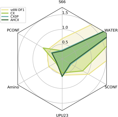
Figure 7. Performance assessment of the consistent-vdW-DF tool chain, CX-CX0P-AHCX, on 6 benchmark sets [87] of key bio-chemistry relevance, comparing relative molecule energies in: 'S66' (a balanced set), PCONF (tri- and tetra-peptide conformers), amino20X4 (amino-acid conformers), UPU23 (RNA backbone conformers), SCONF (sugar conformers), and WATER27 (binding energies of water complexes, including some cases with proton transfers). We show mean-absolute deviation (MAD) values (expressed in kcal mol−1) from quantum-chemistry CCSD(T) reference calculations [87], noting that the performance of the unscreened hybrid CX0P (turquoise curve) is almost on par with that of the RSH AHCX (dark green curve). We also include a performance overview of the original vdW-DF1 version [17] that shares the nonlocal-correlation energy formulation. Use of the consistent-vdW-DF tool chain on the WATER27 benchmarking yields larger MAD values, (around 2.85 kcal mol−1), table 4.
Download figure:
Standard image High-resolution imageTable 4 summarizes our full comparison of biomolecule performance. The top three rows quantify the figure 7 performance overview for the CX-based tool chain, reporting MAD values (in kcal mol−1) for the specific benchmark sets as well an average MAD measure (obtained by assuming equal weights among the 6 benchmark results for every functional). The table permits a quantitative comparison of CX, CX0P, and AHCX performance with benchmarking results obtained for other members of the vdW-DF family and for two dispersion-corrected functionals, revPBE + D3 [33, 85, 86] and HSE + D3 [12, 86]. The latter are closely related to the PBE-based semilocal tool chain and we note that revPBE + D3 is identified as the top performer of the Grimme-D3 corrected GGAs [87]. revPBE + D3 is a generalist that also does well for the here-considered biomolecular subset of the full GMTKN55 molecular testing suite [87]. The CX has a similar generalist status [15, 25], and table 4 shows that CX matches the revPBE + D3 performance also in this more targeted survey. Moreover, we find that the hybrid forms, CX0P and AHCX, improve the accuracy for biomolecular problems, as asserted in this test.
Table 4. Comparison of functional performance on the biomolecule-relevant subset of the GMTKN55 benchmark suite [87]. The columns identify the here-selected benchmark sets that are introduced and discussed in figure 7 and in the text. We list mean-absolute deviations (MADs) in kcal mol−1, for process energies as asserted relative to coupled-cluster calculations (at fixed coordinates) [87] for the CX-based tool chain, for other members in the vdW-DF family of nonlocal-correlation functionals (identified by citations when not previously discussed), and, lastly, for dispersion-corrected members closely related to the PBE-based tool chain. The 'Avg.' column reports an average of MAD, obtained by summing the benchmark MADs and dividing by 6. Boldface entries identify a strong performance, i.e., cases where the functional is found to have an average MAD value below 1 kcal mol−1 in this biomolecular benchmarking.
| Functional | S66 | PCONF21 | Amino20X4 | UPU23 | SCONF | WATER27 | 'Avg.' |
|---|---|---|---|---|---|---|---|
| CX | 0.283 | 0.746 | 0.254 | 0.472 | 0.808 | 2.906 | 0.911 |
| CX0P | 0.302 | 0.421 | 0.218 | 0.602 | 0.350 | 2.880 | 0.795 |
| AHCX | 0.267 | 0.400 | 0.215 | 0.585 | 0.319 | 2.841 | 0.771 |
| rVV10 | 0.428 | 0.734 | 0.332 | 0.427 | 1.077 | 11.245 | 2.374 |
| vdW-DF1 | 0.693 | 0.599 | 0.526 | 0.545 | 1.041 | 7.721 | 1.854 |
| vdW-DF-C09 | 0.383 | 0.944 | 0.346 | 0.643 | 1.386 | 8.015 | 1.953 |
| vdW-DF-optB88 | 0.361 | 0.746 | 0.227 | 0.643 | 0.754 | 5.384 | 1.353 |
| vdW-DF-optB86 | 0.346 | 0.772 | 0.245 | 0.655 | 0.871 | 5.720 | 1.435 |
| vdW-DF2 | 0.315 | 0.390 | 0.380 | 0.532 | 0.524 | 1.655 | 0.633 |
| vdW-DF2-b86r | 0.361 | 0.679 | 0.222 | 0.367 | 0.763 | 5.175 | 1.261 |
| revPBE + D3 | 0.251 | 1.009 | 0.345 | 0.598 | 0.505 | 2.579 | 0.881 |
| HSE + D3 | 0.392 | 1.337 | 0.294 | 0.704 | 0.211 | 5.881 | 1.470 |
aReferences [79, 80]. bReferences [17, 81]. cReferences [17, 82]. dReferences [17, 83]. eReferences [37, 84]. fReferences [33, 85, 86]. gReferences [12, 86].
Interestingly, table 4 identifies the vdW-DF2 as the best overall performer, primarily because of its ability to accurate describe the energies involved in the WATER27 processes. From our broader molecular surveys, summarized in references [15, 25], we find that vdW-DF2 is only a fair competitor to the CX performance on noncovalent interactions, but it is exceptionally strong in a select few benchmarks, such as WATER27. This fact deserves a separate exploration, that we generally defer. However, for the ferroelectric polymer-crystal characterization (below), we include results for both vdW-DF2 and CX, comparing also with previous theory results [147, 149].
The WATER27 benchmark set constitutes a challenge for most XC functionals [25, 87]. Even here we find that the consistent-vdW-DF tool chain delivers a robust description, with a MAD value of 2.8 kcal mol−1 for AHCX and almost as good for the nonhybrid CX form.
Overall, this survey suggests that CX and its tool chain are useful for determining interaction energies in biochemistry and, we expect, in both bio- and synthetic polymers.
6.2. DNA-intercalation energies
Additionally, we test the CX performance and robustness against recent higher-level calculational results on DNA intercalation [128]. That study identifies a set of relevant frozen (reference-coordinate) geometries, figure 6, for which it also provides coupled cluster CCSD(T) reference energies of the energy gain by molecule insertion (ignoring elastic-energy costs). We use those results for an extra test of the CX performance, because the applied DNA modeling circumvents the need for a detailed study of the effects of counter ions and water: we can directly compare our DFT results against listed reference energies at specified coordinates [128].
The basic idea is to consider two models of a DNA base-pair segment, namely one where the backbone is protonated (effectively placing one extra electron per phosphor group on the back bone structure), and one where the back-bone is further eliminated. In reference [128] the atomic positions of the three intercalants, along with those of the immediate surrounding DNA structure, were extracted from the protein database (PDB) [153]. The structures used for the CCSD(T) results were truncated to the base pairs above and below the intercalant, plus the part of the sugar-phosphate backbone that connects them (model 'B', top panel of figure 6), or without the backbone (model 'A'). The interaction energies were calculated using the focal point approach [154] for extrapolated CCSD(T) results. There are reference energies (and structures) for both models with 3 intercalants, that are all effectively nearly flat, figure 6, for the parts that are inserted in the DNA; in addition, there are also reference energies for a variant process, where the intercalant is itself protonated.
Table 5 summarizes our CX results for the energy gains by DNA intercalation for the three intercalants and in model 'A' and 'B'. The comparison is made against the CCSD(T)-extrapolated results from reference [128], and with their B3LYP-D3, and HF-3c results. The three intercalants have PDB codes 1K9G, 1DL8 and 1Z3F and are here (and in reference [128]) denoted '1', '2', and '3' (see top and middle panels of figure 6). The latter molecule includes a nitrogen atom that can be protonated and this is also included in the set of calculations, the protonated molecule is denoted '3+'.
Table 5. Comparison of CX intercalation energies, in kcal mol−1, with CCSD(T), B3LYP-D3, and HF-3c results from reference [128]. All structures are computed at the experimentally motivated reference geometries, considering two DNA models, denoted 'A' and 'B', that both have two base pairs; model 'A' and model 'B' excludes and includes a (protonated) backbone, respectively [128]. A set of CCSD(T) reference energies exist for three intercalating molecules, here labeled '1', '2', and '3', as well as for a protonated molecule variant, denoted '3+'. The comparison with dispersion-corrected B3LYP results are for results obtained with the def2-TZVP basis set, using the Becke–Johnson damping function [155] on the semi-empirical Grimme-D3 correction term [86, 87]. The MADs from the CCSD(T)-calculations are given for CX, B3LYP-D3, and HF-3c.
| System | CX | CCSD(T) | B3LYP-D3 | HF-3c |
|---|---|---|---|---|
| 1 A | −39.65 | −41.99 | −41.1 | −40.3 |
| 2 A | −39.51 | −39.52 | −39.9 | −35.7 |
| 3 A | −34.09 | −34.57 | −34.4 | −32.4 |
| 3+ A | −47.04 | −47.74 | −47.9 | −44.5 |
| 1 B | −43.60 | −45.44 | −45.2 | −44.3 |
| 2 B | −45.25 | −45.25 | −45.7 | −42.5 |
| 3 B | −39.86 | −39.39 | −40.2 | −39.1 |
| 3+B | −61.86 | −62.55 | −63.8 | −61.6 |
| MAD | 0.82 | — | 0.54 | 2.00 |
Inspecting the numbers in table 5, we see that CX yields results that are close to those from the CCSD(T) calculations, also for the protonated molecule ('3+'). This holds regardless if the DNA backbone is included (model 'B') or not (model 'A'). The largest deviation for CX is seen for molecule '1' (in both DNA models), with a 1.8–2.4 kcal mol−1 difference from the CCSD(T)-energies. All other deviations are less than 0.7 kcal mol−1, and MAD is 0.82 kcal mol−1 for CX with respect to CCSD(T). This can be compared to the B3LYP-D3 deviations from CCSD(T), that show a slightly smaller MAD (0.54 kcal mol−1) on the set of intercalate structures. However, B3LYP-D3 (and HF-3c) are hybrid calculations, and in plane-wave codes molecular hybrid calculations are found to be up to 30 times slower compared to regular functionals, like CX, for similar system sizes [15].
Turning to a comparison with results for the minimal-basis method HF-3c [128], we see that the MAD value for HF-3c, at 2.00 kcal mol−1, is more than double that for CX. In other words, CX competes well with the best hybrid results of reference [128], and offers a path to acceleration that gives improved predictability compared to the HF-3c minimal-basis-set approach.
6.3. Predicting properties of the ferroelectric PVDF polymer crystal
Finally, for our soft-matter application study, we characterize primarily the β crystalline form of the PVDF system, while also comparing with the so-called γ forms, figure 6. We predict the relaxed structure and ferroelectric response of perfect crystals of β- and γ-PVDF, while comparing with experiments and other theory results when possible. Both forms can be synthesized but, to the best of our knowledge, large single-crystal samples, with long-range order, do not yet exist. Theoretical predictions are thus motivated and we here seek to provide primarily a CX characterization in a 2 × 2 × 8 Monkhorst-Pack grid sampling of the Brillouin zone. We compute the single-chain energy Echain in a unit-cell that has twice the lateral (non-chain) extensions than what holds in the experimental characterizations.
In analogy with equation (11), we compute the polymer-crystal cohesive energy,

for a series of unit-cell lattice constants in the β-PVDF form as well as for the motifs of the γ-PVDF form. We use the stress-vdW-DF implementation in QUANTUM ESPRESSO, although we did not have to here rely on the new spin-stress extension.
Figure 8 shows an overview of the structure search and potential-energy landscape for deformations of β-PVDF that we have computed using CX (as well as in vdW-DF1 and vdW-DF2). We first establish the energy dependence of the along-chain lattice constant (using constrained variable-cell calculations) as shown in the left panel. Then, at the optimal value c0 we can extract the overall structure characterization, identified by the star shown in the right panel. In this panel, we furthermore report computed CX results for the energy variation  and a contour mapping of a fourth-order polynomial fit, tracking the energy variation in the soft interchain directions a and b [104, 139, 148].

Figure 8. PVDF energy dependence on lattice parameters generated by a set of CX calculations (dots). The (left panel) shows the cohesive energy for a constrained optimization, the (right panel) shows contours for the energy variation along unit-cell directions a and b. This contour plot is generated from a mesh of fully relaxed calculations in frozen unit cells (having structures identified by the set of dots). The energy landscapes are given relative to the energy of the optimal crystal structure (marked by the star in right panel). The black triangle and square are the relaxed results using vdW-DF and vdW-DF2, respectively [149], while the black cross shows relaxed result for PBE0 [145]. The red cross shows the results from x-ray diffraction on a sample drawn at 323 K [133] while the red square is x-ray diffraction from reference [134].
Download figure:
Standard image High-resolution image
Table 6 summarizes the CX structure characterization along with those obtained using vdW-DF1 and vdW-DF2 and those found in literature. We note that the c0-lattice constant is set by covalent interactions and that all functionals are overall in fair agreement of c0. The functional characterizations differ primarily by the predictions of the soft lattice constants a and b. It is therefore natural to use the contour plot to illustrate the functional variations on PVDF structure determinations, as also done in the (right panel) of figure 8.
Table 6. Calculated lattice parameters for the β-PVDF crystal. We compare with literature calculational results and data from room-temperature experiments.
| a0 (Å) | b0 (Å) | c0 (Å) | Ω (Å3) | |
|---|---|---|---|---|
| PBE0 | 8.64 | 4.82 | 2.64 | 109.2 |
| PBE | 8.95 | 5.00 | 2.59 | 115.7 |
| LDA | 7.97 | 4.46 | 2.56 | 90.2 |
| PBE + D2 | 8.27 | 4.55 | 2.58 | 97.0 |
| vdW-DF1 | 8.62 | 4.80 | 2.60 | 107.5 |
| vdW-DF2 | 8.40 | 4.66 | 2.60 | 101.8 |
| vdW-DF1 | 8.61 | 4.79 | 2.60 | 107.1 |
| vdW-DF2 | 8.38 | 4.67 | 2.59 | 101.5 |
| CX, constrained fit | 8.581 | 4.763 | 2.575 | 105.3 |
| CX, vc-relax | 8.585 | 4.745 | 2.575 | 104.9 |
| X-ray diffraction | 8.47 | 4.90 | 2.56 | 106.2 |
| X-ray diffraction | 8.58 | 4.91 | 2.56 | 107.8 |
aReference [145]. bReference [149]; dispersion correction 'D2' from reference [156]. cReference [133]. dReference [134].
We find that CX results obtained with the above-described constrained-fit procedure align with those obtained in a constraint-free variable-cell optimization. However, that is true only when we start the system description of the polymer crystal close to the actual ground-state structure. In table 6 we give an extra decimal in the reporting to facilitate this comparison.
We also find that CX provides a highly accurate prediction of the optimal c lattice constant for the β-form relative to experiments; that is, the description of unit-cell extension along the polymer chains is almost spot-on the experimental observation. In the other directions, we find an overestimation of the a lattice constant but an underestimation of the b lattice constant. The PBE0 and vdW-DF1 results are in closer agreement with the b lattice constant, but there the c lattice constant is significantly overestimated.
The study of the γ-PVDF crystal offers additional opportunities for a theory-experiment comparison. These crystal forms are only nearly orthorhombic, characterized by a tilt angle between the a–b basis plane and the c axis that is (as for β-PVDF) aligned with the polymer strains. The comparison is complicated by the fact that there are two conformers, denoted γu and γd , see figure 6.
Table 7 shows the results of a vdW-DF1, vdW-DF2, and CX structure characterization, along with experimental observations for γ-PVDF [157]. These reference values are obtained at room temperature in systems that are known to contain a mixture of the two motifs, i.e., both γu and γd . Thus, one would expect the volume Ω, the tilt-angle, and the lengths of the set of unit-cell vectors to be a linear combination of γu and γd values. Moreover, polymers are known to exhibits a significant temperature expansion [150]. Consequently, a good description should have a predicted volume that is smaller than the volume measured at 300 K.
Table 7. Unit-cell parameters for γ-phases of PVDF. We compare present results as well as literature values. The experimental values rely on a sample that contains a mixture of the up and down configurations, characterized at T = 300 K. The unit cell is nearly orthorhombic, with a small tilt of the along-strain axis c and the a–b basis plane.
| Functional |

|

|

|

| ∠ac(°) |
|---|---|---|---|---|---|
| γ d phase | |||||
| PBE + D2 | 9.09 | 4.96 | 9.33 | 420.2 | 89.9 |
| vdW-DF1 | 9.38 | 5.16 | 9.46 | 457.0 | 90.0 |
| vdW-DF2 | 9.12 | 5.04 | 9.45 | 434.3 | 89.8 |
| vdW-DF1 | 9.41 | 5.08 | 9.50 | 455.0 | 90.0 |
| vdW-DF2 | 9.17 | 4.99 | 9.43 | 431.9 | 90.2 |
| CX | 9.31 | 5.02 | 9.60 | 449.3 | 90.0 |
| γ u phase | |||||
| PBE + D2 | 9.38 | 4.78 | 9.24 | 414.2 | 93.3 |
| vdW-DF1 | 9.71 | 4.95 | 9.34 | 447.7 | 94.4 |
| vdW-DF2 | 9.41 | 4.85 | 9.33 | 424.8 | 94.5 |
| vdW-DF1 | 9.60 | 4.98 | 9.31 | 444.3 | 96.5 |
| vdW-DF2 | 9.34 | 4.86 | 9.31 | 421.4 | 96.0 |
| CX | 9.36 | 4.84 | 9.32 | 421.8 | 94.6 |
| Experiment | |||||
| γ u & γ d | 9.67 | 4.96 | 9.20 | 440.65 | 93 |
aReference [149]; dispersion correction 'D2' from reference [156]. bReference [157].
We find that the computed structures for the γd motif differ from the room-temperature experimental characterization, for all vdW-DF functionals. The tilt angle differs and so does the prediction for the along-chain extension (length of c). The CX characterization of the γd motif is overall not as close to the measurement as vdW-DF2. On the one hand, this is noteworthy because CX is in related systems found accurate on molecular-crystal bonding and structure, as exemplified for β-PVDF, table 6, and in references [56, 150]. On the other hand, it is not clear that the sample in the experiment contained a large component of γd motif.
Assuming instead that the structure of the polymer sample is dominated by the γu motif, the set of vdW-DF predictions are closer to the measured data. Here, CX describes a unit-cell tilt angle that is in good agreement with the measured data. Also, both vdW-DF2 and CX are now found to give a unit-cell description that is 5% smaller than the room-temperature measurements and the CX lattice constant is now in good (within 1%) agreement with the measured c-axis extension.
Overall, the CX is found accurate on structure for β-PVDF and consistent with the mixed-γ-motif measurements.
For predictions of the PVDF polarization, we follow the ideas presented by Johnsson and co-workers [147, 149] while using the QUANTUM ESPRESSO implementation of the modern theory of polarization [89–94]. That is, we use a modified cell with one PVDF chain rotated 180°, to establish nonpolar forms for both the γ and β phases and proceed with calculations that trace the effects of electron displacements in the bandstructure description of the polymer crystals [94]. For the γu/d phases, the nonpolar nature of such reference states is discussed in reference [149]; here we focus on describing the steps that are needed to accurately determine the (larger) spontaneous polarization that results in the β phase.
First, we determine the lateral position of the axis of along-chain rotation (for each of the two chains in the unit cell) by projecting the carbon atoms onto the lateral plane defined by the a and b lattice vectors. Second, we rotate one chain around its axis and confirm the nonpolar nature of the resulting reference structure [147]; specifically, we use QUANTUM ESPRESSO to compute the polarization that we find to be an integer times the so-called polarization quanta [94] (in this case e/ac) for the response along the b direction. Third, we track the evolution of the computed polarization as we incrementally rotate the chain back toward the actual PVDF β-phase structure, noting shifts among multiple branches of the polarization description in the Berry-phase formulation [89, 90, 93]. Finally, we extract the spontaneous polarization result, correcting for the impact of these polarization-branch jumps [94].
Table 8 summarises the outcome of these polarization-response surveys comparing also to previous vdW-DF1 and vdW-DF2 results [147, 149] for the γ and β phases. We note that our calculations are performed under the assumption of having a perfect crystal at the optimal structure (as computed for each of the vdW-DFs). We provide these theoretical characterizations not as a performance assessment but as an application example.
Table 8. Results for spontaneous polarisation of the three PVDF phases, studied using different vdW-DF releases and in experiments and listed in units of μC cm−2. We list present predictions as well as (in parenthesis) those obtained in previous vdW-DF1 and vdW-DF2 studies.
| Phase | vdW-DF1 | vdW-DF2 | CX | Exp. |
|---|---|---|---|---|
| β | 19.6 (19.8 | 22.5 (22.6 | 19.3 | 10 |
| γu | 7.9 (8.4 | 11.4 (6.9 | 8.3 | 0.2–0.3 |
| γd | 6.9 (10.7 | 13.3 (5.8 | 7.3 | 0.2–0.3 |
aReference [147]. bReference [135]. cReference [149]. dReference [158].
We find that CX characterizations are consistent with those provided with vdW-DF1 and vdW-DF2 for all three phases of PVDF. We also find that our vdW-DF1 and vdW-DF2 results in turn are in fair agreement (at least for the β phase) with previous theory characterizations [147, 149]. Comparison with experimental results (also listed) is difficult because of the challenges in securing fully crystalline samples, and polarization measurements will be affected by compensating responses arising in different sample regions. Nevertheless, we confirm that the β-PVDF form has the highest limit on the polarization response of the investigated phases.
In summary, we find that with a realization of a β-PVDF single crystal form, this ferroelectric polymer has a spontaneous polarization that is significantly larger than what is seen in present measurements [135]. The β phase may eventually serve as a good organic ferroelectrics.
7. Discussion and summary
An overall goal of this theory, code, validation and application paper was to illustrate potential materials-theory advantages of having a tool chain of related consistent-vdW-DF XC functionals, namely CX, CX0P, and the new AHCX. Our range-separated AHCX hybrid is very new, but we have been able to include a few examples that nevertheless identify application strengths beyond those discussed in the AHCX launching work [15]. By providing a CX-based set of related XC tools, we have the option of including both truly nonlocal correlation and truly nonlocal exchange (to an increasing extent) all within the electron-gas tradition. As such it provides the same advantages for vdW-dominated problems (and hard and soft matter in general) that the PBE-PBE0-HSE chain provides in the framework of semilocal-correlation descriptions. It provides a platform for developing a systematic analysis, as the consistent-vdW-DF application range grows.
More specific goals were to upgrade the proper spin vdW-DF formulation with a stress description and to illustrate a simple framework for understanding stability in a given DFT-based modeling. We sought the goals to facilitate modeling from hard to soft matter (inside our new XC tool chain). Here we have (1) coded the spin-vdW-DF stress result in QUANTUM ESPRESSO to enable variable-cell vdW-DF calculations in spin systems and (2) used a simple stability condition to discuss soft modes in SrTiO3, as an example. Having access to a simple, generic, stability gauge means that DFT practitioners have the option of seeking the most relevant DFT input (controlled by the XC choice) before proceeding with advanced modeling.
We have documented the spin-stress method contribution for magnetic elements as well as for a magnetic perovskite. In addition, we have also provided hard- and soft-matter illustrations by using the new tool chain of consistent-vdW-DF XC functionals on benchmarks, a new test of CX performance on DNA intercalation, and a ferroelectric-polymer application of the CX version.
Overall, we find that we will in general need more than just the CX part of the new nonlocal-correlation XC tool chain to cover materials from hard to soft. The AHCX improves the description of the magnetic Fe element over CX and both CX0P and AHCX are strong performers in our bio-relevant molecular benchmarking. However, hybrid vdW-DFs are not universally improving descriptions either, as discussed for SrTiO3. The perovskites provide examples where more studies are needed to assert when we can systematically leverage hybrid advantages in combination with truly nonlocal correlations. For the perovskites we must also explore whether to rely on the screened AHCX formulation instead of the unscreened CX0P form, at least in cases with an actual or incipient ferroelectric transition and hence significant vibrational contributions to the dielectric constant.
We present these results by looking at a number of hard and soft material cases, in the hope that they may stimulate further work and analysis. Studies using different—but closely related—regular/hybrid vdW-DFs are interesting not only because they give useful results and, overall, accurate predictions. The closeness in the XC nature of our tool chain means that variations in performance may teach us to better weigh the balance (and screening) of truly nonlocal exchange in combination with our truly-nonlocal-correlation vdW-DF framework. We therefore intend to use of the consistent-vdW-DF tool chain more broadly to continue to gather performance statistics. Ultimately we aim to learn to better identify, a priori, the best DFT tool for a given material challenge.
Acknowledgments
This paper is dedicated to Gerald D Mahan (who sadly passed away on November 22, 2021 and) whom we thank for input far beyond the ideas summarized in appendix B. We also thank Göran Wahnström for useful discussions. Work is supported by the Swedish Research Council (VR) through Grant Nos. 2014-4310, 2016-04162, 2018-03964, and 2020-04997, the Swedish Foundation for Strategic research (SSF) through Grants IMF17-0324 and SM17-0020, Sweden's Innovation Agency (Vinnova) through Project No. 2020-05179, as well as the Chalmers Area-of-Advance-Production theory activities and the Chalmers Excellence Initiative Nano. The authors also acknowledge computer allocations from the Swedish National Infrastructure for Computing (SNIC), under Contracts SNIC2019-1-12, SNIC2020-3-13, and from the Chalmers Centre for Computing, Science and Engineering (C3SE).
Data availability statement
All data that support the findings of this study are included within the article (and any supplementary files).
Appendix A.: Coordinate transformations and stress
We consider small deformations, such that the displacements can be expressed in terms of the strain tensor ɛα,β . This tensor describes coordinate transformations or scaling

Here the subscripts, α or β, identify Cartesian coordinates of the position vector
r
. We seek to express the resulting stress that arises from the spin formulation  of the nonlocal-correlation energy. This stress is formally given as a strain derivative

where V denotes the unit-cell volume.
We therefore aim to track every way that the coordinate scaling affects equation (5), for example, through the double spatial integrations, from the spin-density components ns=↑,↓( r ), and from the kernel Φ dependence on coordinate separation D. We also need to track the stress that arises because the local inverse length scale q0( r ) (inside Φ) depends on the spin-density gradients ∇ns=↑,↓( r ). These gradients change with coordinate scaling because scaling implies both a density change and a change in taking the derivative with positions. The approach is simply to apply the chain rule for derivatives with strain.
The transformation Jacobian is to lowest order

and corresponds to the strain derivative ∂J/∂ɛα,β
= δα,β
. Since  involves a double integration, this volume effect alone produces the stress contribution
  in equations (6) and (9).
The kernel Φ in equation (5) contains a term that depends explicitly on the separation D between two positions of the electron spin-density distributions. That term resembles the Hartree (or mean-field Coulomb) energy and gives a stress component defined by the second row of equations (9) and (7). Of course, for the spin-polarized case, one must evaluate the kernel derivative ∂Φ/∂D at inverse length scale values, q0( r ) and q0( r'), for the actual spin-density distributions ns=↑,↓( r ). However, that information is already available from any computations of the spin vdW-DF description of the nonlocal XC energy and XC potential.
In reciprocal space, the scaling is given by the transpose of −ɛα,β . For example, a reciprocal lattice vector scales as

It can readily be shown that with a planewave basis for wavefunctions  there are cancellations of strain effects in all but the normalization factors
  . The spin-density components ns=↑,↓ will therefore scale with derivatives given by the volume factor

However, following the logic of the original Nielsen and Martin analysis [78], the volume scaling of the densities can be summarized in terms of the relevant (spin-resolved) components  of the XC potential. The stress term
  in equations (6) and (9) summarizes all of the density-volume scaling effects for the spin-balanced and spin-polarized cases, respectively.
This finally brings us to the third row of equation (9). Here we capture the effects of strain scaling of the spin density gradient ∇ns( r ), by assuming a fixed ns( r ) variation:

For the length of this derivatives we have

because we have handled the volume scaling of the density separately [78]. The third row of the spin-vdW-DF stress description equation (9) follows by a simple application of the chain rule.
Appendix B.: Navigating phase transformations
Hard and soft matter come in different crystal forms, as well as meta-stable variants, and there is often a need for a concerted theory-experiment analysis to resolve and understand phase stability. This is true, for example, even in simpler (compact-unit-cell and nonmagnetic) perovskites [52–55, 90, 111–113, 115, 159–171] and in both nonpolar and ferroelectric polymers [100, 132–136, 140, 144–149, 158]. The structural transformations may be driven by temperature, electric fields, or strain; there can also be a release from meta-stable states that may have been locked in under synthesis or by usage [100].
Effective modeling beyond DFT calculations of structure and modes is important. First-principle calculations may help in the analysis with volume-constrained variable-cell calculations and by determination of the phonon spectra, as well as calculations of magnetic, elastic, polarization, and strain response [89, 90, 100, 115, 116, 125, 140, 144, 146, 147, 149, 171–179]. For a given XC functional, we can rely on the BO approximation to determine what we call the native structure. We can also compute the phonon spectra at the native structure or at the experimental structure and, for example, check for soft modes [54, 55]. However, finding of an imaginary frequency in a BO description simply says that there is an incipient instability for the chosen XC functional. We must track zero-temperature and thermal fluctuations to assert if that XC functional predicts an actual phase transformation [112, 115, 171] or facilitates a polymer breakdown of long-range phase order [100]. For the compact-structure perovskites (like SrTiO3), there exists both Monte-Carlo simulation frameworks [112, 113, 166, 167] and a phonon Green function formulation [115, 125, 171]. However, something simpler is, in general, desirable to limit the computational load in complex systems.
Here, we illustrate the use of a model analysis of quantum effects on transformations. The approach is generic to stability problems. Our model is inspired by a quantum theory of fluctuations above the phase-transition temperature [43] but it also takes tunneling-induced vibrational-mode-level splitting into account. We focus the discussion on the SrTiO3 AFD mode, and compare DFT characterizations obtained for a string of XC functionals.
The important step is to set up a size-consistent description of the vibrational mode that may drive distortions. The Hamiltonian for the ionic motion in generalised canonical coordinates (denoted Qs q ), can be written

The band index is s, and q denotes the phonon momentum. The set of Qs
q
's reflect the atomic displacements  and the phonon eigenvector
  through the relation

where η denotes the Cartesian coordinate. Here  is the number of assumed Born-von Karman repetitions, while Rn
and Mn
denote the position and mass of the n'th atom in the unit cell. For studying the stability of the AFD mode in the cubic structure only the phonon wavevector at the R point is needed. Also, as illustrated in figure 3, the AFD modes exclusively express oxygen rotations, leaving only oxygen-related terms in (B2). Thus we can set Mn
= M ≡ 15.999 atomic mass units (which we denote u).
is the number of assumed Born-von Karman repetitions, while Rn
and Mn
denote the position and mass of the n'th atom in the unit cell. For studying the stability of the AFD mode in the cubic structure only the phonon wavevector at the R point is needed. Also, as illustrated in figure 3, the AFD modes exclusively express oxygen rotations, leaving only oxygen-related terms in (B2). Thus we can set Mn
= M ≡ 15.999 atomic mass units (which we denote u).
For a non-interacting single-R-phonon mode, the potential energy variation can be approximated to the fourth order in the AFD displacement d, or equivalently in the canonical coordinate in the specific mode, Q [44]. The resulting Landau expansion is

Here,  and
and  are effective material-specific constants of the Landau expansion for the AFD mode, reflecting both the effective interatomic couplings and inertia of the atoms involved in the dynamics [44]. The overbar is used to distinguish these parameters from those characterizing a (related) expansion of the PES expressed in terms of AFD-type distortions (here denoted d) [54, 55], rather than phonon-mode coordinate Q.
The potential energy in equation (B3) scales properly with respect to the chosen size of the supercell or Born–von Karman representation, i.e., with  . A doubling of the simulation cell in every direction (
 ) yields the coordinate rescaling,
  , and the potential-energy rescaling

Size consistency also holds for the kinetic-energy part and for the set of vibrational frequencies ωi
that emerge as solutions to the eigenvalue problem defined by the Landau-expansion Hamiltonian, equation (B3). These frequencies characterize the model dynamics and will, in principle, reflect tunneling when  .
.
For our parameter fittings, we note that figure 5 shows the total-energy variation (in a single cell of 40 atoms) as a function of the scaled AFD mode coordinate Q. The AFD mode in SrTiO3 exclusively involves 16 identical oxygen and the same values define the magnitudes of the relevant oxygen displacements d and the relevant eigenvector components, denoted v. Normalization mandates that v2 = 1/16 and, in this simplified description, equation (B2) formally reduces to  . We use
  for defining the coordinate scaling Q, as we fit
  and
and  to the 40-atom PES shown in figure 5. The relation among quadratic coefficients (κ and
  ) in the related PES expansions,
  , is
, is  .
.
The computed value of the coefficient  in the Landau expansion identifies the presence of an incipient instability for cubic SrTiO3 (the configuration described by Q = 0) in all of the LDA, PBE, CX, HSE, and CX0P functionals. However, we must also consider the fourth-order term. The double-well shapes produce instead vibrational-mode eigenvalues ωi
with a splitting, denoted 2Δ. The splitting is inversely related to the depth of the double well: it is very small for LDA, fairly large for CX0P and large for HSE. However, a negative
in the Landau expansion identifies the presence of an incipient instability for cubic SrTiO3 (the configuration described by Q = 0) in all of the LDA, PBE, CX, HSE, and CX0P functionals. However, we must also consider the fourth-order term. The double-well shapes produce instead vibrational-mode eigenvalues ωi
with a splitting, denoted 2Δ. The splitting is inversely related to the depth of the double well: it is very small for LDA, fairly large for CX0P and large for HSE. However, a negative  value does not necessarily imply a prediction of an actual deformation. Instead the question of stability comes down to a competition between the speed of the inter-well tunneling and the rate of which we can expect dephasing, as further discussed in section 5.2.
We motivate the stability condition, equation (13) of section 5.2, as follows: tunneling, as well as thermally activated fluctuations, will connect the dynamics in both wells. The tunneling might be so slow that dephasing scattering occurs, preventing the mode from maintaining the coherence that exists in an isolated quantum-mechanical double-well problem. In that case the inter-well dynamics is instead exclusively caused by thermal activation and there will (at T = 0) be a lock-in into one of the wells. We interpret this lock-in as corresponding to an actual low-temperature transformation as T → 0, and such transformation occurs in an LDA description of SrTiO3 and BaZrO3. It will also happen in CX, but it is not a result that emerges in our CX0P study of SrTiO3, section 5.2.
The overall idea is perhaps best illustrated by an analogy to first-principle-theory-based analysis of addimer diffusion on metals, a problem that also provides a measured estimate for τscat ∼ 1 ps [180]. In the adatom/addimer-diffusion problems, for example, explored in references [181–187], the dynamics eventually rolls over to a tunneling regime [183]. A scanning-tunneling microscopy study documents that the addimer dynamics will never freeze out [180]. The roll over to quantum-tunneling transport occurs below Tcross = 5 K, corresponding to kB Tcross ≈ 1 meV. This energy scale sets the time scale for τscat = ℏ/kB Tcross ≈ 0.7 ps. The low-temperature dynamics of Cu(111) addimers cannot be seen as thermally activated hopping. Rather, the dynamics maintains phase coherence and no actual lock in or trapping occurs [180, 183].