

Abstract
The spectral emissions from a microplasma have been used to predict the CO2 concentration in gas samples covering a concentration range of 0%–100%. Different models based on partial least squares have been evaluated, comparing two different spectral pre-processing filters –multiplicative scatter correction (MSC) and standard normal variate correction (SNV) – and three different wavelength ranges. The models were compared with respect to accuracy, precision, stability and linearity. CO2 samples were mixed with either air or nitrogen. The choice of mixing gas influenced the predicted concentration and basing the models on data from only one mixing gas resulted in higher prediction power. Using air as mixing gas and SNV filtering resulted in a root mean square error of prediction (RMSEP) of 0.03 for an independent test dataset. This RMSEP was of the same range as the experimental error. On the other hand, the models with the best long term stability, reaching the lowest Allan variance, were based on observations with both mixing gases. Models based on MSC filtering generally had slightly higher RMSEP than those based on SNV filtering. Generally, the CO2 concentration could be accurately predicted in the concentration range of 5%–90%. For higher and lower concentrations, the models underestimated the CO2 concentration and were less accurate and precise. Basing the models on fewer wavelengths resulted in reduced linearity. The models were also evaluated by applying them for transcutaneous blood gas monitoring, where they helped to reveal new physiological information.
Export citation and abstract BibTeX RIS
1. Introduction
The key to creating a useful gas sensor is generally to find manners of combining obvious properties like sensitivity and limit-of-detection with less obvious ones like specificity and selectivity, preferably in an easy and inexpensive way. In reality, this is very difficult since simple and cheap sensors, like those based on electrochemical [1] or semiconductor [2] principles, often lack selectivity, while highly selective or even specific sensors, like those based on laser absorption methods [3], often are very complex and expensive. One of the major reasons why high selectivity is difficult to achieve is that most sensing methods lies in the intersection between physics and chemistry where fully explanatory theoretical models of the underlying processes are next to impossible to construct. This is particularly true for plasma-based sensors since the properties of any plasma is dependent on a multitude of physical and chemical parameters.
We have previously reported a microplasma based system for optical emission spectroscopy of CO2 [4]. This system utilizes both the physics and the chemistry of the plasma, where CO2 first is converted to CO in a chemical process, after which optical emissions from the CO Ångström system are recorded by a spectrometer. From these data, the original concentration of CO2 can be calculated. Even though the emission process is very specific, the conversion process is not, and may vary depending on the composition of the sample. For example, the conversion process was shown to be significantly influenced by the presence of O2 [4].
Moreover, the emission process is only specific in theory, but when the emissions are recorded by a spectrometer with, e.g, limited wavelength resolution, they tend to get tainted by background from closely lying peaks. Finally, the plasma itself is dependent on, e.g., the supplied power and process pressure, and variations in these ambient properties affect it greatly. All of these effects make the measurement sensitive to variations in the concentration of other species in the sample, and, hence, reduces the specificity.
However, the recorded spectrum consists of data from UV to near-IR wavelengths and contains information of all species, not only CO2 and CO. Still, only about 1.5% of this data was used to calculate the CO2 concentration [4]. Hence, by using more, or even all, of the spectrum to try to compensate for the background in the signal, it should be possible to improve not only the specificity but also the precision, accuracy and stability of the measurement.
In this paper, we create analytical models of the plasma emissions based on partial least square (PLS) regression analysis to predict the CO2 concentration and identify the variables that co-vary with it.
Finally, to paraphrase Helmut von Moltke the Elder, models rarely survive the first contact with reality. Hence, to truly evaluate the performance of the models, they were tested in a real application where the microplasma emission spectrometer was used as a transcutaneous blood gas monitor (TBM). In this method, the concentration of dissolved CO2 in blood and tissue is measured by collecting and analysing the minute amounts of gas that permeates the skin [5]. The employed TBM setup is thoroughly described in [6]. Using these and other measurements on samples with known CO2 concentration, the precision, accuracy and stability of the modelled responses were calculated and compared, both to each other and to the previously reported analytical method.
2. Materials and method
2.1. Measurements
The microplasma source used in this study was a stripline split-ring resonator (SSRR) [7] with a 2 mm wide gap. It was fabricated from two RO4003C (Rogers Corporation, AZ, USA) printed circuit boards with 35 μm thick Cu cladding. The resonance frequency of the ring was 2.497 GHz. The SSRR was mounted inside a commercial microplasma emission spectrometer (Pithos, Fourth State Systems AB, Sweden) with a custom-made RF power supply that was connected to the SSRR with UltraMiniature Connectors. The gap via of the SSRR was connected to a fluidic system that continuously flowed gas through the plasma at a rate of about 0.1 μmole/s, which resulted in a process pressure of 90–100 Pa. The light emitted from the plasma was analyzed with an internal CCS200 (Thorlabs, NJ, USA) with a bandwidth of 200–1000 nm, an FWHM of 2 nm at 633 nm, a 20 μm by 2 mm slit, and a 600 lines/mm and 800 nm blaze grating. Apart from recording the emitted spectrum, process pressure, transmitted and reflected powers to the SSRR, and plasma potential.
During an experiment, gas with a fixed mixture of CO2 in either air or N2 was analyzed, while keeping other process parameters like power or pressure constant. An experiment produced a series of observations, where one observation was one emission spectrum with corresponding process parameters. Together, a set of experiments – with similar or different gas mixtures, powers, etc – formed a dataset, and one or more datasets were used to build and evaluate the models. If nothing else is specified, the plasma source was turned on one hour before the experiments to allow for thermal stabilization.
The foundation of the data used to train and validate the models was the experiments presented in [4] since the major aim of this study was to investigate if, and in that case, how, PLS regression could be used to improve the result beyond the relatively simple analytical model used there. This data set, from hereon referred to as dataset A, consisted of experiments on mixtures with 21 different gas compositions – 11 mixtures of CO2 and N2 where the CO2 concentration was varied between 0% and 100% in steps of 10%, and 10 mixtures of CO2 and air where the CO2 concentration was varied between 0% and 90% with the same step, table 1. An additional series of 11 mixtures with N2 formed dataset B. Then, to form a training set that included more system variation, certain parts of the setup from [4] were replaced, e.g., the plasma source, parts of the optics, and the vacuum pump. This remodelled version of the setup was used to create data set C, with the same gas mixtures as dataset A, but different power levels, table 1.
Table 1. Properties of the datasets for modelling, validation, testing and evaluation.
| Gas mixtures with: | Observations in: | |||||||
|---|---|---|---|---|---|---|---|---|
| Dataset | Setup | Power (dBm) | N2 | Air | Training | Validation | Test | Total |
| A | Same as [4] | 35–37 | 11 mixtures, 0%–100% CO2 in steps of 10% | 10 mixtures, 0%–90% CO2 in steps of 10% | 490 | 140 | — | 630 |
| B | Same as [4] | 35–37 | 11 mixtures, 0%–100% CO2 in steps of 10% | — | 239 | 91 | — | 330 |
| C | Remodelled | 26–33 | 11 mixtures, 0%–100% CO2 in steps of 10% | 10 mixtures, 0%–90% CO2 in steps of 10% | 622 | 218 | — | 840 |
| D | Remodelled | 27 | 10 mixtures, 5%–95%, steps of 10%, and 0 and 100% CO2 | 10 mixtures, 5%–95%, steps of 10%, and 0% CO2 | — | — | 520 | 520 |
| E | Remodelled | 30 | — | 20% CO2 | — | — | — | 3350 |
| F | Remodelled | 30 | — | Transcutaneous measurement | — | — | — | 701 |
| G | Remodelled | 27 | — | Transcutaneous measurement | — | — | — | 699 |
| H | Remodelled | 30 | — | Transcutaneous measurement | — | — | — | 700 |
To build the models, 75% of the observations in datasets A, B and C were randomly allocated to a training dataset, and the remaining 25% formed a validation dataset.
To further test the models, a fourth dataset, D, was created, consisting of experiments on CO2 mixtures with both N2 and air, with concentrations between 5% and 95% in steps of 10%. In addition to these 20 mixtures, the dataset contained another three experiments on pure samples (CO2, N2 and air).
Moreover, a fifth dataset, E, was designed to evaluate stability. Here, the output of the spectrometer was recorded directly from plasma ignition and continuously for 2 h, with a sample of 20% CO2 mixed with air. The method of mixing the samples in datasets A-E is described in detail in [4].
Finally, to enable evaluation of the models' performance in an actual application, a set of three evaluatory experiments were performed, each forming an individual dataset, F-H. These were recorded using the TBM setup. This setup consisted of two integral parts, a microplasma emission spectrometer (Pithos, Fourth State Systems AB, Sweden) that contained the plasma source, and a gas collector that was used to collect and conduct gas from the skin interface to the spectrometer. The collector consisted of a polydimethysiloxane patch with four 9.2 mm long microchannels, 400 μm in diameter, that collected gas from the surface of the skin and conducted it to the spectrometer through a 190 mm long capillary, 40 μm in diameter. The collector is described in detail in [6].
The three experiments followed the same sequence where the gas collector was successively attached to (1) The arm just below the bend of the arm, near the elbow, (2) The back of the hand between the thumb and the index finger, and (3) The tip of the thumb, all on one of the authors. The collector was attached to each site for 2 min, and then allowed to rest in ambient air for 2 min before being attached to the next site. The attachment sequence was repeated three times in an experiment, and the experiments were conducted on different days. To challenge the models, the experiments were conducted at different powers, table 1.
2.2. Modelling
The models were developed using the software Simca 16.0.2 (Sartorius Stedim Data Analytics AB, Sweden). Their performance was then analyzed and compared with Matlab (R2020a, MathWorks, MA, USA).
2.2.1. Pre-processing
At low CO2 concentration, the intensities of the resulting CO peaks were relatively low, and high plasma powers were required to get a sufficient signal-to-noise ratio. However, this simultaneously saturated some of the much stronger N2 peaks. Values corresponding to saturation in the dataset were removed, and if the total amount of data for a specific wavelength was less than 50%, the wavelength was not included in the models. Using this method wavelengths between 360.6–361.4 nm and 383.7–384.1 nm, i.e., the parts of the spectrum with the most saturation were excluded. To further study the effects of saturated spectral peaks, two more comprehensive ranges of excluded wavelengths were investigated. These are from here on referred to as reduced wavelength ranges (RWRs) 1 and 2. In RWR1, wavelengths between 339.1–438.7, 647.9–683.7, 738.4–782.4, and 889.7–895.9 nm were excluded, and in RWR2, wavelengths between 338.9–461.2 nm, 577.3–611.9 nm, 633.1–695.2 nm, 726.8–787.8 nm, and 869.3–898.7 nm were removed.
To normalize the spectra and correct for baseline shifts, two different filtering techniques were evaluated, Multiplicative Scatter Correction (MSC) and Standard Normal Variate Correction (SNV). In MSC, each spectrum Xi is regressed against the mean spectrum of all observations, Xm, to find the least squares  The corrected spectrum is then calculated as
  In SNV, each spectrum Xi is mean centred by subtracting the mean
  Then each centred spectrum is divided by its standard deviation
  giving
  [8].
[8].
2.2.2. Modelling strategies
Since one observation consists of 3647 spectral variables and 5 process parameters, any possible effect that the process parameters may have on the models are at risk of being overshadowed by effects from the great number of spectral variables. Hence, a hierarchical approach was initially evaluated and Principal Component Analysis (PCA) was used to describe the spectral variables. Then, the principal components from the PCA were used together with univariate scaled process parameters to model the CO2 concentration. This approach was compared with models built on only the spectral data.
Furthermore, PLS models based only on experiments where the same mixing gas, i.e, either N2 or air, was used were also investigated.
2.3. Model evaluation
The models were primarily evaluated and compared based on their root mean square error of prediction (RMSEP) and linearity. The latter was estimated from the R2 of a linear fit to the modelled data over the full concentration range (0%–100% CO2). In further testing, the precision, accuracy and stability of the models were also investigated. Here, the precision was determined experiment-wise as the root mean square deviation of the predicted concentration,  from the average for the experiment,
  i.e.,
i.e., ![$\left[\displaystyle \sum \left({y}_{p}-\overline{{y}_{p}}\right){}^{2}/N\right]{}^{1/2}.$](https://content.cld.iop.org/journals/2516-1067/2/4/045006/revision3/prexabd294ieqn8.gif) The accuracy was determined as the absolute difference of said average from the observed CO2 concentration,
The accuracy was determined as the absolute difference of said average from the observed CO2 concentration,  i.e.,
i.e.,  Here, the uncertainty in the mixing process had to be taken into consideration. This uncertainty depended mainly on the number of mixing steps, n, and was estimated to
  based on reference measurements using a residual gas analyzer [4]. Here, n was either 0 or 2 for pure and mixed gases, respectively. The uncertainty of the mixing process effectively sets a lower limit to the achievable accuracy and RMSEP of the models.
Finally, the stability of the modelled signal was determined as the global minimum of the Allan variance for dataset E. This minimum corresponds to the time over which the accuracy can be improved by averaging. Beyond this point, different drift processes like low-frequency noise will start to dominate the measurement.
3. Results
3.1. Hierarchical model
The first component from the PCA using MSC filtering explained 83% of the variation of the spectral data in the training set, and with 8 significant components, 98.5% could be explained. The hierarchical PLS model had one significant component explaining 97% of the variation in the CO2 concentration. The RMSEP of the validation and test sets were 0.07 and 0.06, respectively. Samples that had been mixed with air tended to be predicted with higher CO2 concentrations compared to samples of the same CO2 concentration mixed with N2. The primary influence on the model came from the first two spectral components from the PCA, where the importance of the first component was 11 times higher than the importance of the second.
3.2. Models using all wavelengths in the spectrum
Since the importance of the non-spectral variables was very low, and adding them did not increase the amount of variation explained by the model, only spectral data were used for further modelling. In addition, PCA was no longer performed before the PLS modelling.
Figure 1 shows the predicted and observed CO2 concentration when using the SNV filter. Blue squares indicate that N2 has been used as mixing gas, and red squares indicate mixing with air. The corresponding RMSEP of the validation and test sets were both 0.04.

Figure 1. Prediction of CO2 for dataset D using SNV filtering. Blue squares are mixed with N2, red squares are mixed with air and yellow are pure CO2. Observations in a single experiment overlap. The error bars indicate the uncertainty in the CO2 concentration coming from the mixing procedure.
Download figure:
Standard image High-resolution imageThe first principal component explained 96% of the variation, and the loading vector of this component revealed that wavelengths corresponding to CO and N2 peaks had strong influence on the CO2 concentration, and that several spectral peaks overlap, figure 2.
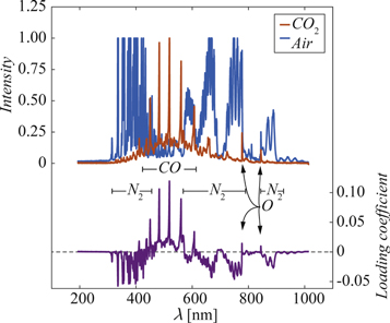
Figure 2. Typical spectrum of pure CO2 (red) and air (blue) together with the loading plot (purple) for the first principal component of the model based on SNV filtering of all wavelengths.
Download figure:
Standard image High-resolution imageThe model underestimated the CO2 concentration when N2 was used as mixing gas and, instead, overestimated the concentration when air was used. This separation was also observed for the MSC filter.
Because of this, models based on only one mixing gas were also evaluated. This improved the prediction power, e.g., reduced the RMSEP to 0.03 for the test dataset when the SNV filter was used. The best model was based on mixing with air and had linearity of 0.9973. Still, the CO2 concentration was underestimated for the lowest and highest concentrations as seen in the residual plot, figure 3. Furthermore, the precision was worst for 0% CO2, and generally, the performance of the models was reduced when the CO2 concentration was below 5%. The same general trends were observed when the MSC filter was used, though in most cases, the RMSEP was slightly higher compared to the SNV filter, figure 4.
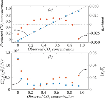
Figure 3. Residuals from predictions when the model based on SNV filtering of all wavelengths, but built on mixtures with air only, is used for predictions of the test data set (top right) and the corresponding precision (bottom left) and accuracy (bottom right) according to definitions in section 2.3.
Download figure:
Standard image High-resolution image
Figure 4. RMSEP of the models. The colours decode the filtering and the data set used.
Download figure:
Standard image High-resolution image3.3. Models using reduced wavelength ranges
Models based on reduced wavelength ranges were evaluated to investigate if the models could be improved if wavelengths corresponding to potential saturation of the bright N2 peaks were excluded. However, as more spectral information was removed from the models, the RMSEP had a strong tendency to increase, figure 4, especially for the lowest and highest CO2 concentrations. The same effect was seen in the linearity, where R2 was generally lower for RWR2, figure 5. Furthermore, the models based on RWR1 or RWR2 with both mixing gases showed the same overestimation of the CO2 concentration for mixtures with air compared to mixtures with N2 as observed before.
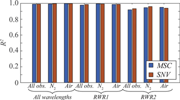
Figure 5. The linearity of the models. The colours decode the filtering used.
Download figure:
Standard image High-resolution image3.4. Test experiments
For all models, the Allan variance was calculated based on either all observations in data set E, or for observations from the last hour only, where the system had stabilized thermally, figure 6(a). The former variance was consistently higher than the latter, indicating that the models could not fully predict the additional variations during the thermal stabilization. Given that air was used as mixing gas in data set E, models based on N2 as mixing gas was not analyzed. The most stable models, reaching the lowest Allan variance, were based on observations with both mixing gases. Here, the SNV and MSC filters were about as effective in creating stable models. For MSC, when employing RWR1, the stability was moderately affected, but with RWR2 it was significantly reduced. For SNV, the best stability was obtained for RWR1.

Figure 6. Box plots showing the minimum Allan variance (a), precision (b) and accuracy (c), as defined in section 2.3, for all the investigated models. The the minimum Allan variance was calculated either for all of dataset E, or for its last hour. The bottom two panels are based either on all the 23 experiments of dataset D, or only the 11 on mixtures with air. The dashed line in (c) corresponds to the average uncertainty in the mixing process.
Download figure:
Standard image High-resolution imageHere, it should be mentioned that the method described in [4] used much fewer wavelengths than included in RWR2, but still showed better stability than many of the models built on this wavelength range.
Regarding accuracy and precision, figures 6(b), (c) shows that the modelling strategy presented here improved both. In general, the precision was improved more than the accuracy compared to [4].
3.5. Evaluatory experiments
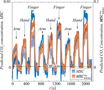
Figure 7 shows the three TBM measurements, datasets F-H, evaluated by the method in [4] and the three models that produced the most visible transcutaneous CO2 signal. This was defined as an increased CO2 concentration when the gas collector was put on the skin and a reduced concentration when it was removed. The maximum CO2 concentration expected in these experiments was in the order of 1%, i.e., in the region where the precision and accuracy of the models were lowest.
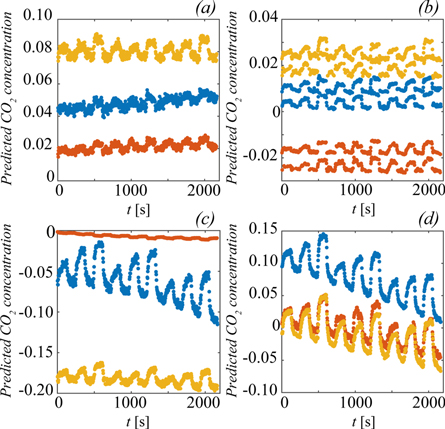
Figure 7. Analysis of datasets F-H with the method in [4] (a), and the MSC (b),  (c), and
  (d) models. The colours blue, red and yellow correspond to dataset F, G and H, respectively.
Download figure:
Standard image High-resolution imageThe three models were the MSC filtered model based on all wavelengths and all gas mixtures, the MSC filtered model based on RWR2 and only air mixtures, and the SNV filtered model based on RWR1 and only air mixtures. The other models produced more ambiguous results that were difficult to evaluate, and many showed few traces of transcutaneous signal at all.
None of the selected models gave any considerable improvement of the accuracy, here represented by the difference in base levels between the different experiments, which is not surprising since the models showed the lowest accuracy at low CO2 concentrations.
The model based on all wavelengths, figure 7(b), showed results that split into two discrete levels. Disregarding the split, the model improved both stability and precision compared to the method of [4], here visible as reduced drift in the base level and improved signal-to-noise ratio, respectively. Reducing the wavelength range to RWR2, figure 7(d), removed the split and preserved the precision improvement, but the stability started to deteriorate, as seen from the increased drift in the base level.
The SNV filtered model, figure 7(c), produced similar but more inconsistent results compared to the models based on MSC. Again, the precision was improved compared to [4], while the stability and accuracy were comparable. However, the amplitude of the transcutaneous signal varied greatly between datasets F-H. This effect was not seen for the other models.
4. Discussion
The spectral data explained most of the variation in the datasets, and as the hierarchical model showed, adding other process parameters from the plasma source (power, pressure, etc) did not improve the models. This is explained by the fact that these parameters are already expressed in the spectra where the width of the peaks relate to pressure through Lorentzian broadening, and the intensity of the peaks to the power.
Spectral peaks from the most prominent species in the plasmas – CO2, CO, N2, O2 and O – are often close and even overlapping. The approach of using a much larger part of the spectrum resulted in more reliable models with better prediction power, linearity, accuracy and precision compared to what was presented in [4], figures 4 and 6. There was a clear relationship between the obtained precision and the number of wavelengths included in the models, Nλ , i.e., the number of data points in an observation, figure 8. This indicates that much of the spectrum contains useful information, where the maximum theoretical improvement of the precision would scale with √Nλ .

Figure 8. Relationship between the achieved precision and the number of wavelengths included in the models.
Download figure:
Standard image High-resolution imageThe experimental variation in CO2 concentration coming from the mixing processes was estimated to ±0.02–0.03, i.e., comparable to the RMSEP of 0.03 that was achieved when the models were based on only one of the mixing gases. This shows that the models captured practically all systematic variation in the datasets. To improve further, more accurate gas mixtures are needed, especially when it comes to predicting CO2 concentrations below 5%. At such low concentrations, the investigated COpeaks are both drowned in background and closer to the detection limit of the spectrometer. This makes them susceptible to both wavelength drift and noise. A natural strategy to improve performance below 5% CO2 would be to increase the intensity of the recorded spectrum by either increasing the integration time of the spectrometer or the power to the plasma. However, increasing the intensity in one part of the spectrum will unconditionally lead to saturation in another, and consequently to the loss of information. One way of circumventing this would be to record two sequential observations, one with a short integration time giving little saturation, and one with long integration time giving good resolution at weaker peaks. The data of the two can then be combined to a single observation having good resolution without saturation. Another option would be to use a spectrometer with a lower detection limit. Finally, the results in figure 8 also indicates that a spectrometer with higher wavelength resolution would improve the prediction power.
The best models were based on including only observations where the same mixing gas was used. When observations with both mixing gases were included, the CO2 concentration was overestimated in air and underestimated in N2 mixtures. One probable reason for this is the complex chemistry and physics of the plasma. For example, the addition of extra O2 will affect the dissociation process of CO2 to CO, and, hence, the intensity of the most important peaks in the plasma. Such an effect was observed by us in [4] and by others in [9], but the fact that the former's method for calculating the CO2 concentration did not result in any difference between the mixing gases suggest that the reason is more complex.
Figure 9 shows the relationship between the intensities in two spectra with 90% CO2, mixed with either air or N2. The three visible linear trends suggest that there are at least three different processes active in the plasmas and that the activity of each process differs depending on the mixing gas. Furthermore, the inset shows that the processes appear to dominate different parts of the spectrum. Such a complex situation may be difficult for the models to handle and may contribute to the mixing dependent separation of the predictions. The fact that the method in [4], which did not show a split for different mixing gases, only used wavelengths in the blue part of the spectrum in the inset of figure 9, could suggest that further studies of RWRs could help to mitigate the models' dependency on mixing gas.
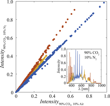
Figure 9. Relationship between the intensity of the spectrum from 90% CO2 mixed with air (x-axis) and N2 (y-axis). Each point corresponds to the intensity of a single wavelength in both spectra. The three visible linear trends, corresponding to three different plasma processes, have been colour-coded in blue, red and yellow. The inset shows the spectrum of the mix with N2 using the same colour code, hence, visualizes in which parts of the spectrum the three processes were active.
Download figure:
Standard image High-resolution imageAs figures 1 and 3 show, the performance of the models deteriorated at both low (<5%) and high (>90%) CO2 concentrations, giving the relation between the observed and predicted concentration a slight S-shape. When fewer wavelengths were included in the model, this S-shape became more pronounced, as reflected by a loss of linearity, figure 5. If different plasma processes dominate in different concentration regimes, it would, in the future, be useful to use different models for different concentration ranges.
The SNV filtered models had slightly better precision and accuracy than their MSC filtered counterparts, figure 6. Concerning stability, it was difficult to make any clear distinctions between the two filters, maybe except that the MSC filter performed best when using all wavelengths in the spectrum, while SNV prefered RWR1. However, the differences are small. It could also be mentioned that none of the filters could account for the, predominantly thermal, variations that occurred shortly after plasma ignition, as seen by the stability improvement when only the last hour of dataset E was studied. Summarizing, the difference between the two filters was small but if a distinction should be made, SNV filtering would be recommended for CO2 concentrations between 5% and 95%, given its slightly better RMSEP, precision and accuracy.s
As already discussed, the performance of the models in this paper was worst for the lowest and highest concentrations, and the performance in the TBM application is expected to improve if models developed only for the lower concentration range (0%–5%) would be used. Despite this, it is possible to make some interesting observations applying the models to the three transcutaneous experiments.
The model based on all wavelengths, figure 7(b), showed results split into two discrete levels, with a constant difference of ∼0.0069 between the two levels. The reason for this behaviour is not fully understood, but one theory is that it is caused by the way the PLS algorithm is handling saturated peaks, where there are missing values after the pre-processing. One cause of the discrete nature of the split could be that one or several wavelengths randomly jump to and from saturation. The fact that no such split was observed for the models based on the reduced datasets (RWR1 and RWR2) further strengthens this assumption. Disregarding the split, the model in figure 7(b) improved both stability and precision compared to the method of [4].
Both MSC filtered models, figures 7(b) and (d), produced curves at different base levels in the three measurements. The amplitude of the transcutaneous CO2 signal, i.e., the change in signal when the gas collector was on and off the skin, was more repeatable. Figure 10 shows the same data as in figures 7(b) and (d) after (1) Removing the shift by adding the constant 0.0069 to all points in the lower level of figure 7(b), and (2) Removing the base level in all measurements by subtracting a linear fit, fitted to the part of each measurement where the gas collector was off the skin. This revealed a situation where the transcutaneous CO2 level consistently was the lowest for the arm and the highest for the finger. The explanation for this relationship is likely physiological and depends on factors like blood perfusion and distribution, local metabolism, tissue temperature and skin thickness. Although signs of such a relationship are hinted in figure 7(a) using the method from [4], the models in this paper make it much more evident, particularly thanks to the improved precision.
Figure 10. Post-processed results of the evaluatory experiments where the base level of the curves in figures 7(b) and (d) has been removed by subtracting a linear fit, fitted to the part of each measurement where the gas collector was off the skin. The shift in figure 7(b) was also removed by adding 0.0069 to all points at the lower level of each measurement.
Download figure:
Standard image High-resolution image
Even though the transcutaneous experiments were done in the concentration region where the models show the lowest precision and accuracy, the precision of some of them were high enough to make new physiological information visible. Hence, the models have already proven to be valuable in the actual application of TBM. Creating a modelling strategy dedicated to the TBM case will be the next step. Here, stable models with improved accuracy are needed and this could likely be achieved by using a training data set that contains measurements on lower CO2 concentrations (0%–5%) only, perhaps also using a spectrometer with higher wavelength resolution or recording spectra pairwise as described above.
5. Conclusion
Using PLS modelling to predict the CO2 concentration from microplasma spectral emissions, an RMSEP of 0.03 was obtained, which was comparable with the experimental errors of ±0.02–0.03. SNV filtering resulted in models having slightly better predictive power compared to MSC filtering, and is recommended for applications with expected CO2 concentrations between 5 and 90%. Adding process parameters such as plasma power and pressure did not improve the models. At least three different chemical processes were important for the formation of CO in the plasma, and the relation between them was affected by the presence of O2. The most accurate results were obtained when only experiments with one mixing gas were included in the model, but the stability of the models was slightly better if experiments with both gases were used. If fewer wavelengths were included in the model, the prediction power was reduced and the model became less linear. When the models are used in the low concentration range, as exemplified by the transcutaneous measurements, spectrometer saturation at some wavelengths affects particularly the accuracy. To extend the improvements that the PLS modelling strategy offers to the TBM application, it is necessary to add more training data at low CO2 concentrations and make dedicated models in this regime.
Acknowledgments
This project has received funding from FORMAS (No. 2016-00706) and ATTRACT, funded by the EC under Grant Agreement 777222. The Knut and Alice Wallenberg Foundation is acknowledged for funding the cleanroom facilities. The authors would also like to acknowledge Martin Berglund at Fourth State Systems AB for help with both hardware and software issues, and Ragnar Seton att Uppsala University for help with the gas collector.
Conflict of interest
Anders Persson is a partner of Fourth State Systems AB that produces the spectrometer system used in this study.