
Abstract
Using a magnetic mirror plasma device, helium ion temperatures were investigated using high resolution Doppler spectroscopy of the He II line at 468.6 nm. The objective was to improve the quality of fits to Langmuir probe data. Measured temperatures, which represent an average value over a line of sight, ranged from 0.07 eV to 0.32 eV with higher values reached in stronger magnetic fields. An analytic expression for the line of sight integral of a variable width Gaussian signal is presented, and it is demonstrated that the integrated signal can, in practice, be accurately fitted by a single Gaussian line shape. A large number of spectra was acquired using a randomized experimental design with four independently controllable engineering variables and three discrete magnetic fields. Separate parameterizations of the results for each magnetic field in terms of the engineering variables showed that the data could already be well fitted using only the plasma current as a predictor. The fit to the ion temperature data was significantly improved when both the plasma current and filament bias voltage were used as predictors. The helium gas fill pressure had negligible predictive value for the ion temperature. (figures in this article are in colour only in the electronic version).
Export citation and abstract BibTeX RIS
1. Introduction
The Langmuir probe is a basic plasma diagnostic tool. While the physical construction of a Langmuir probe is straightforward, the interpretation of measured I(V) traces is significantly more complex. In this paper, the ion temperature of a helium plasma is investigated for a range of experimental conditions with the goal of improving the fitting of Langmuir probe traces as well as providing benchmarks for gauging the credibility of the fitted ion temperature when the latter is included as a free parameter in the fitting model.
In the original orbit motion-limited Langmuir probe theory developed by Mott-Smith and Langmuir [1], the common expression to fit both the ion (ii) and the electron (ie) current to the probe is given by:

where s = rs/rp is the ratio of the sheath radius rs to the probe radius rp,  where
where  is the probe bias voltage relative to the plasma potential Vp, and the subscript (0) denotes the value of the current when η = 0. In the case of the electron current, T is the electron temperature (in units of electron volts) and Z = −1, while for the ion current T is the ion temperature and Z = +1 for singly ionized ions. Note that the sign of η and the direction of each inequality in equation (1) is opposite to that of equation (28) in [1], where the convention used (see p. 732) is that the probe potential is positive when attracting ions.
The ion temperature was investigated using Doppler spectroscopy of the He II line at λ = 468.6 nm. The maximal expected Zeeman broadening for the strongest external field of 25 mT calculated along the line of sight of the spectrometer was estimated to be ≈ 0.011 cm−1 or < 0.3 pm (see equation (35) in [2]), which lies well within the experimental spectral resolution of 0.08 cm−1 (see section 2). Hence the external magnetic field should not bias the results presented here. For the density regime of these experiments ( ), Stark broadening of the 468.6 nm line is in the region of 0.1 pm, i.e. negligible—see [3] where the full width at half maximum (FWHM) of the pressure-broadened data presented in figure 5(a) of [3] can be parameterized as FWHM
 Å when the electron density ne is in units of 1016cm−3. It was found that a Gaussian line shape was sufficient to accurately fit the spectral data acquired in the present experiments, even though photons were collected along a single line of sight intersecting the mirror axis, corresponding to a density-weighted superposition of Gaussians determined by the spatial variation of ion temperature. (The validity of assuming a single Gaussian line shape is explored in section 4.) Accordingly, the results presented here, which were obtained from Gaussian profiles accurately fitted to experimental He II spectra, correspond to an average ion temperature along the line of sight, and hence a lower estimate for the maximum temperature. The Gaussian line shape is parameterized as
  where A is the amplitude, λ0 is the peak emission wavelength and σ2 is the variance of the Gaussian. The ion temperature is related to σ by the well-known non-relativistic Doppler broadening expression:

where the temperature Tion is in energy units. Thus Tion is given by the relation:
where the FWHM of a Gaussian shape is related to the standard deviation σ by  . Substituting for the helium ion mass
  and expressing Tion in electron volts yields

To correctly model the magnitude of the ion current to the probe, it is necessary to take into account the charge exchange (CX) interaction when a neutral particle and a positive ion collide, allowing an electron to be transferred from the neutral particle to the ion [4]. In weakly ionised plasmas where the CX collision time is comparable to, or shorter than the ion confinement time, ions and neutrals are in near thermal equilibrium [5], and the CX-generated ions near the probe, which can form the dominant contribution to the ion current, are hence at temperatures similar to background plasma ions. Ions in laboratory plasma experiments are usually assumed to be at temperatures comparable to room temperature, and an important aspect of this work was to test this assumption for the magnetic mirror plasma configuration, since ion temperatures comparable to 1 eV would have consequences for the accurate fitting of Langmuir probe data in the vicinity of the plasma potential.
The rest of the paper is structured as follows: in section 2 we describe the double plasma device and the engineering parameters, and outline the experimental strategy. In section 3 we report the He II emission spectra, the evaluation of ion temperatures and their parameterization in terms of engineering parameters. In the final two sections, the results are discussed and a summary and conclusions follow.
2. Experimental setup
The experimental setup used is similar to that described previously in [6] but differs in some aspects and hence, for clarity, relevant sections are also described here.
The apparatus used in this research is a Double Plasma device reconfigured as a magnetic mirror experiment. A schematic is shown in figure 1. The cylindrical stainless steel vessel has an internal diameter of 25 cm and a length of 47 cm. Early experiments with the reconfigured device showed that once the heating power (with contributions from both the filament cathode and the plasma current) exceeded several hundred watts, the plasma current began to decline after some minutes of steady state operation, and equilibrium conditions were achieved only after times of the order of one hour. This was ascribed to impurity influx from the walls following a substantial rise in temperature. The problem was dealt with by surrounding the curved cylindrical surface with a ≃12 mm water jacket and applying air cooling to the removable base plate. Following these steps, the plasma current maintained its initial value for heating powers up to ≃3 kW.

Figure 1. Schematic diagram showing (a) side and (b) end views of the cylindrical vessel with cutaways of the two 20 cm stacks, each made up of 32 individual NeFeB disk magnets of diameter 3 cm. Magnetic field lines enclosing flux  mWb show the mirror field structure. The orange segments lie within the cooling jacket.
Download figure:
Standard image High-resolution imageThe magnetic mirror is formed by placing two co-aligned 20 cm-long stacks of Nd Fe B rare–earth permanent magnets (internal field = 1.25 T) diametrically opposite one another on the curved surface of the cylinder and rotated at ±40° to the horizontal. This arrangement results in an axisymmetric, but highly non-uniform field (see figure 1(b)). The rotation was necessary to ensure that the mirror axis passed through the vessel centre so that the line of sight through the viewing port intersected the axis. The choice of 40° to the horizontal maximised the plasma current for a given set of engineering parameters (described below) allowing higher plasma currents to be accessed for a given heating power.
Magnet diameters of 1.2 cm, 3 cm and 5 cm were used in these experiments. The faces of the magnet stacks are 28.0 cm apart and each stack is displaced by 15 mm from the plasma-facing inner surface of the vessel wall due to the presence of the water jacket. The mirror ratio, i.e. the ratio of the magnetic field strength at the inner vessel wall surface to its value at the midpoint along the dashed blue line in figure 1(b), takes the following values for the three magnet stack diameters:  ,
,  ,
,  .
.
The helium gas inlet is located on the far side of an attached second chamber of rectangular cross-section (see figure 1), and the outlet to the Leybold turbopump is along the floor of the cylindrical chamber. The outlet is protected by a mesh filter and a raised copper sheet to prevent debris from the filament or the Langmuir probe system damaging the turbopump. The cylindrical vessel has three sealed flange ports. One is located at the top of the vessel above the pump while the other two face each other horizontally on opposite sides of the vessel. One of the horizontal ports is equipped with a quartz window which served as the viewing port used to acquire the data presented here.
Plasmas are generated by thermionic emission of primary electrons from a negatively biased tungsten filament inserted through the top port of the cylindrical chamber. The filament consists of 0.5 mm diameter tungsten wire wound into a 1 cm diameter coil of geometric length 4.1 cm and total wire length of 50 cm. The coil legs are connected to two molybdenum support rods, which in turn are connected to a dual insulated electrical feed through the upper vacuum flange. The tungsten coil legs are tightly wound with additional tungsten wire to reduce the leg resistance so that incandescence is restricted to the coil windings. Thermionic emission results from Ohmic heating of the tungsten filament, using a Farnell H60/50 power supply, with a threshold power of ≈750 W for helium plasmas. The liberated electrons are accelerated away from the filament with a bias voltage which can range up to 120 V supplied by a Delta Electronika SM 120–50 power supply which allows for plasma currents up to 50 A.
These energetic primary (hot) electrons collide inelastically with helium atoms causing ionization. Each direct ionization causes a hot electron to lose ΔE ≥ 24.5 eV of kinetic energy resulting in an ion-secondary (cold) electron pair. The resultant plasma accordingly consists of hot primary electrons, cold secondary electrons, helium ions and atoms. In general, collisions within the electron population results in an approximately Maxwellian energy distribution with an electron temperature far in excess of the ion temperature for typical laboratory plasma conditions. For sufficiently low pressures, however, a bi-Maxwellian distribution is required to model Langmuir probe data [6].
The optical emission of the helium plasma was analysed using a Bruker Vertex 80 Fourier Transform Spectrometer (FTS) which is capable of achieving a resolution of approximately 1.7 pm in the region of 468.6 nm of interest here. Light passed through a bandpass filter centred on 465 nm with a full width at half maximum of 10.9 nm prior to entering the spectrometer. This filter strongly attenuates all He I and He II lines as well as background continuum radiation, except for the 471 nm He I line and the 468.6 nm He II line. The filter was positioned in front of the 1 mm diameter light guide so as to attenuate the 468.6 nm line by only 28% while attenuating the 471 nm line by 82%. This was done so that the low intensity He II emission would be prominent among the lines detected. Due to the low ionization fraction (of the order of 1%) achieved in the magnetic mirror plasma, the He I emission, along with the blackbody radiation from the filament, would, in the absence of the filter, saturate the photomultiplier tube detector in the FTS. The Michelson type interferometer includes a CaF2 beam splitter for use in the visible spectral region. Before it is focussed onto the detector, the recombined light passes though a 632.8 nm notch filter to block the internal He–Ne laser line, thus preventing it from saturating the detector.
2.1. Engineering parameters
Experimental parameters that can be controlled, termed 'engineering parameters', consist of the gas fill pressure (Pg), the bias voltage (Vb), the filament voltage (Vf), the filament current (If) and the plasma current (Ip). Only three of the four electrical parameters can be independently varied, however, so the dimensionality of the parameter space spanned by the set of five parameters is 4D. The magnetic configuration is an additional engineering parameter which takes discrete values corresponding to cylindrical magnetic stacks of varying diameters—but of fixed (20 cm) length—that were used in the experiment. The pressure is measured using the baratron gauge shown in figure 1. The bias and the filament voltages are measured from the respective power supplies. The plasma current is determined from an ammeter forming part of the plasma circuit, which consists of the filament cathode, the conducting plasma and the vessel wall anode. The filament current is measured and displayed within the Farnell power supply unit. Due to the filament forming part of both the heating and plasma circuits, the current measured in the heating circuit includes a contribution from the plasma current, which we were able to establish experimentally to be a fixed fraction of Ip, almost independent of plasma parameters, whose value is specific to a given filament geometry but is approximately 50%.
The main purpose of the experiment was to construct a parameterization of the ion temperature (Tion), as determined from analysis of He II emission line spectra, in terms of the engineering parameters which could be used to predict Tion in future experiments without the need to acquire and analyse the high resolution spectral data provided by the FTS. This was achieved by acquiring a large number N of spectra with randomly and independently chosen values of the engineering parameters to populate the parameter space spanned by the experiment. Random selection ensures that the projection of the engineering data onto any axis in the 4D vector space spanned by these parameters always results in N distinct values.
3. Results
For each magnet stack diameter, engineering parameter ranges for the sets of randomly chosen parameter values are shown in table 1, which also includes power parameters calculated from measured voltages and currents. The maximum plasma current was limited for data acquired using the 1.2 cm magnet stacks, since higher currents led to unacceptably high heat flux on the vessel wall due to the small diameter of the mirror throat. This problem became apparent when the vessel surface was found, on inspection, to have suffered erosion. A database of 162 spectra (63+58+41 for the 1.2 cm, 3 cm and 5 cm data, respectively), each requiring an acquisition time of up to 500 s, was assembled for the three magnet stack diameters.
Table 1. Engineering parameter ranges for plasmas for which spectra were acquired. Data are tabulated for each magnetic stack diameter.
| 1.2 cm | 3 cm | 5 cm | |||||
|---|---|---|---|---|---|---|---|
| Parameter | Unit | Min | Max | Min | Max | Min | Max |
| Gas Fill Pressure, Pg | mTorr | 2.0 | 21.0 | 3.0 | 35.3 | 3.7 | 29.9 |
| Plasma Current, Ip | A | 1.02 | 12.45 | 1.17 | 21.7 | 1.78 | 19.8 |
| Filament Current, If | A | 18.9 | 31.0 | 19.0 | 32.0 | 18.8 | 32.1 |
| Bias Voltage, Vb | V | 30.0 | 115 | 35.0 | 115 | 53 | 122 |
| Filament Voltage, Vf | V | 31.8 | 43.5 | 17.8 | 35.9 | 17.5 | 36.0 |
Plasma Power, 
|
W | 73 | 1012 | 211 | 2147 | 202 | 2307 |
Filament Power, 
|
W | 601 | 1348 | 420 | 1041 | 455 | 1030 |
Total Power, 
|
W | 675 | 2084 | 821 | 2567 | 768 | 3128 |
Helium ion emission in the visible wavelength range 468.53 nm to 468.60 nm contains 13 documented lines taken from the National Institute of Standards and Technology (NIST) database[7]. Figure 2 shows a sample experimental spectrum (black dots) of helium ion emission measured with the FTS. Nine Gaussian line profiles were fitted to the spectrum using centre wavelengths from NIST as shown in the legend of figure 2. All lines correspond to n = 4 to n = 3 transitions in He II. A best-fit value for the FWHM, and hence the ion temperature (see equation (4)), was obtained via a nonlinear least squares fit for all nine lines. The fitting model for each spectrum S(λ) is given in equation (5)

where { Aj} are the freely fitted Gaussian peak amplitudes, {λj} is the set of peak wavelengths given in the figure 2 caption and σ is a single free parameter for all nine peaks which yields a single value of the fitted ion temperature. The root mean square uncertainties in the fitted ion temperatures returned by the fitting routine were 0.0144 eV, 0.0041 eV and 0.0040 eV for the spectra obtained from the 1.2 cm, 3 cm and 5 cm magnet stack diameter data, respectively.

Figure 2. Example of a He II spectrum in the range 468.53  468.6 nm containing multiple emission lines that was acquired using the 5 cm diameter magnet stacks. The black dots show the raw data as generated by the Bruker FT spectrometer processing software. The fitted ion temperature for this spectrum was Tion = 0.184 ± 0.004 eV. The following transitions were included in the fit:
  (468.538 nm),
  (468.541 nm),
  (468.552 nm),
  (468.557 nm),
  (468.570 nm),
  (468.576 nm),
  (468.580 nm),
  (468.583 nm),
  (468.591 nm) [7, 8]. The following four transitions were not included in the fit as they are either too weak to make a non-negligible difference to the fit, or they overlap strongly with another spectral feature that is indistinguishable within the spectrometer resolution:
  (468.570nm)—indistinguishable,
  (468.576 nm)—weak and indistinguishable,
  (468.588 nm)—weak,
  (468.592 nm) - weak.
Download figure:
Standard image High-resolution imageTreating the set of ion temperature values determined from the spectral data as the dependent variable, exploratory linear least square regressions were carried out to determine which engineering parameters had predictive value for Tion. For each of the five engineering parameters and three related power parameters, table 2 lists the adjusted R2 values for a linear regression of Tion data for the three magnet stack diameters. The plasma current Ip has the highest predictive value for all three diameters, although the improvement over the next best predictor is marginal in the case of the data acquired with magnet stack diameters of 1.2 cm and 3 cm.
Table 2. Adjusted R2 values for single predictor regressions of ion temperature data. The three occurrences of a negatively valued Radj2 indicate that the variance accounted for by the predictor did not compensate for the loss of a degree of freedom.
| Predictor | Pg | Ip | If | Vb | Vf | Pplas | Pfil | Ptot |
|---|---|---|---|---|---|---|---|---|
| R2adj 1.2 cm magnets | 0.003 | 0.136 | 0.135 | 0.017 | 0.12 | 0.086 | 0.132 | 0.112 |
| R2adj 3 cm magnets | 0.018 | 0.904 | 0.548 | −0.011 | 0.307 | 0.813 | −0.010 | 0.900 |
| R2adj 5 cm magnets | 0.146 | 0.966 | 0.662 | 0.004 | 0.404 | 0.922 | −0.024 | 0.948 |
The Ip linear regression results for the three different magnet stack diameters are plotted in figure 3. Note that the 3 cm and 5 cm stack diameter data are already reasonably well fitted by a single engineering parameter, an unexpected result given the four degrees of freedom in the experimental data generated for each stack diameter.

Figure 3. Linear regression of measured ion temperature versus plasma current for each magnet stack diameter. (a) 1.2 cm magnet stack data,  , root mean square error (rmse) = 0.016 eV. (b) 3 cm magnet stack data,
  , rmse = 0.0082 eV. (c) 5 cm magnet stack data,
  , rmse = 0.010 eV.
Download figure:
Standard image High-resolution imageDespite a low R2adj value, the slope s fitted to the 1.2 cm magnet stack diameter data is statistically significant (the ratio of the slope s to its standard error δs: s/δs = 2.52/0.77, comfortably exceeds the 5% significance level of 1.96 under standard assumptions) as shown in figure 3(a). This data is noisier, both in relative and absolute terms, than that for the two larger magnet stack diameters, a finding consistent with the above-mentioned observation of erosion in the vessel wall following acquisition of spectral data for the 1.2 cm diameter magnet stack. The erosion process is likely to have caused impurity influx leading, in turn, to degradation in the quality of the spectral data. The Tion data for the 3 cm and 5 cm magnet stack diameters is well described by a linear dependence on the plasma current alone, as shown in panels (b) and (c) of figure 3. To summarize, the fitted ion temperature models (with Tion in units of eV) for the three sets of data from the 1.2 cm, 3 cm and 5 cm magnets stack diameters are as follows, with Ip given in amperes:


In all cases, inclusion of a second predictor variable from the set of engineering parameters caused a slight deterioration in R2adj for the 1.2 cm magnet stack diameter data, demonstrating that the additional predictive power in each case did not compensate for the loss of one additional degree of freedom for a model consisting of a linear combination of two predictors. By contrast, addition of a second predictor yielded statistically significant improvements for the 3 cm and 5 cm diameter magnet stacks. However, a superior fit to all three sets of data was obtained when a quadratic polynomial model in two predictors was fitted to the ion temperature. An exhaustive search among all  predictor pairs revealed that the combination of bias voltage and plasma current produced the highest R2adj value for each set of data individually. (Note that the quadratic polynomial with arguments Vb and Ip includes the product term
  , which corresponds to Pplas, the resistive heating power in the plasma). The improved fits are shown in figure 4. While the improvements in the first two sets of data were modest, in the case of the 5 cm magnet stack diameter data the rms fitting error almost halved compared to that reported in figure 3. (Incidentally, the model
  resulted in R2adj values for all three datasets that were marginally worse than those in figure 3, i.e. a quadratic polynomial model in the case of the single predictor Ip brought no additional benefit compared to the linear model). Expanding the model to a quadratic polynomial in three predictors with 10 fitted coefficients showed that the combination of Ip, Vb and Ptot yielded the best results. Finally, addition of a fourth predictor brought negligible incremental reductions in the recovery error. A summary of Tion recovery errors for the optimum choice of predictors for models consisting of one, two and three predictors is given in table 3.

Figure 4. Measured versus predicted ion temperature for the three sets of data for the regression model  . (a) 1.2 cm magnet stack data,
  , rmse = 0.0149 eV. (b) 3 cm magnet stack data,
  , rmse = 0.0073 eV. (c) 5 cm magnet stack data,
  , rmse = 0.0055 eV.
Download figure:
Standard image High-resolution imageTable 3. Root mean squared errors (in eV) for models comprising the optimal selection of 1, 2 and 3 predictors from the set of engineering parameters listed in table 1. Results are tabulated for each of the three magnet stack diameter datasets as indicated in the header labels.
| # Predictors | Optimum subset | rmse 1.2 cm [eV] | rmse 3 cm [eV] | rmse 5 cm [eV] |
|---|---|---|---|---|
| 1 | {Ip} | 0.016 | 0.0082 | 0.0100 |
| 2 | {Ip, Vb} | 0.015 | 0.0073 | 0.0055 |
| 3 | {Ip, Vb, Ptot} | 0.011 | 0.0063 | 0.0042 |
3.1. Effect of finite ion temperature on fitting Langmuir probe data
The Langmuir probe system used in conjunction with the present apparatus was described in a recent publication [6]. Langmuir I(V) characteristics are fitted by a code, developed by the third author, which has already been described [9]. The code has now been extended beyond the conventional assumption of cold ions to allow for a finite ion temperature. The effect of allowing a finite Tion is illustrated in figure 5 by comparing the residual plots (light blue dots) in panels (a) where Tion = 0.025 eVand (b) where Tion = 0.35eV. Note in particular that the maximum residual magnitude near the plasma potential Vp = 2.69 V reduces from 0.61 mA in figure 5(a) to 0.34 mA in figure 5(b). An ion temperature of 0.35 eV is the optimal fitted value for this Langmuir profile and both the root mean squared residual as well as the maximum residual magnitude are minimized for this value of Tion.
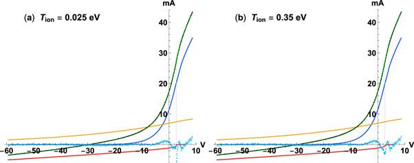
Figure 5. Experimental (black dots) and fitted (green trace) Langmuir probe I(V) characteristics acquired with the probe tip located 2 cm from the position of peak density and temperature for a helium plasma with the following engineering parameters (refer to table 1): Ip = 4.0 A, Pg = 6.0 mTorr, Vb = 89 V, Vf = 42 V, Ptot = 1.16 kW. The fitted cold (dark blue trace) and hot (orange trace) electron current characteristics correspond to fitted values of the respective electron densities and temperatures of  cm−3,
cm−3,  eV,
eV,  cm−3,
cm−3,  eV. These fitted values are identical, to within the quoted significant figures, for both panels. The red trace is the ion current characteristic, including both orbit motion-limited and charge exchange contributions. In the left-hand panel (a), Tion is fixed at the cold ion value of 0.025 eV. In the right-hand panel (b), Tion takes an optimally fitted value of 0.35 eV. The residuals
  scaled up by a factor of 10 are given by the light blue dotted profiles in each panel. The maximum residual magnitude in panel (b) is reduced by a factor of 1.8 relative to the maximum residual in panel (a).
Download figure:
Standard image High-resolution image4. Discussion
4.1. Fitting a single Gaussian to a temperature variation along a line of sight
The accuracy of the fit to spectral data, such as that plotted in figure 2, suggests that a single Gaussian line shape with an appropriately chosen width is, in practice, sufficient to describe the data. This is despite the fact that a superposition of Gaussian lines to account for a temperature distribution along the line of sight would be required to precisely fit noise-free data. Figure 6 shows two cases of simulated line integrals of Gaussian shapes where the temperature was chosen to vary by a factor of three from the edge to the centre of the line of sight, and the ion density is either uniform (figure 6(a)) or linearly rising from zero (figure 6(b)). See the caption for a description of the various traces.

Figure 6. Simulated line-integrated Gaussian profiles (blue traces, see equations (10) and (11) for analytical expressions) whose width variation along the line of sight corresponds to a factor of three variation in ion temperature, and whose amplitude is weighted by an ion density profile. (a): Uniform ion density. (b): Density climbs linearly from zero to a maximum value. The orange trace is the Gaussian profile corresponding to the minimum ion temperature Tmin at the edge of the plasma while the green trace corresponds to  at the centre. In each case, the red trace is a single Gaussian chosen so that its area coincides with that under the corresponding blue trace. Explicit expressions are given in equation (13).
Download figure:
Standard image High-resolution imageThe partially obscured blue traces in figure 6 were generated using an analytical approach (aided by Mathematica) as follows: the variable temperature Gaussian line shape was chosen to have a standard deviation  that varies linearly with a normalized spatial coordinate 0 ≤ z ≤ 1 along the line of sight from plasma edge to centre (symmetry about the plasma centre is assumed):

where  is the Doppler-broadened wavelength relative to λ0. Note from equation (3) that
  . Let
. Let  be the scale of temperature variation along the line of sight. A factor of
  variation in temperature is satisfied by the choice of σ0 = 1 and
  giving
  . For the uniform density profile
  assumed in figure 6(a), the ion density weighting function (normalized to n0) is w(z) = 1, and
  can be integrated to yield

The equivalent normalized profile is identical, since  . For the linearly rising density profile
  assumed in figure 6(b), the corresponding normalized integral, with normalization factor
  , is given by
where  is the exponential integral (the principal value of the integral is taken). If the weighted line-integrated variable width Gaussian expressions (10) and (11) are assigned the notation
  and
and  , then
  and
and  are plotted as the blue traces in figures 6(a) and (b), respectively.
A criterion for the closest equivalent single Gaussian shape G(σ, x) is that the area  under the curve be equal to the area under
  or
or  . Both these expressions can be analytically integrated to yield
  and
and  . Equating each of these results to
  yields σ(
 ) for the closest equivalent single Gaussian in the case of uniform and linearly rising density profiles:

The single Gaussians closest to the functions  and
and  by the criterion of equal area are accordingly given by

GU(3, x) and GL(3, x) are plotted as the red traces in figures 6(a) and 6(b), respectively.
A simple measure of the overall difference between  and
and  or
or  and
and  is the maximum difference between corresponding functions. The maximum difference in each case occurs in the vicinity of
  or
or  (see equation (12)). For the two examples in figure 6 where
  = 3, the maximum difference is
  for the uniform density profile and
  for the linearly rising profile. For the range 1 <
  ≤ 10 the maximum differences were recorded for both uniform and linear density profiles and the data were well fitted by the following Padé approximants for
  ≥ 2 , and a 5/3 power law for 1 ≤
  ≤ 2.
≤ 2.
These expressions, which are easily invertible to give  in each case, cover the ranges
  and
and  for the quoted variation in
  of 1 <
  ≤ 10. We also investigated the behaviour for large
  , of order 1000, and the maximum differences tended towards the asymptotic values of 0.16 and 0.075 for uniform and linear density profiles, respectively. These relations, illustrated by the close agreement between the blue and red traces in figure 6, support our experimental finding that the He II spectra, although extracted from a single line-integrated signal with variable Gaussian line width along the line of sight, could be accurately fitted assuming a pure Gaussian line shape. From these results, it is clear that the fitted ion temperature derived from each of the 162 experimental spectra corresponds to a lower estimate, in the region of 50%, of the maximum ion temperatures achieved at the hottest point in the plasma. Accordingly, maximum ion temperatures under the experimental conditions reported here are likely to have exceeded 0.5 eV.
4.2. Other points of discussion
All three fits in figure 3 have an approximately constant intercept of ≈ 0.125 eV and the question of spectrometer resolution naturally arises. The Bruker Vertex 80 has a wavenumber resolution of 0.08 cm−1, independent of wavenumber. This corresponds to a wavelength FWHM resolution of 8 × 10⁻⁹λ2 nm when λ is expressed in nm. For the He II lines of interest, the wavelength resolution evaluates to  pm at λ = 468.58 nm, and from equation (4) the corresponding temperature resolution is 0.0095eV. Hence we conclude that the approximately constant intercept for the regressions shown in the panels in figure 3 is not an artefact of finite instrument resolution.
The magnetic field strength B along the mirror axis, plotted in figure 7 for each magnet stack diameter, corresponds to the spatial profiles, plotted in figure 8, of the ion gyro-radius along the mirror axis, assuming a typical ion temperature of 0.2 eV. Note from figure 3 that, at a given value of the plasma current, the ion temperature increases with the magnet stack diameter. We can interpret this as follows: the decrease in the gyro-radius of the helium ions with increasing magnetic field strength results in a reduction in spatial diffusion and hence a longer residence time leading to increased energy equilibration with much hotter electrons, and thus to an increase in the ion temperature.

Figure 7. Magnetic field magnitude (log scale) as a function of position along the mirror axis for the 5 cm, 3 cm and 1.2 cm magnet stack diameters. The position of the inner walls of the vessel are shown by the dashed red lines. The minimum values at the mirror symmetry plane (indicated by the dashed grey line) are 16.2 mT, 5.9 mT and 1.0 mT for the 5 cm, 3 cm and 1.2 cm magnet stack diameters, respectively.
Download figure:
Standard image High-resolution image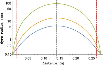
Figure 8. Singly ionized helium ion gyro-radius profiles (log scale) along the mirror axis assuming a 0.2 eV ion temperature for the 5 cm, 3 cm and 1.2 cm magnets stack diameters which, in the mirror symmetry plane (z = 0.14 m), take maximum values of 5.6 mm, 15.4 mm and 95.4 mm, respectively. The gyro-radius at the magnet face takes the same value of 0.15 mm for all three magnet stack diameters.
Download figure:
Standard image High-resolution image
Finally, it is noteworthy that the helium gas fill pressure was not selected in any of the optimised predictor models presented here. In particular, its low correlation with Tion apparent in table 2, where the maximum R2adj value is 0.146, is in stark contrast to that of the plasma current, the engineering variable most highly correlated with the ion temperature for the datasets from each of the three magnet stack diameters. It is likely that detailed transport simulations that lie outside the scope of this work would be necessary to find a quantitative explanation for these findings.
5. Summary and conclusions
The relationship between ion temperature and engineering parameters in a magnetic mirror helium plasma was investigated using Doppler-broadened emission lines of He II. The goal was to improve the quality of models used to fit Langmuir probe data where ions are usually assumed to be cold. A total of 162 high resolution He II spectra with plasma parameters randomly selected from a parameter space with four independent degrees of freedom were acquired and fitted, yielding ion temperature values in the range 0.07 eV–0.32 eV. We have demonstrated analytically that a line of sight signal with contributions from a range of Gaussian line widths can, in practice, be accurately fitted by a single Gaussian line shape. Because temperatures were derived from a single line-integrated signal, they correspond to lower estimates of the maximum temperatures established in the plasma. The single best predictor for the ion temperature for each of the three magnet stack diameters used here was the plasma current, and a linear regression model yielded root mean square fitting errors of 0.016 eV, 0.008 eV and 0.010 eV for the 1.2 cm, 3 cm and 5 cm diameter magnet stacks, respectively. A quadratic polynomial model in two predictors (with 6 free coefficients) improved these rmse values to 0.015 eV, 0.007 eV and 0.0055eV for the optimal two-predictor combination of plasma current and bias voltage. Further enlargement of the model to a quadratic polynomial in three predictors (with 10 free coefficients) yielded rmse values of 0.011 eV, 0.006 eV and 0.004 eV for the optimal three-predictor combination of plasma current, bias voltage and total heating power.
An increase in the magnet stack diameter causes an increase in the magnetic field magnitude everywhere within the plasma, thus reducing the gyro-radius. A reduction in the gyro-radius causes a decrease in ion diffusion across the magnetic field, and hence an increase in the confinement time of the ions—assuming the mean free path for collisions is longer than the gyro-radius. This, in turn, allows ions to absorb more energy from the electrons. This is consistent with the observed increase in the ion temperature with increasing magnet stack diameter for the same engineering parameters, and in particular for the same plasma current.
Acknowledgments
This work has been carried out within the framework of the EUROfusion Consortium in the context of the PhD project of the first author and has received funding from the Euratom research and training programme 2014–2019 under grant agreement No 633 053. The views and opinions expressed herein do not necessarily reflect those of the European Commission.