
Abstract
The plasma characteristics of atmospheric pressure micro-plasma jets in two different modes of excitation: low frequency (∼10 kHz), high voltage (∼15 kV) (LFHV) and high frequency (∼80 kHz), low voltage (4 kV) (HFLV), are investigated. The effect of AC electrical excitation on the plasma, depending upon wave amplitude and frequency, are looked at experimentally in the two systems. Plasma parameters such as the electron density (ne), electron excitation temperature (Texc), including optical line intensities from different species in the plasma are investigated as a function of applied external voltage, gas flow rate and operating frequency. Electrical modelling of the two different plasma systems are carried out and the results from the models are found to agree reasonably well with those of the experiments. It is found that the electron density and the temperature of the HFLV system are higher than the LFHV system at a particular gas flow rate, although the external applied voltage is higher for the LFHV system. A lower value of Texc for the LFHV system may make it suitable for medical or biological applications. Since a large electric field is created near the tip of the pin electrode in the HFLV system, therefore even though the applied voltage is lower than the LFHV system, the plasma can be easily generated. The HFLV system support a higher Texc, and such a system could be useful for material surface modification applications.
Export citation and abstract BibTeX RIS
1. Introduction
Atmospheric pressure plasma jets (APPJ) are cold plasmas created at atmospheric pressure. Unlike high temperature plasmas, these non-equilibrium plasmas have widely different ion (Ti) and electron (Te) temperatures, with the electron temperatures being about ∼0.5 eV and the ions are at room temperature ∼0.026 eV [1]. Due to their lower temperatures, the plasmas find many applications in areas such as biology [2–4], medicine [5–8], environment [9, 10] and in surface modification [11–15].
Based upon the application of AC electric fields, there have been quite a few methods to create atmospheric pressure plasma jets. Plasma jets with noble gases have been created with different configurations such as in dielectric free plasma jets (DFE jets) [16, 17], Dielectric barrier discharge jets (DBD jets) [18–22], DBD-like jets [23, 24], and single electrode (SE) plasma jets [25, 26]. In DFE jets, no dielectric material is used between the electrodes and the plasma is in direct contact with the metallic electrodes. On the other hand, DBD jets are created in a dielectric quartz tube and the electrodes are attached on the outer side of the tube. In DBD like jets, one of the electrodes is directly immersed in the plasma, and the SE jets are DBD-like without the ground electrode. However, there are hardly any experiments where the effect of wave amplitude and frequency on the plasma characteristics of the jet are investigated in two different jet configurations like the ones mentioned above.
In this article, the characteristics of the plasma in two different jet configurations are reported. In the LFHV configuration, the plasma jet is created as a DBD inside a dielectric capillary, with ring to ring electrode system, using high applied voltage (maximum 15 kV pp) but comparatively lower frequency (10 kHz), whereas in the second HFLV configuration, needle to ring electrode system is employed, which is a DBD-like jet and operates at a higher frequency (80–100 kHz) but lower voltages (0.6–4 kV pp). The plasma is characterized in the two systems and parameters such as electron density, electron excitation temperature, including optical intensities of the principal lines emitted by different species and radicals in the plasma are determined. Besides, the inter-electrode spacing is optimized and the variation of jet length as a function of applied voltage is investigated in the two systems. Additionally, to investigate the efficacy of application of the plasma jet in biological or medical systems, the creation of various reactive oxygen and nitrogen species (RONS) is investigated as a function of applied voltage and gas flow rate in both the systems. To further understand the discharge characteristics, particularly the power dissipated to the plasma jet, Lissajous figures are drawn and the power is determined. Both such plasma configurations have been widely employed in applications [27]. A knowledge of the plasma characteristics may be helpful in deciding the plasma system, depending upon the type of application. Besides looking at the plasma, electrical models have been developed for both the systems to understand the discharge characteristics.
The article is arranged as follows, in section 2, detailed descriptions of LFHV and HFLV experimental systems are presented. In section 3, measurement methodology and data analysis techniques, and in section 4, the experimental results are presented. Section 5 is on modelling of the two systems including a comparison of the results from the model and the experiments. Section 6 is on discussion of the experimental and modelling results. Finally, the results are summarized and conclusions drawn in section 7.
2. Experimental setup
The experiments have been performed with two systems: (a) Low frequency, high voltage (LFHV) system with the electrode configuration being ring to ring electrode and the second one (b) is a comparatively higher frequency, low voltage (HFLV) system.
In the LFHV system, a sinusoidal wave having maximum amplitude of 15 kV pp and 10 kHz frequency is used to produce the plasma inside a tapered capillary tube having inlet outer and inner diameters of 4.14 mm and 2.5 mm respectively, and outlet outer and inner diameters of 2.06 mm and 0.8 mm respectively. The capillary is wrapped with two aluminium tape electrodes having width of 4 mm. The high voltage electrode is located at 3 mm from the orifice of the capillary and the ground electrode is at 20 mm from the high voltage electrode in the upstream direction. The length of the plasma jet is approximately 10 mm. The range of the gas flow rate used in the experiments is 1–5 lpm (litres per minute).
In the HFLV system, needle to ring electrode configuration is employed, and the input voltage has a triangular wave form. The inner and outer diameters of the capillary are 3 mm and 5 mm respectively. The diameter of the high voltage tungsten pin electrode is 1.6 mm. The ground ring electrode is made of copper and its width is 5 mm. The applied voltage and frequency can be varied in the range 0.2–4 kV and 80–100 kHz respectively, and the gas flow is maintained in the range 3–5 lpm. In this study, the frequency has been maintained at 80 kHz. Figures 1(a) and (b) show the schematic diagram of the LFHV and HFLV systems, and the electrical waveforms of the typical input voltages for the two systems are shown in figure 1(c).

Figure 1. Schematic of (a) Low frequency (10 kHz), high voltage (0–15 kV pp) system (LFHV) which has ring to ring electrode system (b) High frequency (80 kHz), low voltage (1–4 kV) system (HFLV) which has needle to ring electrode configuration. (c) The waveforms of the input voltages in LFHV system at 11 kV (pp) and 10 kHz, and HFLV systems at 3 kV and 80 kHz. r and c denotes the ring electrodes and current monitors respectively.
Download figure:
Standard image High-resolution imageFigures 2(a) and (b) show the digital picture of the plasma jet in the LFHV and HFLV systems respectively. As can be seen from the digital pictures, the plasma jets in both the LFHV and HFLV systems are almost cylindrical and bright in the initial region and needle like at the tip. The typical jet lengths in the LFHV system is ∼1 cm and in the HFLV system is ∼2 cm. In the HFLV system the dielectric capillary tube and the electrodes are covered by a teflon tube. The working gas is helium with purity of 99.999%.

Figure 2. Digital picture of the plasma jet systems: (a) LFHV system at a gas flow rate of 2 lpm, voltage 10 kV (pp) and frequency 10 kHz (b) HFLV system at gas flow rate of 5 lpm, voltage 2.36 kV, frequency 80 kHz.The length is measured from 0 cm in the scale. The plasma jet starts after 5 mm distance from the high voltage electrode for the LFHV system as the capillary tube after the HV electrode can not be discernable in the picture.
Download figure:
Standard image High-resolution imageThe optical emission spectrum has been obtained by employing a high-resolution spectrometer (Andor Technologies, Shamrock 750) having two gratings (1200 and 1800 lines/mm) and a maximum resolution of 0.02 nm. An optical fiber (SR-OPT-8024) consisting of one channel with 19 UV/VIS fibres having 200 μm core diameter is employed to collect the light from the plasma.
Upon the application of the input voltage, when the voltage attains the gaseous breakdown threshold, ionization starts and the plasma is formed. Due to flow of gas, the plasma emerges out of the capillary in the form of a jet. Electrical measurements of the external and ground currents of the jet are carried out using Pearson current monitors (Pearson 4100) as shown schematically in figure 1(a) and (b), whose signals are taken to a Tektronix (DPO 4104) digital oscilloscope. The applied voltage is measured using a 1000 : 1 high voltage probe. During the experiments, the voltages have been varied from 9–14 kV for the LFHV system and from 0.6–4 kV for the HFLV system.
There are several methods to determine the electron density and temperature of a plasma. In general, Langmuir probes are employed for plasma diagnostics in low pressure plasmas, however, due to the limited size of the plasma jet (APPJ) and the plasma being highly collisional at atmospheric pressure, Langmuir probes may not be a suitable diagnostic system to determine the plasma parameters [28]. Other methods such as Thomson scattering, Rayleigh scattering have been used in various works [29]. In this work, the plasma characteristics have been determined by optical emission spectroscopy (OES) [30–35], which is a non-intrusive method. The electron density has been measured from the Stark broadening [36–39] of Hα and Hβ lines present in the spectrum and the electron excitation temperature has been measured using the Boltzmann plot method [40, 41]. As observed by many authors [36, 37, 39, 40, 42], it has been found that using only the Lorentzian fitting of a single Hα or Hβ line leads to an overestimation of the electron density by as much as an order, because of not incorporating the Van der Waal broadening which is significant at lower gas temperatures and needs to be subtracted out. However, using a difference technique [43] of the Lorentzian for both Hα and Hβ lines, helps to eliminate the effect of the Van der Waal broadening. Both these techniques will be discussed in the next section.
The electron densities have been measured at different voltages and frequencies in the HFLV system, where there was a possibility of varying the applied voltage over a small range of frequencies, but in the LFHV system, the density was measured at a particular frequency, as this system allowed a single frequency operation.
3. Measurement and analysis
The electron excitation temperature Texc is determined by the Boltzmann plot method as partial local thermodynamic equilibrium (PLTE) can be expected in these plasmas [44]. Usually in atmospheric pressure plasmas, the ion temperature Ti ≈ Tg, where Tg is the gas temperature. However, Te, Ti and Texc are not all equal to each other as observed in a plasma in thermodynamic equilibrium, and take different values, usually Texc < Te [45]. In this work, the Texc as determined by the Boltzmann plot method is described below [46].
When an atom gets de-excited from an upper energy level (k) having energy Ek to a lower energy level (i) having energy Ei, the emission coefficient of the spectral lines can be expressed as

where, h is the Planck's constant, c is the velocity of light in vacuum, Aki is the transition probability, λki is the wavelength of transition of the atom from the upper level k to the lower level i and Nk is the atom density in the upper level. Nk can be expressed as,

where, N is the total population density, Z(T) is the partition function which describes the sum of Boltzmann functions for all energy levels, and gk is the statistical weight factor of the upper level k. After substituting equation (2) in equation (1) and rearranging, we obtain

and taking logarithm on both sides, we finally obtain,

The temperature T in equation (4) represents Texc and can be evaluated from the slope of a plot between  and energy Ek. The values of Aki and gk are taken from NIST data base [47], where C is a constant.
The electron density has been determined from the Stark broadening of the Hα and Hβ lines present in the spectrum. To observe the Stark broadening, hydrogen Balmer lines (Hα and Hβ) are most suited because the Stark effect is linear [42] on these lines and electron density can be calculated from the individual Stark broadenings of both the lines [38, 43, 48]. There are different advantages and disadvantages of using these two lines [48]. Furthermore, the electron density can vary based on different methods such as Kepple-Griem theory (KG) [49] and computational model of Gigosos-Cardeñoso (GC) [49]. However, the KG theory overestimates the electron density by about 22% (Hβ) and 80% (Hα) with respect to the GC model. The computation results of GC model have better agreement with experimental results. The experimental data of the Hα and Hβ lines follows the Voigt profile which is a convolution of Gaussian and Lorentzian profiles. Therefore, the full width at half maximum (FWHM) of the Gaussian (wG) and Lorentzian profiles (wL) contributes to the FWHM of the Voigt profile. It is known that Stark (wS) and Van der Waal (wW) broadening contribute to the Lorentzian profile [43]. On the other hand, Doppler (wD) and instrumental (wA) broadening contribute to the Gaussian profile. Therefore, the FWHM of Gaussian broadening can be expressed as [50],

The Lorentzian part of the broadening in the Voigt profile can be deconvoluted from the measured FWHM (w0) of the Voigt profile as,

The electron density is normally determined from the Stark broadening component of the Lorentzian part of the FWHM [43, 48]. Although, Stark broadening dominates the Lorentzian part, however at lower temperature of the gas (below 500 K) the Van der Waal broadening becomes prominent [51]. The Lorentzian part for Hα and Hβ can be written as follows [43]


It is known that the Van der Waals broadening is related to the gas temperature Tg by the expressions [51]


where,  , and α is the polarizability of the perturbed atom in cm3, P is the pressure measured in atm, and μ is the reduced mass of emitter and ion pair. From equation (9) and (10) when Tg is very low, the contribution of the Van der Waal broadening to the Lorentzian part of FWHM is larger. It has been found that the calculation of the electron density only from the Lorentzian part of the broadening leads to an overestimation of the electron density, because of the error induced due to the neglect of the Van der Waal broadening. There are reports that explain when the gas temperature is lower than 500 K, the overestimation [51] could reach up to 500%. To reduce the error in the estimation, the electron density has been calculated from the difference between the Lorentzian part of the Hα and Hβ lines [50] and is given by,

where, R(Tg) is the difference between the Van der Waal broadenings. R(Tg) becomes negligible (about 5% of the difference of the Lorentzian) at a gas temperature of 1000 K. Hence, the difference between the Lorentzian profiles of the two lines (Hα and Hβ) becomes independent of Van der Waals broadenings. Finally, the electron density can be estimated from the expression below [51],

4. Experimental results
Figure 3 shows the optical emission spectrum for both the systems in the wavelength range 330–780 nm. Interaction between energetic electrons and helium metastable (Hem) state with the molecules of ambient air can produce different spectral lines as observed in the experiments. Several emission lines are observed and amongst them the most intense line is He I (706.5 nm) for both the systems. The intensities are therefore normalized with respect to 706.5 nm. The principal emission lines observed are N2 (337.1 nm),  (391.4 nm), He I (706.5 nm, 501.6 nm and 587.6 nm), O (777.3 nm) and Hα (656.3 nm) lines. It can be seen from the two spectra that the relative intensity (as compared to that of He I (706.5 nm)) of N2,
  , O (777.3 nm), and Hα lines are more intense for the HFLV system (figure 3(b)) under the operating conditions. The different transitions and wavelengths of the lines are summarized in table 1.

Figure 3. (a) Optical emission spectrum of LFHV system (Gas flow rate : 2 lpm, voltage: 13 kV, frequency: 10 kHz) (b) Optical emission spectrum of HFLV system (Gas flow rate: 5 lpm, voltage: 2.52 kV, frequency: 80 kHz).
Download figure:
Standard image High-resolution imageTable 1. Principal lines of plasma emissions.
| Spectral lines | Wavelength (nm) | Transitions | |
|---|---|---|---|
| Nature | Species | ||
| Molecular | N2 | 337.1 |

|
| Ionic |

|
391.4 |
|
| Atomic |

|
486.1 |

|
| Atomic | He I | 501.6 |

|
| Atomic | He I | 587.6 |

|
| Atomic |

|
656.3 |

|
| Atomic | He I | 667.8 |

|
| Atomic | He I | 706.5 |

|
| Atomic | He I | 728.1 |

|
| Atomic | O | 777.3 |

|
As mentioned above, Hα and Hβ lines of hydrogen Balmer series are important for the measurement of electron density of the plasma. Figure 4 shows the relative intensity of Hβ lines with respect to Hα lines for both the systems. It is interesting to note that the relative intensity of Hβ line is higher for the HFLV system.
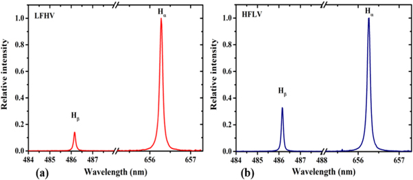
Figure 4. Relative intensities of Hβ lines with respect to Hα lines of (a) LFHV system at voltage: 13 kV, flow rate: 2 lpm, frequency: 10 kHz, and (b) HFLV system at voltage: 2.52 kV, flow rate: 5 lpm, frequency: 80 kHz.
Download figure:
Standard image High-resolution imageFigure 5 shows the variation of discharge current and intensity of the optical lines with inter-electrode spacing for the LFHV system. When the distance between the electrode increases, it seems after 2.5 cm, both the intensity and discharge current increases. However, the plasma becomes unstable at inter electrode spacing ≥2.5 cm. Hence, we have considered 2 cm as an optimised distance in case of LFHV system. The system has been optimized at 2 cm inter-electrode spacing by considering the discharge current and optical intensity of the important spectral lines. In the HFLV system, the inter-electrode spacing is fixed.

Figure 5. Variation of (a) discharge current and (b) line intensities with inter electrode spacing for the LFHV system at a voltage of 14 kV, flow rate 2 lpm and frequency 10 kHz.
Download figure:
Standard image High-resolution imageFigure 6 shows the variation of plasma jet length with the applied external voltage. With the increase of voltage, the jet length increases for both the systems. For the LFHV system, the jet length increases until ∼1 cm and stays constant with further increase in voltage. For HFLV system, jet length increases until 2.5 cm with the increase in voltage.

Figure 6. Variation of jet length of the LFHV system (at 2 lpm and 10 kHz) and HFLV system (at 5 lpm and 80 kHz) with applied voltage.
Download figure:
Standard image High-resolution imageAs mentioned earlier, the electron excitation temperature (Texc) has been calculated by the Boltzmann plot method. Five helium atomic lines (He I) have been chosen for this purpose, namely 501.6 nm, 587.6 nm, 667.8 nm, 706.5 nm, and 728.1 nm. Figure 7(a), shows the relative optical intensity of these lines as a function of applied voltage for the LFHV system. The optical intensities are normalized with the maximum value of the He I line at 706.5 nm occurring at 11.5 kV for LFHV system and at 2.52 kV for HFLV system respectively. It is noted that the intensity of the emission lines increases with increase in applied voltage, with a maximum intensity being around 11.5 kV for the LFHV system, however, the increase is found to be largest for the 706.5 nm line. After ∼12 kV the intensities stay almost constant. For the HFLV system, the relative intensity of these lines with applied voltage is shown in figure 7(b). Here the voltage is varied in the range 1.6–3.6 kV. In this system as well, we observe that the optical intensity is largest for the 706.5 nm line. The intensities peak around 2.8 kV, although for the 706.5 nm line the peak occurs much earlier ∼2 kV.

Figure 7. Variation of intensity of different helium lines with applied drive voltage for the (a) LFHV system (Gas flow rate : 2 lpm, frequency: 10 kHz), and (b) HFLV system (Gas flow rate: 5 lpm, frequency: 80 kHz).
Download figure:
Standard image High-resolution imageFigure 8 shows the variation of the electron density with applied voltage for both the systems. In general, the electron density is seen to increase with increase in applied voltage for both the systems. It can be seen that the electron density is somewhat higher for the HFLV system, although the operating voltage is much lower than the LFHV system. The average increase in density is 9% per 1 kV for LFHV and ∼90% for HFLV systems after 3 kV, as shown in figure 8(a) and (b) respectively. The fitting equations are provided in table 2.

Figure 8. Variation of electron density in (a) LFHV system at a flow rate of 2 lpm and at 10 kHz and (b) HFLV system at a flowrate of 5 lpm and at 80 kHz.
Download figure:
Standard image High-resolution imageTable 2. Fitting equations for the electron density (ne) variation with voltage and gas flow rate. These equations are applicable for input voltages in the range 9–14 kV and 1.76–3.78 kV for the LFHV and HFLV systems respectively. The gas flow rate ranges are 0.5–5 lpm and 2.5–5 lpm for the LFHV and HFLV systems respectively. Electron density ne is in 1013 cm−3, voltage (V) is in kV and the flow rate (L) is in lpm.
| LFHV | HFLV | |
|---|---|---|
| 10 kHz | 80 kHz | |
| Density with voltage (V) |

|

|
 , and t = 4.5 , and t = 4.5 |
 , and t = 0.83 , and t = 0.83 |
|
| Density with gas flow rate (L) |

|

|
 , and t = 0.63 , and t = 0.63 |
a = 2.45 and 
|
Figures 9(a) and (b) show the variation of the electron excitation temperature with the applied voltage and gas flow rate for the LFHV and HFLV systems. It is seen that with increase in flow rate,  decreases for both the systems, as expected. Although, the range of the gas flow rate is different for both the systems, it is observed that beyond a certain gas flow rate (∼2.4 lpm for the LFHV system and ∼3.75 lpm for the HFLV system) Texc tends to be almost constant. Figure 9 also shows the variation of Texc with applied voltage. Texc seems to decrease exponentially with voltage for both the systems. The fitting equations are provided in table 3.

Figure 9. Variation of electron excitation temperature of (a) LFHV system for varying applied voltage (gas flow rate is fixed at 2 lpm) and varying gas flow rate (voltage is fixed at 14 kV) for a fixed frequency of 10 kHz and (b) HFLV system for varying applied voltage (gas flow rate is fixed at 5 lpm )and at 80 kHz and for varying flow rate (voltage is fixed at 3 kV and frequency is fixed at 80 kHz).
Download figure:
Standard image High-resolution imageTable 3. Fitting equations for the electron excitation temperature (Texc) with applied voltage and gas flow rate. These equations are applicable in the range 9–14 kV and 1.75–3.8 kV for the LFHV and HFLV systems respectively. The gas flow rate ranges are 0.5–5 lpm and 2.5–5 lpm for the LFHV and HFLV systems respectively. Texc is in eV and voltage is in kV.
| LFHV | HFLV | |
|---|---|---|
| 10 kHz | 80 kHz | |
| Texc with voltage (V) |

|

|
 , and t = 0.13 , and t = 0.13 |
 , and t = 0.38 , and t = 0.38 |
|
| Texc with gas flow rate (L) |

|

|
 ,and t = 0.62 ,and t = 0.62 |
 , and t = 0.62 , and t = 0.62 |
Figures 10(a) and (b) show the variation of plasma electron density with gas flow rate. It is interesting to note that the decrease is exponential for the LFHV system and almost linear for the HFLV system. The fitting equations for figure 10 are provided in table 2.

Figure 10. Variation of the electron density with gas flow rate for the (a) LFHV system (14 kV pp) and 10 kHz (b) HFLV system at frequency: 80 kHz, voltage: 3 kV.
Download figure:
Standard image High-resolution imageFigures 11(a) and (b) show the variation of the optical intensity of the emission lines (501.6 nm, 587.6 nm, 667.8 nm, 706.5 nm, and 728.1 nm) with the gas flow rate. The intensity is normalized with the line intensity of 706.5 nm line at 4.5 lpm for both the systems. While most of the lines show an increase in the optical intensity, the line at 706.5 nm shows a remarkable increase in the intensity with flow rate, which is significantly higher than the other emission wavelengths.

Figure 11. Variation of optical intensity with flow rate for different helium lines (501.6 nm, 587.6 nm, 667.8 nm, 706.5 nm, and 728.1 nm) for (a) LFHV system (Voltage: 13 kV pp, frequency: 10 kHz) and (b) HFLV system (Voltage: 2.52 kV, frequency: 80 kHz).
Download figure:
Standard image High-resolution imageFigure 12 shows the intensity variation of RONS with applied voltage and gas flow rate for the LFHV sytem. The reactive species which have been investigated are OH (308 nm), NO (282.9 and 289.2 nm), and atomic oxygen (777.3 and 844.4 nm). It can be seen that the intensity of the RONS increases with the increase of gas flow rate and applied voltage. It seems that with increase in applied voltage and gas flow rate, the generation of OH (308 nm) and O (777.3 nm) increases very rapidly and almost equally for the LFHV system in comparison to other RONS, whereas for the HFLV system, OH does increase more than the rest of the species but the increase in O is comparatively less. Similarly, figure 13 shows the intensity variations of the RONS with voltage and flow rate for the HFLV system.

Figure 12. Variation of optical intensity of different reactive species with (a) voltage at 2 lpm and 10 kHz frequency and (b) flow rate at 14 kV and 10 kHz frequency of the LFHV system.
Download figure:
Standard image High-resolution image
Figure 13. Variation of optical intensity of different reactive species with (a) voltage at 2 lpm and 10 kHz frequency and (b) flow rate at 14 kV and 10 kHz frequency of the HFLV system.
Download figure:
Standard image High-resolution imageDissipated power to the plasma jet has been calculated by drawing the Lissajous figure for both the systems as shown in figure 14. Also, the variation of power with the applied voltage and gas flow rate has been shown in figure 15 for both the systems. The discharge power increases with the applied voltage but it decreases with the gas flow rate.

Figure 14. Lissajous figure at (a) V = 14 kV (pp), flow rate = 2 lpm, frequency = 10 kHz and power 0.7 W for LFHV system and at (b) V = 1.1 kV (pp), flow rate = 5 lpm, frequency = 80 kHz and power 0.2 W for HFLV system.
Download figure:
Standard image High-resolution image
Figure 15. Variation of discharge power with voltage and flow rate of (a) LFHV system (parameters: flow rate = 2 lpm (when applied voltage varies), V = 14 kV (when flow rate varies), f = 10 kHz) (b) HFLV system (parameters: flow rate = 5 lpm (when voltage is varied ), V = 1.1 kV (pp) (when flow rate is varied ), f = 80 kHz).
Download figure:
Standard image High-resolution image5. Electrical modelling
An electrical model is employed to understand the nature of the internal discharge current and the results of the model are compared with the experimental results. Both the systems have been replaced by the equivalent electrical components [50]. The capacitance is calculated for the dielectric quartz tube and the gas by using the parallel plate capacitance method. For the LFHV system, the capacitance of the dielectric tube is calculated to be 1.33 pF and the gas capacitance to be 0.0174 pF, and for the HFLV system, the dielectric tube capacitance and gas capacitance are 2.5728 pF and 0.417 pF respectively. The temporal variation of the internal discharge current is obtained from [52].

where, Idis(t) is the current calculated when the discharge occurs inside the capillary tube, Cg is the capacitance of the gas, Cd is the capacitance of the capillary tube, Iext(t) is the external current which includes both the displacement current with plasma off and the conduction current with plasma on, and Uext(t) is the externally applied voltage.
Figure 16(a) and (b) shows a schematic of the electrical circuit for the two systems. When the plasma is formed inside the capillary the medium inside the capillary changes. To remove the complexity of the system, the plasma between the two electrodes has been replaced by a constant gas capacitance (Cg) and a voltage controlled current source [52].

Figure 16. Equivalent electrical model of the (a) LFHV and (b) HFLV systems.
Download figure:
Standard image High-resolution imageFigure 17(a) shows the waveform of the externally applied voltage Uext(t), the experimentally obtained external current Iext(t) with plasma on and the external current without plasma which is mainly the displacement current. In figure 17(b), the calculated current between the two electrodes with the plasma on Idis(t) has been plotted with Iext(t) for the LFHV system. During the rising and falling of voltage signal a peak is observed in the external current, which indicates the plasma formation inside the capillary tube. Idis(t) has been calculated using equation (13). It is noted that the calculated and experimental results match reasonably well.

Figure 17. Plot of (a) external applied voltage (Uext(t)), external current (Iext(t)) with plasma on and off and (b) the calculated current between the two electrodes (Idis(t)) and external current with plasma on for LFHV system at voltage: 12 kV, frequency: 10 kHz, gas flow rate: 1 lpm.
Download figure:
Standard image High-resolution imageFigure 18(a) shows the waveform of the externally applied voltage Uext(t), the experimentally obtained external current Iext(t) with plasma on, the external current without plasma which is mainly the displacement current for the HFLV system. In figure 18(b) the calculated current between the two electrodes with the plasma on Idis(t) has been plotted with Iext(t) for the HFLV system. In this case, we observed two sharp peaks of current at the falling edge of the voltage pulses. Here also, Idis(t) has been calculated using equation (13). The wave form of the voltage is different than the LFHV system, it acts as a unidirectional voltage pulse. When the voltage pulses reach the maximum value a primary discharge is observed and we obtain the first peak. The next current peak is a result of a secondary discharge.

Figure 18. Plot of (a) external applied voltage (Uext(t)) along with external current (Iext(t)) with plasma on and off and (b) the calculated current between the two electrodes (Idis(t)) and external current for the HFLV system at voltage: 3 kV, gas flow rate: 3 lpm, frequency: 80 kHz.
Download figure:
Standard image High-resolution image
6. Discussion on the experimental results and electrical modelling
In both LFHV and HFLV systems, high energy electrons can be produced during rise time of the high voltage pulse. As the voltage is increased, more atoms get ionized and eventually electron density increases as shown in figure 8 and these electrons are responsible for exciting the atoms to its higher states. When these excited atoms return back to ground state, light is emitted from these transitions and the intensity of the emission lines increases with applied voltage until a certain value of the voltage, depending upon the gas flow rate for both the systems as shown in figure 7.
In figure 8, it is shown that the electron density increases with voltage for both systems but the value of electron density is more for the HFLV system, even though it has a lower input voltage. The LFHV system is a DBD jet while the HFLV system is a DBD-like jet in which the needle electrode is directly in contact with the plasma. When the high voltage is applied to the needle electrode, the electric field at the tip of the electrode can become quite high, therefore even though the applied voltage is lower, gaseous breakdown can happen easily in the HFLV system. Additionally, the high voltage surface area of the central conductor is larger than that of the ring electrode surface area of the LFHV system. When the frequency of the power supply increases, the electron-neutral collision frequency increases, hence the electrons lose their energy to the neutral atoms. The trend of electron density variations follows the trend of power variation for both the systems (cf figure 15).
With increase in the applied voltage the electron excitation temperature tends to remain almost constant or even decrease as observed for the HFLV system (cf figure 9). The absorbed power by the electrons could be spent in ways such as to bring about ionization or atomic excitations and thereby lose its energy. In the present experiment, since the plasma is highly collisional, the energy carried by the electrons is expected to be primarily spent in atomic excitations. It appears that increasing the applied voltage primarily increases the electron density and these electrons redistribute the electric field inside the plasma jet and weaken the electric field inside the jet. The energy exchange between the field and the charged particles weakens [37].
When the flow rate increases, the neutral pressure inside the capillary increases and because of the enhanced rate of collisions between the electrons and the gas atoms, the electrons lose its kinetic energy, thereby decreasing the electron excitation temperature. Additionally, charged particles are not able to gain enough energy to ionize the gas further. Therefore, the electron density decreases with increase in gas flow rate as seen in figure 10. In figure 11(a) and (b), the intensity of the lines increases with the gas flow rate, this may in general occur because of the increase in the neutral density which increases the excitation and de-excitation rates.
In figure 12 and 13, it is shown that the intensity of the reactive oxygen and nitrogen species (RONS) increases with the increase of flow rate and applied voltage. Energetic electrons or long lived helium metastable (Hem) states create these RONS. It has been reported that intensity of NO is more in the turbulent flow of the plasma jet [53]. The radicals are produced by the following reactions.
The above mentioned species are reactive and can be lethal for micro organisms [54]. In the modelling results, when the gap voltage between the two electrodes inside the capillary becomes more than the threshold voltage for gaseous breakdown, plasma is ignited inside the tube and the charges accumulate on the inner surface of the dielectric tube, which eventually reduces the gap voltage inside the capillary tube and the plasma extinguishes. In every positive and negative part of the signal we can observe such a sharp peak of current due to the discharge (cf. Figure 17). The charges which accumulate on the inner surface of the capillary tube do not let the gap voltage increase beyond the breakdown voltage between the two electrodes inside the capillary. These charges are called memory charges in dielectric barrier discharges. The accumulated memory charges help the next discharge to occur at a lower voltage than the first value of ignition voltage of external applied voltage. In case of the HFLV system, because of the secondary discharge peak (cf figure 18), no memory charges are left on the capillary tube before the next pulse. This is called 'self-erasing' effect for the unidirectional voltage pulse in DBD discharge [52].
7. Summary and conclusions
In this study, the spectral intensity of different species, including plasma parameters such as ne and Texc have been measured in atmospheric pressure micro-plasma jets in two different modes of drive excitation, corresponding to frequency and voltage modes. It is observed that the intensity of the different spectral lines increases with applied voltage and gas flow rate. With increase in the gas flow rate, the electron density decreases for the LFHV and HFLV systems. On the other hand, Texc decreases for both the systems with increase in gas flow rate. At a fixed gas flow rate, ne increases for both the systems with increase in applied voltage, however, Texc initially decreases sharply and remains almost constant.
The creation of RONS have been investigated. The line intensity of these reactive species has been measured with applied voltage and gas flow rate. The amount of RONS can be manipulated by varying applied voltage and gas flow rate. The number density of RONS increases with gas flow rate and becomes constant after a certain gas flow rate for both the systems. With the increase in applied voltage, the number density of RONS increases.
Additionally, the variation of jet length has been investigated with applied voltage for both the systems and the LFHV system has been optimized with inter electrode spacing. Power has been measured for both the systems. HFLV system produces longer jet length with comparatively lower applied voltage and the discharge power is also lower than LFHV system, although the requirement of gas flow rate is higher. On the other hand, LFHV system requires higher external voltage to produce the jet and length of the jet is smaller than the jet length of the HFLV system, but the requirement of gas flow rate is lower.
The performance of both the plasma jet systems under the influence of different parameters have been investigated in this article. In the LFHV system, the discharge power is higher than the HFLV system, but the requirement of gas flow to achieve similar electron density and electron excitation temperature is lower than the HFLV system. The HFLV system operates well in the higher gas flow rate regime than the LFHV system. The LFHV system has the higher discharge power but the Texc for this system is lower, therefore, it could be used for biological applications. On the other hand, the HFLV system has the lower discharge power but Texc is higher. A large electric field is created near the tip of the pin electrode, therefore, even if the applied voltage is lower than the LFHV system, the plasma can be easily generated. It could be useful for surface modification applications. Electrical modelling of the two systems helps us to obtain a true measure of the discharge current inside the plasma. By studying the plasma parameters in the two different configurations and modes of excitation, we can select the most efficient system according to the desired application.
Acknowledgments
We sincerely acknowledge the Board of Research in Nuclear Sciences, Government of India (Sanction no: 39/14/33/2016-BRNS) for funding this research. SB gratefully acknowledges support from a Sanjay and Rachna Pradhan Chair Professorship. Fruitful comments by Prof. Manas Khan and Prof. Supratik Banerjee, IIT Kanpur are gratefully acknowledged. We sincerely thank the anonymous referees for their valuable comments which has enriched the work. We would also like to thank Mr C. Patil and Mr A. Visani of FCIPT, IPR, Gandhinagar, for their help in installing the HFLV system. We thank the Central workshop and Physics workshop, IIT Kanpur for their help in fabrication of experimental components.