
Abstract
We discuss the relativistically covariant ponderomotive effect of a spin-less electron by a high-intensity laser field of a plane wave in the quantum regime. At first we recall the relativistic ponderomotive effect in classical mechanics. Then against that, we will investigate quantum mechanical expression of the ponderomotive effect by relativistic stochastic mechanics, where, we also propose relativistic stochastic mechanics to draw a trajectory of a spin-less electron. After giving a strict solution of stochastic mechanics, its slowly varying motion is examined as its ponderomotive effect in the quantum regime. Finally, we will see the universality of the ponderomotive effect acting on a spin-less electron interacting with a present high-intensity femtosecond laser, via the dressed (effective) mass of a spin-less electron bridging between classical and quantum mechanics.
Export citation and abstract BibTeX RIS
1. Introduction
In recent years, plasma physics assisted by intense electromagnetic fields has been investigated by high-intensity laser facilities [1–6] in the world. Its typical idea is irradiation of high-intensity laser beams on several types of targets. When a target material is irradiated by such a high-intensity laser, it is expected that electrons are emitted from atoms in that target material due to a tunneling-ionization process [7]. Those free electrons may be accelerated up to the speed of light when a field intensity of a background laser field is larger than 1018W/cm2. Let us consider a classical equation of motion of a free electron in a laser field briefly:  with
with 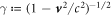 ,
,  and
and  for
for 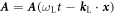 as a laser field of an angular frequency ωL and a wave vector
  . Where,
  ,
,  and c are the rest mass, charge, velocity of an electron and the speed of light, respectively. For instance,
  at t = 0. The following is derived from the above equation of motion (we will see its 4-vector form later):

Where,  , the time average of the non-linear force
  for a single laser circle 2π/ωL, is the so-called ponderomotive force in plasma physics [8–10]. We regard
  as a slowly varying part of
  in this article, abstractly. When we consider ωL is large enough,
 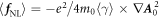 for
for  . The non-linear force
  corresponds to
  . Generally speaking, the factor
  is non-zero even in the rest frame of an electron. An appearance of large enough
  is regarded as a signature of the relativistic regime since
  becomes zero in the non-relativistic regime. Thus, the ponderomotive effect due to
  is treated as one of the research topics in relativistic laser-electron interactions. The force
  is a vector parallel to
  since
since  is a function of
  . This is the reason why a high-intensity laser field accelerates an electron to the positive direction of
  relativistically [11]. The ponderomotive effect is applied to the plasma channeling and the ponderomotive self-focusing effect [12–14], the laser wake field acceleration method [15–17], the hole boring effect [18], etc.
An electron has to be expressed as a relativistic and quantum mechanical object in non-linear and quantum processes by high-intensity lasers [1–6, 19, 20]. It is necessary to describe the ponderomotive force acting on an electron in relativistic quantum mechanics, too. In fact, non-linear processes in quantum electrodynamics are expressed by an electron dressing a high-intensity laser field. We can see this via the ponderomotive effect in classical dynamics: the ponderomotive effect is regarded as a propagation of an electron dressing a laser field. We will see that detail in the mass correction

The existence of meff suggests that an electron dresses an additional mass  due to a laser field. The contribution of δ m cannot be omitted in general, even in the case of the rest frame.
In this article, we investigate the relativistic ponderomotive effect in relativistic stochastic mechanics as quantum mechanics. Let us explain the importance on the relativistic covariance of equations. This is the reason why that covariance ensures to use the Lorentz transformation. Our idea consists of two problems. The first issue is to decide the definitive edition of the relativistically covariant ponderomotive force acting on a classical and spin-less electron. We will confirm that by solving equation (3) strictly with an external laser field of a plane wave in section 2, though there are several proposals of the relativistic models [21–23]. We extract a slowly varying component from the strict solution, as the ponderomotive effect. Kibble's form [21, 22] is derived as a result of that and this is the preparation for the later discussion in the quantum regime. The second problem is how we can express the ponderomotive effect in relativistic quantum mechanics. Let us formulate it by stochastic mechanics developed by E. Nelson [24, 25]. Stochastic mechanics is a formulation of quantum mechanics by stochastic analysis. We introduce its basic strategy in section 3. We hereby expand stochastic mechanics from Nelson's model in the non-relativistic regime to a relativistically covariant model: a quanta draws a 4D stochastic process  as its trajectory given by stochastic kinematics
  with dynamics
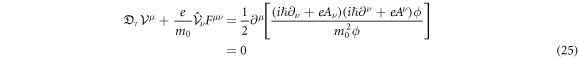
 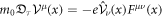 . We define this dynamics as the Klein-Gordon (KG) equation of a spin-less electron.Stochastic mechanics is the unique method to illustrate a realistic trajectory of a particle in quantum mechanics. It is expected to employ the same method of classical mechanics in the quantum regime since stochastic mechanics has both kinematics and dynamics. The ponderomotive effect in stochastic mechanics is discussed in section 4. It becomes one of few applications of stochastic mechanics. The ponderomotive effect is described by a physical process satisfying the following KG equation:
  . We will confirm this naive result by stochastic mechanics. The readers may find the fact that the ponderomotive effect in the quantum regime is not so different from one in the classical regime described by section 2, except randomness in the present model. Especially, the effective mass correction should be taken into account in both regimes. This is the signature that the ponderomotive effect acts on a charged particle in both classical and quantum mechanics universally. Once again let m0 and
  be the rest mass and charge of a spin-less electron.
2. Classical regime
Let us derive the relativistic ponderomotive effect in classical mechanics. Hence, we only deal with the basic equation of motion

for a spin-less electron in this section. Equation (3) is equivalent to  as its 3D expression. Where,
  is a 4-velocity of a spin-less electron and F is an electromagnetic field tensor characterized by
  with a 4-potential A of a laser field. We also introduce the metric
  for
for  . Recall v satisfies v · v = c2 due to this metric. Suppose the external field of a laser beam is a plane wave, i.e., A = A(k · x) for a 4-wave vector
  . Let the laser field be now
  with
with  . We set the Lorenz gauge condition ∂μAμ = 0 and the initial condition A(θ(0)) = 0 for
  , too. Under such a laser field of a plane wave, equation (3) has its exact solution below [26]:
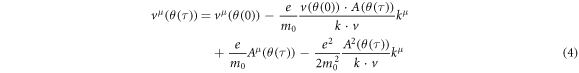
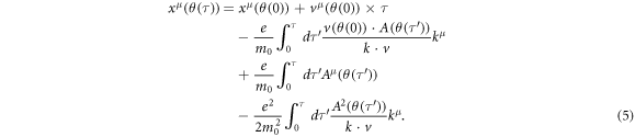
We wrote v(θ(τ)) = v(τ) for our readability. Since v = dx/dτ, an electron draws
Where,  is a Lorentz invariant since
  . The readers may find

by using equation (4). Since d/dτ = k · v × d/dθ(τ),


is derived strictly as the one equivalent to equation (3). The non-linear force  is extracted from the Lorentz force
  in equation (3). We remark equations (7)–(8) do not require any assumption except an external laser field of a plane wave. We just transformed the exact solution of equation (3). Let
  be a slowly varying part of
  , i.e.
  omits rapidly oscillating components like ωL and its harmonics in
  . Consider the operation of
  wrt Equations (7)–(8):

Equation (9) gives the slow components of equations (4)–(5):


With  and
and  as the initial conditions.
 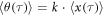 as the index of
  is also corrected from θ(τ) here. Equation (11) represents a trajectory of a slowly varying motion of a spin-less electron. We can confirm the 3D form of equation (9): since
  and
and  , equation (9) becomes

with  . This is an equation of a slowly varying motion w.r.t. Equation (1).
The force  in equation (9) may be considered as a relativistically covariant ponderomotive force. However, we still cannot suggest that since its time component
  is unclear and
 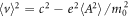 due to equation (10). The operation
  acting on equation (3) implies
  . We can recover that squared velocity rule by the method of T. W. B. Kibble [22]. Suppose
 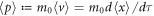 ,
, ![$\langle p{\rangle }^{2}={m}_{0}^{2}[1-{e}^{2}\langle {A}^{2}\rangle /{m}_{0}^{2}{c}^{2}]{c}^{2}$](https://content.cld.iop.org/journals/2516-1067/1/2/025011/revision1/prexab1719ieqn64.gif) . Then, we define the effective mass
. Then, we define the effective mass

and introduce a new proper time τeff such as 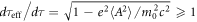 . Let
. Let  , we obtain
 ![${[d\langle X\rangle /d{\tau }_{\mathrm{eff}}]}^{2}={c}^{2}$](https://content.cld.iop.org/journals/2516-1067/1/2/025011/revision1/prexab1719ieqn67.gif) and
and

which gives  . Then, the following is the relativistically covariant equation of a slowly varying motion of a spin-less electron in a high-intensity field:

Consider  as a conservative force, then,

is the so-called ponderomotive potential in the relativistic covariant form. Equations (13), (15) for  are equivalent to equation (9) for
  because both expressions derive the same solution of equation (11). We hereby conclude that the relativistically covariant equation of motion for the ponderomotive effect is expressed by equation (15) with the effective mass of equation (13).
3. Relativistic stochastic mechanics
Stochastic mechanics is one of formulation of quantum mechanics by using stochastic analysis. Its non-relativistic model was completed by E. Nelson [24, 25] with the following achievements: (A) it is equivalent to the Schrödinger equation, (B) it has stochastic kinematics to draw a trajectory of a quanta and (C) Born's rule is naturally satisfied in this model. Especially, the ability-(B) is useful to confirm the classical-quantum correspondence of the ponderomotive effect. We investigate its relativistic version for that purpose since a high-intensity laser accelerates a spin-less electron to nearly the speed of light. Though the several authors had proposed each relativistic models [27–30], however, its definitive edition has not been found. There is no practice to draw a trajectory by them, too. Here we propose a new model of relativistic stochastic mechanics including quantum dynamics of the Klein-Gordon (KG) equation for a spin-less electron expressed by ϕ interacting with an external laser field A:

Our new model can draw a trajectory of a spin-less electron in a laser field of a plane wave as we see it later. We give the overview of relativistic stochastic mechanics in section 3.1 and its minimum remarks in section 3.2.
We hereby recall the fact in classical mechanics before discussing relativistic stochastic mechanics. Classical kinematics dx = vdτ is coupled with dynamics of equation (3). Consider v2 = constant given by equation (3) in general. To fix this constant on c2 is not derived by only equation (3). The equation v2 = c2 is introduced as a holonomic constraint of classical dynamics via the definition  . The three of classical kinematics, dynamics and its holonomic constraint are required to draw a classical trajectory of a particle. Relativistic stochastic mechanics takes over this situation perfectly due to the similarity to classical mechanics.
3.1. Overview
Suppose the axiom such as stochastic kinematics imposes an existence probability of a particle in quantum mechanics [24, 25]. Here we reformulate relativistic quantum mechanics with this axiom. Namely, relativistic quantum mechanics consists of relativistic stochastic kinematics, relativistic quantum dynamics of equation (17) and its holonomic constraint as an analogy of relativistic classical mechanics. The readers should recall the fact that kinematics is not included in the standard construction of quantum dynamics: matrix mechanics, wave mechanics and the path integral method do not provide the ability to illustrate a realistic trajectory of a particle in quantum mechanics.
In order to stochastic kinematics, a path (a sample) labeled by ω happens with a probability  . Hence, the probability which one of independent ω1 and ω2 happens is
  (σ-additivity). Let Ω be the set of all samples and
 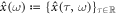 a 4D trajectory of a spin-less electron for ω. Therefore,
  is an existence probability of
  . A stochastic process is non-differentiable, but continuous. Then, the following two vectors are different for a positive dτ:
  and
and  . We remark an inequality
  . Where,
  is decomposed by the following two methods with
  the resolution of them:


It reminds us of idea that  is calculated by the integrals of
  and
and  w.r.t. large enough n. Let us express it by

Recall dx(τ) = v(x(τ))dτ as classical kinematics to draw x. As an analogy of this, we suppose stochastic kinematics as follows:

The first term in RHS of equation (21) shows its drift like classical kinematics.  and
and  are 4D random processes. We set each averages of
  and
and  are zero for all τ:
 ![${\mathbb{E}}[\kern-2pt[ {{dW}}_{\pm }(\tau ,\bullet )]\kern-2pt] =0$](https://content.cld.iop.org/journals/2516-1067/1/2/025011/revision1/prexab1719ieqn90.gif) with
with ![${\mathbb{E}}[\kern-2pt[ f(\bullet )]\kern-2pt] := {\int }_{{\rm{\Omega }}}f(\omega )d{\mathscr{P}}(\omega )$](https://content.cld.iop.org/journals/2516-1067/1/2/025011/revision1/prexab1719ieqn91.gif) an expectation of
an expectation of  wrt
wrt  . Both W± (ω) provide non-differentiability of
  . The randomness
  represents quantum uncertainty of a position of a quanta.
Quantum dynamics is required for the definition of  in equation (21). Recall equation (3) for dx = vdτ. Quantum dynamics has to be the KG equation (17) in the present case. Let us express quantum dynamics of equation (17) by

with operators

as [31] suggests. The form of equation (22) is similar to equation (3). Suppose  and
and

too. Therefore, the drift velocities in equation (21) are given by  . The equivalency between equation (22) and the KG equation (17) is demonstrated by
with an assumption that ϕ is a solution of equation (17) [31].
However when we don't know that ϕ is a solution of equation (17), equation (25) leads  with a free constant C. We need to put an extra rule, C = c2, for the equivalency between equation (17) and equation (22). That is the holonomic constraint in relativistic stochastic mechanics. As [27] proposed, this constraint expressed by

is useful as an analogy of the classical one: v2 = c2. Where, A* denotes the complex conjugate of A. The compatibility between equation (22) and equation (26) will be shown in equation (36) mathematically. We regard the minimum construction of relativistic stochastic mechanics is the triplet of equation (21), equation (22) and equation (26) as quantum mechanics.
3.2. Mathematical remarks
We recall mathematical remarks for equation (21) and equation (26) briefly. A probability measure  for
for  provides
  a distribution of sample trajectories at τ wrt Equation (21). Suppose a probability density

which follows the Fokker-Planck (FP) equation below:

In the classical limit  , equation (28) expresses a classical advection by
 ![${\partial }_{\tau }p(x,\tau )+{\partial }_{\mu }[{v}^{\mu }(x)p(x,\tau )]=0$](https://content.cld.iop.org/journals/2516-1067/1/2/025011/revision1/prexab1719ieqn104.gif) with
with  , i.e.,
  with classical kinematics
  . When we accept the equivalency between stochastic kinematics of equation (21) and the FP equation (28), the conditions
  give the rules of
  in equation (21), respectively1
:
in equation (21), respectively1
:

Hence, p± in equation (29) describe the distributions of the random processes  at τ. Stochastic kinematics of equation (21) is now characterized mathematically.
Let us introduce the following operator:

We can find  from the above. Since p follows the FP equation (28),

This formulae of ± are applied to many transformations in stochastic mechanics. For example when f(x) = x,

The readers may find the expansion of equation (31) bellow:

This is the so-called differential form of Nelson's partial integral formula [25]. The complex version of equation (33) is much more useful. Recall the definitions of  and
and  ,
,

The superposition of equation (33) of '+' and '−' signs gives

When  and
and  in equation (35),
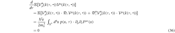
is found by using equation (22). This result bridges between equation (22) and equation (26). This situation is same as the classical one: dv2/dτ = 0 by v2 = c2 and equation (3).
3.3. Ehrenfest's theorem
One of the concerns in quantum mechanics is an expectation of that. Let us consider it in relativistic stochastic mechanics. In order to equation (35), we get


To substitute equation (22) for RHS of equation (38),

This is so-called Ehrenfest's theorem [34] which is an average mechanics of equation (22) as the KG equation (17).
4. Ponderomotive effect in stochastic mechanics
Let us discuss the ponderomotive effect in relativistic stochastic mechanics of a spin-less electron. The KG equation (17) for a slowly varying motion is below: ![${(i{\hslash }\partial )}^{2}\langle \phi \rangle -[{m}_{0}^{2}{c}^{2}-{e}^{2}\langle {A}^{2}\rangle ]\langle \phi \rangle =0$](https://content.cld.iop.org/journals/2516-1067/1/2/025011/revision1/prexab1719ieqn119.gif) . This is an equation which has eliminated the fast oscillation of A in equation (17). This suggests that an effective mass
. This is an equation which has eliminated the fast oscillation of A in equation (17). This suggests that an effective mass  appears in a propagation of a spin-less electron in quantum mechanics. Against this fact, here we confirm the above in stochastic mechanics with the same strategy of one in classical mechanics discussed in section 2. Namely, we will give the strict solution of stochastic mechanics at first, then find an equation of a slowly varying motion. Let us consider dW± (ω) in equation (21) are another types of oscillations from one of A.
In this section, we consider the '+' sign of equation (21). Therefore, the determination of  is our first problem. This is found by
 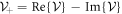 with equation (24). To give
  by equation (24), ϕ a wave function of the KG equation is required. Again suppose a laser field is a plane wave, i.e., A = A(k · x) and let p be an initial 4-momentum of a spin-less electron (
 ). Under this situation, we know the Volkov solution [35] which is an analytic solution of the KG equation (17).

 of equation (24) is calculated strictly as follows:

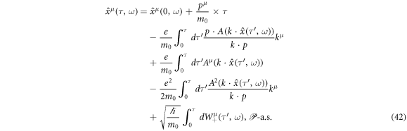
The readers should compare this with equation (4).  is satisfied since
  in our present case. Therefore, equation (41) is a drift velocity of a spin-less electron. We hereby express a trajectory of a spin-less electron in a background laser field of a plane wave by the integral of equation (21) corresponding to equation (5):
Recall the fact that we have to give the three of a holonomic constraint, stochastic kinematics and quantum dynamics of a spin-less electron dressing a laser field in relativistic stochastic mechanics. Let us find that triplet for the ponderomotive effect from the holonomic constraint. Consider the Itô formula of  for the '+' sign of equation (21)2
:
for the '+' sign of equation (21)2
:
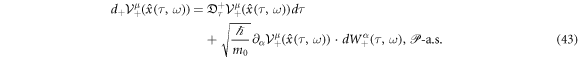
For  since
since  and
and  in the present situation,

is the quantum version of equation (9). Where, 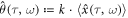 . The operation
  to extract a slowly varying part acts on only A of an external laser field. Conversely, let
  since the random oscillation of W+(ω) is independent from A. The second term of randomness in RHS of equation (44) is the difference from classical mechanics after the operation
  . We can find that
  is parallel to the 4-wave vector k even if there is that random term. A 4-velocity in a slowly varying motion

(use equation (41)) provides the following relation:

Instead of this relation, the readers may find its another expression such as

for a stochastic process  . Again, let us introduce the effective mass

and the effective proper time τeff by

Consider the replacements of variables:  ,
,  and
and
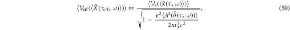
Now the rule of the 4-velocity squared in our model is recovered for all ω:

This is the holonomic constraint of a spin-less electron dressing a plane wave laser field described by the effective variables. This is a special case of equation (26): ![${\mathbb{E}}[\kern-2pt[ \mathrm{LHS}\,\mathrm{of}\,\mathrm{Eq}.(51)]\kern-2pt] ={c}^{2}$](https://content.cld.iop.org/journals/2516-1067/1/2/025011/revision1/prexab1719ieqn143.gif) , too. The plus sign of stochastic kinematics of equation (21) as the second item in stochastic mechanics is replaced by
, too. The plus sign of stochastic kinematics of equation (21) as the second item in stochastic mechanics is replaced by

with  due to equation (29):
  for
for 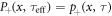 and the fact that meff is a function of
  . Namely, a stochastic trajectory is,

when  . The readers have to confirm the relation below:
 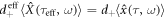 . Define the operator

appearing in the following Itô formula for  by equation (52) with its probability
  :
:

Then, quantum dynamics as the third important element in our model for the ponderomotive effect is

This is derived from 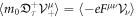 . Equation (56) is equivalent to the KG equation

as we discussed in the first part of this section with


Equation (57) shows that the ponderomotive effect is a free propagation of a spin-less electron dressing an external field. We could formulate quantum dynamics of equation (56) similar to equation (15) in the classical regime. When f in equation (55) is replaced by  ,
,
expresses the time evolution of a momentum 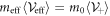 along
along  instead of equation (44). The triplet of equation (51), equation (52) and equation (56) are relativistic stochastic mechanics for the ponderomotive effect acting on a spin-less electron at
  .
.
Consider the FP equation for equation (52):

With  the probability density at τeff for
 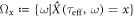 . We can expect peff is a function of k · x and τeff since
  is a vector function of k · x. Then, the RHS of the above equation becomes zero since kμkμ = 0. Therefore, stochastic kinematics of equation (52) imposes the following advection equation of its probability distribution peff:

So, a profile of peff free propagates in the spacetime with the 4-velocity of  . In order to the rule of randomness
 ![${\mathbb{E}}[\kern-2pt[ {{dW}}_{+}^{\alpha }({\tau }_{\mathrm{eff}},\bullet )]\kern-2pt] =0$](https://content.cld.iop.org/journals/2516-1067/1/2/025011/revision1/prexab1719ieqn161.gif) , the expectation of equations (51), (52), (56) gives its Ehrenfest's theorem
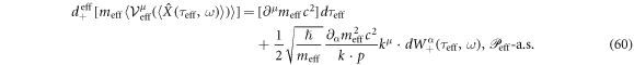
, the expectation of equations (51), (52), (56) gives its Ehrenfest's theorem

and this is comparable with equation (15), too, where we dare to write the index of meff in equation (63) since

in general. It shows a difference between the present model and equation (15) of classical mechanics. A spin-less electron stays in  at τeff. For

a typical radius of a spin-less electron, let re be the Compton wavelength, i.e., re = 6.5 × 10⁻¹²m. A typical pulse duration of a high-intensity laser is the order of 30fsec equivalent to 10μ m and its wavelength is order of 1 μ m [1–6] against the order of re. Hence, the domain  is point-like for
  at τeff. Therefore,

is reasonable for the interactions of a spin-less electron with a high-intensity femtosecond laser field. Then, equation (63) with equation (66) becomes equivalent to equation (15) of classical mechanics. The similarity of formulae between equation (15) and equations (51), (52), (56) shows a universality of a ponderomotive effect acting on a spin-less electron interacting with a high-intensity femtosecond laser field of a plane wave in both classical and quantum regimes.
5. Conclusion
We discussed relativistically covariant formalism of the ponderomotive effect of a spin-less electron interacting with a high-intensity plane wave laser field in classical and in quantum mechanics. The key words in our discussion were, relativistic covariance and a slowly varying component of variables. In section 2, we recalled the relativistically covariant form of the ponderomotive effect in classical mechanics. We derived this by solving equation (3) strictly with a plane wave laser field. Where, the effective mass meff of equation (13) was defined to express a spin-less electron dressing a laser field. Its gradient force  was identified as the relativistically covariant ponderomotive force. To discuss the above in the quantum regime, we introduced relativistic stochastic mechanics in section 3. It was constructed by stochastic kinematics of equation (21), quantum dynamics of equation (22) equivalent to the KG equation (17) and the holonomic constraint of equation (26). By using this in section 4, we expressed the ponderomotive effect in the quantum regime. Namely, the triplet of equations (51), (52), (56) was derived as relativistic stochastic mechanics for the ponderomotive effect. It related with
  the wave function of a slowly varying spin-less electron of its mass meff. Thus, relativistic stochastic mechanics also imposed meff in the ponderomotive effect. Where,
  of equation (53) is a realistic trajectory of a scalar electron. The ability to draw
  by the present model is the unique achievement in quantum mechanics since stochastic kinematics has been absent in usual quantum mechanics so far. For
  ,
,

in equation (60) provided the momentum transfer of a spin-less electron due to the ponderomotive force f. Both classical and quantum dynamics have the term of  . This imposed the universality of the ponderomotive effect bridging between both regimes with a typical high-intensity femtosecond laser of a plane wave. Hence, we concluded relativistic classical mechanics is enough to express the purely ponderomotive effect in laser-plasmas produced by a high-intensity femtosecond laser via equation (66). Let us consider the inequality of equation (64). Equation (66) was derived by the treatment such that
 ![${\mathbb{E}}[\kern-2pt[ {\partial }^{\mu }{m}_{\mathrm{eff}}(\langle \hat{X}({\tau }_{\mathrm{eff}},\bullet )\rangle )]\kern-2pt] $](https://content.cld.iop.org/journals/2516-1067/1/2/025011/revision1/prexab1719ieqn171.gif) was approximated by
was approximated by ![${\partial }^{\mu }{m}_{\mathrm{eff}}({\mathbb{E}}[\kern-2pt[ \langle \hat{X}({\tau }_{\mathrm{eff}},\bullet )\rangle ]\kern-2pt] )$](https://content.cld.iop.org/journals/2516-1067/1/2/025011/revision1/prexab1719ieqn172.gif) since
since  the domain of the probability density of a spin-less electron was point-like for
  of a high-intensity femtosecond laser in equation (63). Therefore, we can find the inequality of equation (64) when
  is not point-like for
  . This inequality expresses quantumness of the a scalar electron dressing a laser field. A possibility to see this may be examined by extremely short pulse lasers like recent attosecond lasers (for example [2]) or forthcoming high-intensity zeptosecond lasers like IZEST project [36].
Finally, KS was impressed by Kibble's work of [22]. He also argued the classical-quantum correspondence in that paper. He explained that by Ehrenfest's theorem like equation (63) in the present article. Then, ![${m}_{0}[{\partial }_{t}{\boldsymbol{v}}+{\boldsymbol{v}}\cdot {\rm{\nabla }}{\boldsymbol{v}}]=-e({\boldsymbol{E}}+{\boldsymbol{v}}\times {\boldsymbol{B}})$](https://content.cld.iop.org/journals/2516-1067/1/2/025011/revision1/prexab1719ieqn177.gif) as equation (50) in [22] was suggested. This is almost same as following Nelson's stochastic mechanics
as equation (50) in [22] was suggested. This is almost same as following Nelson's stochastic mechanics

with  assisted by the Schrödinger equation
 ![$i{\hslash }{\partial }_{t}\psi =1/2{m}_{0}\times {[-i{\hslash }{\rm{\nabla }}+{eA}]}^{2}\psi $](https://content.cld.iop.org/journals/2516-1067/1/2/025011/revision1/prexab1719ieqn179.gif) . This Nelson's model is coupled with a 3D stochastic process given by its kinematics [24, 25]. Our discussion in section 4 for relativistic dynamics
. This Nelson's model is coupled with a 3D stochastic process given by its kinematics [24, 25]. Our discussion in section 4 for relativistic dynamics 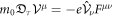 is regarded as the natural expansion of the above non-relativistic dynamics, with stochastic kinematics to illustrate a realistic trajectory of a quanta.
Acknowledgments
KS acknowledges Prof K A Tanaka (ELI-NP), Dr J F Ong (ELI-NP), Dr Y Nakamiya (ELI-NP), Mr J Tamlyn (ELI-NP) and Dr J K Koga (QST, Japan) for useful discussion. This work was supported by the Extreme Light Infrastructure Nuclear Physics (ELI-NP) Phase II, a project co-financed by the Romanian Government and the European Union through the European Regional Development Fund—the Competitiveness Operational Programme (1/07.07.2016, COP, ID 1334).
Footnotes
- 1
The following is the standard way to get equation (29) though we characterize W± by equation (29) in the main body: equation (29) is imposed by the following Itô formulae [32, 33] which are Taylor's expansions for the random processes W± (ω),

with
and . Where, means that a given relation is 'almost surely' satisfied for each ω ∈ Ω. - 2

![${\mathbb{E}}[\kern-2pt[ {{dW}}_{\pm }^{\mu }(\tau ,\bullet )]\kern-2pt] =0$](https://content.cld.iop.org/journals/2516-1067/1/2/025011/revision1/prexab1719ieqn110.gif)
![${\mathbb{E}}[\kern-2pt[ {{dW}}_{\pm }^{\mu }(\tau ,\bullet ){{dW}}_{\pm }^{\nu }(\tau ,\bullet )]\kern-2pt] ={\delta }^{\mu \nu }d\tau $](https://content.cld.iop.org/journals/2516-1067/1/2/025011/revision1/prexab1719ieqn111.gif)


