

Abstract
Operando calorimetry has previously been utilized to study electrochemical reactions and degradation in electrochemical cells such as batteries. Calorimetric data can provide important information on the lifetime and thermal properties of electrochemical cells in practical engineering applications such as thermal management. High temperature electrochemical cells such as solid oxide fuel cells or electrolyzers can also benefit from operando calorimetry, but to the authors' knowledge such capabilities have not been commercially developed. Herein, an operando calorimeter is reported that is capable of simultaneous calorimetry and electrochemistry at temperatures up to 1000 °C and in both oxidizing and reducing atmospheres. The calorimeter is constructed by modifying a commercial apparatus originally designed to study high temperature electrochemical cells in various gas environments. A grey-box, nonlinear system identification model is utilized to analyze both electrochemical and calorimetric data of BaZr0.8Ce0.1Y0.1O3 based electrochemical cells and achieve a calorimeter electrochemical cell power sensitivity of 16.1 ± 11.7 mW. This operando calorimeter provides the capability to study thermal behaviour of electrochemical cells at elevated temperatures.
Export citation and abstract BibTeX RIS
1. Introduction
Operando calorimetry is widely used to study the properties of electrochemical batteries, including the thermodynamics of insertion reactions, phase changes in the active materials, degradation of electrode-active materials during electrochemical cycling, and parasitic side reactions that lower electrochemical cell efficiency [1–3], The decomposition rate of component materials can be used to predict safety events, performance degradation, and overall device lifetime. In addition, the development of thermal models for electrochemical cells as they degrade is useful for thermal management in practical settings [3]. Previously, such studies have primarily focused on the characterization of electrochemical cells operating at or near room temperature. For several reasons, extending operando calorimetry to higher temperatures, and in both oxidizing or reducing atmosphere, can provide valuable diagnostics of electrochemical devices. Fuel cells that operate in the 200 °C–800 °C range under exposure to both highly reducing (H2) and highly oxidizing (O2) atmosphere are widely studied as a promising technology [4, 5]. There is also growing interest in high temperature solid oxide electrolysis and CO2 reduction to synthetic fuels [6, 7]. In these systems, calorimetry can provide direct, independent characterization of gas phase reactions aside from that which is inferred from electrical measurements, given each half-cell reaction has an associated enthalpy and entropy. Importantly, calorimetric measurements can shed light on side reactions, including those associated with solid electrolyte degradation, which are of utmost importance to both efficiency and life [5]. While some previous studies have used thermal techniques such as differential scanning calorimetry to determine temperature stability windows and rates of degradation in solid electrolytes [8–11], these methods have been performed ex situ rather than during the operation of devices, which may present entirely different conditions affecting electrolyte stability. Other failure modes such as mechanical failures allowing direction reaction of the fuel and oxidant are typically difficult to detect from electrical measurements alone (until the failure is catastrophic), but could be detected thermally. Solid-state phase transformations occurring in components of the electrochemical cell as a function of temperature and thermal history are another category of phenomena that can be measured thermally via calorimetry, but are difficult to detect and quantify electrically.
High temperature calorimeters are common but typically operate in the differential scanning calorimetry mode [12, 13], which is not amenable to simultaneous application of multiple reactive gas streams and electrochemistry. Therefore, it is not surprising that calorimeters with the desired capabilities have not previously been reported in the literature and are not available commercially. To build such a calorimeter is not straightforward. The materials required to construct the necessary calorimeter components, such as the calorimeter housing or vessel, the temperature probes, and the electrical connections, are subject to attack by both H2 and O2, as well as by any water vapour present. Furthermore, the different gas streams in a fuel cell must be well-separated to avert safety issues resulting from mixing at high temperature.
Herein, a calorimeter capable of operando measurements of high temperature electrochemical cells under oxidizing or reducing gas environments (or both simultaneously) is described. Extensive modifications were performed on a commercially available apparatus, the ProboStatTM (Norwegian Electro Ceramics AS), to enable operando calorimetry. By using an apparatus developed for the study of electrochemical cells such as fuel cells at high temperatures in various gas ambients, the baseline performance was well established, and efforts could be focused on developing the calorimetric capability. By retaining the original furnace configuration, and adding minimal new thermal mass, the original heating and cooling rate capabilities of the instrument were also retained. The maximum ramp rates are 25–35 C min−1, depending on the temperature and the gas flow rate in the usual way. It is shown that the apparatus developed here enables simultaneous extraction of thermodynamic and kinetic parameters upon combining electrochemical and calorimetric techniques. Examples from calorimetric and electrochemical testing of BaZr0.8Ce0.1Y0.1O3 (BZCY) electrolyte-based electrochemical cells are presented.
2. Experimental
2.1. Design objectives
The calorimeter's temperature, atmosphere, and electrochemistry capabilities presented here are designed to support operando studies of high temperature solid electrolytes. The target range of values for the key performance parameters are presented in table 1. The operating temperature range, from room temperature to 1000 °C, includes the typical temperature range of interest for solid oxide fuel cells (SOFCs). The electrical parameters allow for the application of electrochemistry and the use of temperature sensors for the calorimeter. With at least two temperature probes, each utilizing two connections, and a two-electrode setup to probe the electrochemical cell or device, a minimum of six electrical connections are needed. If additional capabilities are needed, such as three-electrode electrochemical cells or four-point-probe electrical measurements, up to 11 electrical connections may be required. Designing the calorimeter to enable the use of two different gases simultaneously is necessary for testing fuel cells under realistic operating conditions. The samples used have a diameter of approximately 20 mm, a common size format in literature [8, 10].
Table 1. Calorimeter design objectives for the study of high temperature solid electrolytes.
| Specification | Minimum value | Maximum value |
|---|---|---|
| Temperature | 20 °C | 1000 °C |
| Voltage | −20 V | 20 V |
| Current | 0 mA | 400 mA |
| Electrical connections | 6 | 11 |
| Number of gases | 1 | 2 |
| Sample diameter | 10 mm | 30 mm |
| Sensitivity | <50 mW |
A typical target for electrical power density in fuel cells is 500–2000 mW cm−2 [14]. Because currently fuel cells are approximately 50% efficient [15], a 500 mW cm−2 thermal power density is assumed here, representing the low end of the above range. The goal of the present calorimeter design is to capture at least 10% of that power. Therefore, the minimum sensitivity is 50 mW, assuming a minimum active electrode area of 1 cm2. Furthermore, estimates from solid oxide electrolyte side reactions in the literature [10] show heat effects of order 100 mW g−1. Assuming that samples contain 1 g of material, typical for the sample dimensions used here, heat effects are expected to be on the order of 100 mW for these reactions, which is measurable at the target sensitivity.
2.2. Calorimeter design
The calorimeter presented here modifies a commercially available high temperature electrochemistry apparatus, the ProboStatTM (figures 1 and A1), which provides the necessary temperature range, electrical connections to power the fuel cell samples and temperature sensors, and two-gas capability. The apparatus tubing is made from either alumina for high temperatures (>600 °C) or quartz for medium temperatures (<600 °C), and the section exposed to elevated temperatures uses electrical connections made from platinum. Both materials remain inert and structurally stable in high temperature H2 and O2 ambient. Here the ProboStatTM is operated within a vertically mounted 18" tube furnace (Mellen) that can reach temperatures in excess of 1000 °C.
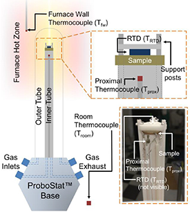
Figure 1. Schematic of a calorimeter, based off a ProboStatTM high temperature electrochemistry apparatus, for calorimetry of high temperature solid state proton conductors. A sample is mounted into the ProboStatTM, which is placed in a vertical tube furnace. The apparatus is modified with several thermocouples to detect local furnace temperature (Tfw ), the temperature proximal to the sample (Tprox ), and the surrounding room temperature (Troom ).
Download figure:
Standard image High-resolution imageModifications to the ProboStatTM are made through the addition and relocation of temperature sensors. An S-type thermocouple that is provided with the ProboStatTM for monitoring the approximate sample temperature is relocated to the alumina support post below the sample and cemented (Cotronics Resbond 907GF, a high temperature cement) in place for better heat conduction. This thermocouple is used to measure the temperature proximal to the location of the sample (Tprox ). A small, thin film resistance temperature detector (RTD, Omega F3142 or US Sensor PPG102A1) is attached to the sample itself, using the same high temperature cement. In addition to the furnace thermocouple used by its proportional-integral-derivative (PID) temperature controller, a K-type thermocouple (Tfw ) is attached to the wall of the furnace near the sample. Tfw is used to acquire a more accurate temperature reading of the furnace temperature, picking up fluctuations in the wall temperature that are not recorded by the PID thermocouple. Finally the temperature of the room is monitored using a K-type thermocouple (Troom ) located in the vicinity of the ProboStatTM base. All temperature data from thermocouples are recorded using an eight channel data acquisition module (Omega).
The electrical connection schematic is shown in figure 2(a). The ProboStatTM is designed for a maximum of six electrical connections for power applications and up to six thermocouple connections. One pair of thermocouple connections is used for Tprox . All six power connections are used. Two of these electrical connections are used for operating the RTD, while four are connected to the sample. Two connections are made to opposite ends of the cathode to enable current flow across the cathode, as discussed in section 4.1, in order to simulate heat-generating reactions at the electrolyte-electrode interface. In addition, one connection is made to the anode, and another is made to the reference electrode of the sample. In certain cases, additional connections are needed for four-point measurements or other types of electrical stimulation or monitoring. In those situations, voltage measurements can be made using the unused thermocouple connections, while reserving the other electrical connections for running current. All electrical sourcing and measurement is performed using a commercial potentiostat (Bio-Logic).

Figure 2. (a) Electrical diagram for the calorimeter. The ProboStatTM Base Connections correspond to connection ports labelled in the corresponding manner on the apparatus and are connected to various components of the setup. Two connections are made to a resistance temperature detector (RTD). Four connections are made to the sample: two to the cathode (Cat+ and Cat−), one to the anode (An), and one to the reference (Ref). Two connections are made to a thermocouple proximal to the sample (Tprox ). (b) Fluidic diagram of the calorimeter. Two gas streams flow into the outer tube volume and the inner tube volume of the calorimeter. The sample can be sealed to separate the two gases if they are different. Two bubblers are placed in line to allow for humidified gas.
Download figure:
Standard image High-resolution imageThe calorimeter's fluidic infrastructure is designed for use of up to two gases with the option of running those gases dry or humidified (figure 2(b)). The sample, sealed to the inner tube of the ProboStatTM, serves to isolate the gases and prevent mixing. A water bubbler is used to humidify gases at room temperature to about 3% (0.03 atm). The gases are flowed through the ProboStatTM at flow rates typically between 5–20 ml min−1.
The calorimeter can support samples between 10 and 30 mm in diameter and between 0.5 and 10 mm in thickness, which corresponds to a sample mass of up to approximately 10 g. These samples are mounted into the ProbostatTM with the appropriate electrical connections and can be sealed to the inner tube to allow for the simultaneous use of two gas atmospheres, each being exposed to one side of the sample.
2.3. Sample design
In order to test the high temperature performance of the calorimeter, cells in the configuration of an electrochemical hydrogen pump using BZCY as the solid proton conductor were used. This cell is simpler than the corresponding high temperature fuel cell since H2 is supplied to both sides of the sample; a fully operational fuel cell results if H2 and O2 are supplied to the anode and cathode respectively. Operating as a hydrogen pump, hydrogen gas is oxidized at the anode, supplying protons which diffuse through the solid electrolyte to the cathode whereupon they are reduced and evolve hydrogen gas. No net molecules of hydrogen are produced or consumed in this operation, but since ionic current does flow through the electrolyte, it mimics the electrochemical operation of a solid oxide fuel cell.
The sample was constructed using a 20 mm diameter and 1 mm thick BZCY ceramic plate (CoorsTek Membrane Sciences AS) as a platform (figure 3). Thin film Pt and Pd electrodes are used as catalysts to promote the H evolution and oxidation reactions at the surfaces of the BZCY disk. A cathode, anode, and reference electrode each between 20 and200 nm thick were sputtered on top of a 3–4 nm thick sputtered Cr adhesion layer, using Kapton tape to mask off areas between the electrodes. To monitor the local temperature an RTD (Omega F3142 or US Sensor PPG102A1) was cemented on top of the cathode side of the sample, making sure that the RTD leads do not short to the cathode surface. The RTDs used in this report have a maximum operating temperature of 600 °C. However, RTD's with higher maximum operating temperatures are available (US Sensor PPG201B3 and PPG201E7) for studies at higher temperatures.

Figure 3. (a) Schematic of sample with mounted resistance temperature detector (RTD). The sample contains a 20–200 nm Pd or Pt thin film cathode separated from a 20–200 nm Pd or Pt thin film anode and a ring-shaped reference by a 20 mm diameter and 1 mm thick BZCY ceramic electrolyte. 3–4 nm of Cr is used as an adhesion layer between the metal electrodes and ceramic electrolyte. (b) Photos of the top and bottom of the sample.
Download figure:
Standard image High-resolution image3. Results
3.1. Inferring heat flow with a nonlinear lumped-parameter model
A nonlinear lumped-parameter model is used to describe the behaviour of heat transfer within the calorimeter, similar to the method of MacLeod et al [16]. The dynamics of this system are approximated using a grey-box approach. This entails developing an appropriate equivalent circuit model to describe the heat flow pathways through the calorimeter, and then experimentally obtaining the parameters of the model through a calibration process. The model is calibrated by measuring temperature changes at various temperature probes that result from input power of known quantities. The relationship between power and temperature in the model is thus established. The calibrated model allows the output power to be predicted knowing only the input power and temperatures of those temperature probes. Any mismatch between the input and output powers can then be attributed to thermal events in the cell, e.g. side reactions or degradation, which along with electrochemical data can be analyzed to gain insight on the performance of the cell and its components over time.
3.2. Nonlinear equivalent circuit model of the calorimeter
A one-state, nonlinear equivalent circuit diagram of the calorimeter is shown in figure 4(a). Numerous model candidates were analyzed, including two- and three-state models, but this one-state model with two nodes and three measured grounds was determined to be the model that provides the best calorimeter sensitivity.
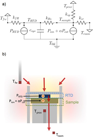
Figure 4. (a) Equivalent circuit diagram of the calorimeter. The model consists of two nodes represented by TRTD and Tsample but just one state capacitor csys for the system. There are three signal grounds represented by the furnace temperature Tfw , the proximal thermocouple temperature Tprox , and room temperature Troom . One additional absolute ground T0K is used as a reference for heat capacitance. Powers from three different sources located at or near the sample are presented by PRTD, Pion , and Pcat . See text for explanation of other symbols. (b) Physical model of heat flow within the calorimeter. Red arrows indicate the direction of heat flow starting from the furnace hot zone to the outside environment. Physical approximations of the nodes corresponding to TRTD and Tsample , as well as PRTD, Pion , and Pcat labelled in (a) are also shown.
Download figure:
Standard image High-resolution imageIn this equivalent circuit model, the resistors represent heat conductances between different nodes. A capacitor represents a heat capacitance, while grounds represent thermal sources and sinks. Power inputs are modelled as current sources. The model has one measured node, TRTD , and one unmeasured node, Tsample , although only one heat capacitance is needed to approximate both. Other than the absolute ground used to reference power inputs and heat capacitance, there are three grounds in this model: one source and two sinks.
Figure 4(b) shows the heat flow pathways in the system in relation to a schematic representation of the sample, supports, and temperature sensors. This diagram illustrates the physical origins of the heat flows within the system that are represented in the equivalent circuit diagram (figure 4(a)). Heat is generated in the furnace, represented by Tfw , and flows to the RTD node, which has a temperature TRTD . Heat then continues to flow through the sample node, an unmeasured node that approximates the sample itself, before exiting out either through an intermediate ground Tprox or the room temperature ground Troom . The need for two sinks stems from the inability of Tprox to capture all of the heat flowing out from the sample node due to other heat flow pathways out to the surrounding environment.
The model includes three power sources that correspond to the different power inputs to the sample during either calibration or testing. PRTD is a baseline power that is emitted by the RTD when in operation. Typically for a 1 kΩ RTD a sense current of 1 mA is used, generating between 1 and 5 mW of power, depending on the temperature of the system. Pion is the power generated from operating the solid electrochemical cell. It is caused by both resistive heating of the solid electrolyte and reaction overpotential losses. Lastly, Pcat is used to study surface reactions or other surface phenomena related to the solid electrolyte. This power is approximated during calibration of the model by running current laterally across the cathode of the sample. Two nodes were modelled to appropriately capture system dynamics. The time constant for heat detection by the RTD for a heat source originating within the RTD (PRTD ) is smaller than the time constant for heat detection when the source is nearby, but not within, the RTD itself (Pion and Pcat ).
The dynamics of the system described by the equivalent circuit diagram can be distilled into the following system of equations, in which cx are capacitances, kxx are conductances, and α is a scale factor fitted to adjust Pcat based on the ratio of Pcat:Pion detected by the temperature probes in the calorimeter:


where


Although equations (1) and (2) could be combined into one equation, thereby eliminating Tsample , they are split out to better represent the physical model. Each element in the model is split out to second order nonlinear parameters, which aggregates to 18 possible parameters to be fitted. For operation within a limited temperature range, the model typically does not need to be fit with second order nonlinear parameters, so just zeroth and sometimes first order parameters can be used.
3.3. Experimental calibration of operando calorimeter
The operation of the operando calorimeter in a test case where the sample is a thin disc of a BZCY proton conductor, coated with sputtered Pt electrodes on both faces, is now demonstrated. The instrument was first used to measure the conductivity of the BZCY solid electrolyte, and yielded expected results over the temperature range from 350 to 850 °C in 4% humidified H2 in Ar (figure 5, and appendix

Figure 5. Conductivity of a BaZr0.8Ce0.1Y0.1O3 (BZCY) solid electrolyte, measured in the operando calorimeter in humidified 4% H2 in Ar. The calorimeter was then tested with this test sample in place.
Download figure:
Standard image High-resolution imageNext, the calorimeter was calibrated by establishing a set of parameters for the model that produce an output matching experimental results. Three sources of input power, PRTD, Pcat , and Pion , representing three possible sources of heat generated during an experiment, were supplied. Each as a different temporal variation, as shown in figure 6(a). The largest temporal variation in input power was for Pion , the power supplied to the solid electrolyte, as would be the case during actual operation of the device as an electrochemical cell. Three of the corresponding temperature measurements are shown in figure 6(b). Tfw, Tprox , and Troom (not shown) are the grounds in the model, see figure 4(a). TRTD,meas is the measured temperature at the RTD node, TRTD in the model in figure 4(a). The input power from figure 4(a) and temperatures in figure 4(b) were then analyzed with a MATLAB script utilizing the MATLAB System Identification ToolboxTM nlgreyest procedure, similar to one described by MacLeod et al [16, 17]. The script takes the model described by equations (1)–(8), as well as the input power and ground temperatures, and estimates the vector of model parameters θ to create a modelled version of TRTD , here referred to as TRTD,mod . A search for fitted model parameters is initiated and iterated in order to minimize a cost function


Figure 6. A calibration run performed on a Pd thin film coated BZCY sample at elevated temperatures in humidified H2 gas for determining model parameters. (a) Calibration input powers from three input sources, (b) temperature outputs, and (c) a fit between the modelled temperature and the measured one. The normalized root mean square error (NRMSE) of the fit is 79%. (d)–(f) are expanded views of sections of (a)–(c) that show fine scale details of the signals.
Download figure:
Standard image High-resolution imagewhere t is the discretized time of each datapoint in the dataset ranging from 0 to tmax . A differential measurement between either the measured or the modelled temperature at the RTD node and a nearby temperature ground allows for fits to be made on smaller temperature ranges, and cancels out the majority of noise coming from the furnace, improving the goodness of fit. Typically only linear (zeroth order) terms for each element in the model are initially fitted, in order to scan for a global minimum in V(θ) with lower computational effort. Upon approaching a perceived cost function minimum, first order, nonlinear terms for each circuit element are then allowed to vary as well. It was found that second order, nonlinear terms are rarely necessary unless the experiment spans a temperature range of over several 100 °C.
After a suitable search and refinement of the model parameters θ that minimizes V(θ) below a certain cost tolerance, θ is considered to have reached at least a locally minimized value, θminimized
. Upon reaching V(θminimized
), the measurement, ΔTmeas
, is compared to the model, ΔTmod
, as illustrated in figure 4(c). An example of a parameter set for θminimized
are shown in table A1 of appendix
3.4. Determining calorimeter sensitivity
To verify that the fitted model is applicable to a wide variety of datasets, and not just the one used for calibration, a second series of experiments was conducted. A set of input power signals utilizing different waveforms and magnitudes was used. The input powers from part of such a run are highlighted in figure 7(a), along with temperature in figure 7(b). Using the parameter set, θminimized
, from the previous experiment, TRTD,meas
was used to in conjunction with the measured temperature grounds to recover a model of the input power. This modelled power can then be compared with the original input power to see how well the model reconstructs the power data (figure 7(c)). The residual power is calculated as the difference between these two powers (figure 7(d)). The standard deviation of the residual power is a measure of the calorimeter's lower limit of detection. However, an adjustment needs to be made to account for the fact that power is measured at the RTD node in the model while the input powers of interest (Pion
and Pcat
) originate at the sample node. Since only a fraction of the sample node's power flows into the RTD node, the power signal as well as the noise in the power are dampened. To correct for this effect, the standard deviation is multiplied by an adjustment factor from a node-to-node heat flow analysis described in appendix
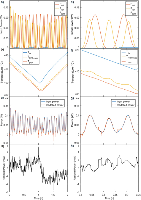
Figure 7. Arbitrary power inputs applied with a BZCY sample in place at elevated temperatures in humidified H2 gas are used to verify calibration parameters and determine the calorimeter sensitivity. (a) Input powers from three sources of different waveforms, (b) temperature outputs, (c) a fit between the modelled power and measured one, and (d) the residual power taken from the difference between the input and modelled powers. The standard deviation of the residual power (1.7 mW in this case) is used to determine the calorimeter sensitivity. (e)–(h) are expanded views of (a)–(d) showing finer-scale details of the signals.
Download figure:
Standard image High-resolution image3.5. Operando calorimetry of the BZCY-based electrochemical cells
The above-described sequence of experiments was repeated seven times, once after each BZCY sample was loaded into the electrochemical cell and brought to operating temperature in H2 atmosphere, and produced the results shown in figure 8. The calorimeter was found to have an average sensitivity of 16.1 ± 11.7 mW throughout these experiments, which exceeded the initial design objective of 50 mW sensitivity. The performance of the calorimeter did vary somewhat between the seven experiments, which could be due to some differences in sample preparation and mounting in the calorimeter.
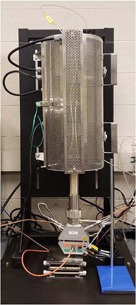
Figure 8. Calorimeter sensitivity and average power residuals obtained for runs with seven BZCY samples. Calorimeter sensitivity is defined as the adjusted residual power level above which heat unexplained by known input powers is observed. The average calorimeter sensitivity is 16.1 ± 11.7 mW. In all seven runs, the average power residual is well within the sensitivity for that run, showing an absence of detectable heat-producing reactions.
Download figure:
Standard image High-resolution imageThe average power residuals plotted in figure 8 are the time average of all the power residuals measured during a run such as in figure 7. The fact that these power residuals are well below the sensitivity of the calorimeter for each of the samples demonstrates that the parameter set θminimized determined during calibration is able to model the response of the system over the range of input power used and the corresponding temperature fluctuations. For the simple BZCY hydrogen pump tested here, no excess power was detected that could not be accounted for by the electrical inputs to the electrochemical cell, indicating that within the sensitivity of the operando calorimeter, no heat-producing degradation or side reactions were detected.
4. Future improvements
The instruments and analytical methods described here represent the first operando calorimeter of which the authors are aware that can perform measurements with 10–20 mW sensitivity under the challenging conditions of elevated temperature, varying gas environments, and simultaneous electrochemical measurements. While commercial calorimeters optimized for sensitivity can detect on the order of 10–100 µW, they have maximum temperatures limited to ~100 °C and are not capable of simultaneous electrochemistry. Certain modifications can be made to improve the resolution of the present instrument. Perhaps the biggest shortcoming is that the RTD mounted on the sample is not able to capture more of the heat generated at the sample. Minimizing thermal conduction from the sample to the furnace wall and the room temperature ground would help in this regard, for example by using thinner alumina for tubing and supports in contact with the sample, or introducing a thermal insulator (e.g. an aerogel) between the sample and the support tube. Using thinner measurement wires to the sample could also help.
Substantial gains in sensitivity could be achieved by improving sensing of heat flow from the sample. The current design has a single proximal thermocouple Tprox subtending only part of the alumina tube extending from the sample. Introducing more thermocouples, or adding thermally conductive materials in the appropriate location, would allow a larger percentage of the heat emitted from the sample to be measured, as well as smoothing any spatial inhomogeneities in heat production. Run-to-run reproducibility could be improved by reducing the spatial freedom currently available for sample positioning.
5. Conclusions
A calorimeter has been presented here to study operando high temperature solid state electrochemistry, namely solid electrolytes for fuel cells and other similar applications. It can operate between room temperature and 1000 °C and can support up to 12 electrical and thermocouple connections, as well as expose samples to two different gas environments. The calorimeter has a sensitivity of 16.1 ± 11.7 mW and can be constructed from a commercial apparatus and temperature sensors. The capabilities of the calorimeter were demonstrated on BaZr0.8Ce0.1Y0.1O3 based solid electrochemical cells at 400 °C, which showed no thermal degradation of the cell.
Additionally, a heat transfer equivalent circuit model and grey-box system identification technique has been described that allows for the estimation of system parameters and reproducible analysis of experimental data. This technique gives flexibility to the modification of both sample and apparatus design. In most circumstances, only model parameters are changed, and, in the worst case, the model is modified to include additional dynamics to the system, though the overall procedure for data analysis remains the same.
This calorimetry system provides the means to directly study the thermal characteristics and dynamics of solid electrolytes operando. These findings, when coupled with electrochemical data, can provide insights into electrochemical cell performance such as efficiency or power degradation, device life, and cell heating.
Acknowledgments
We thank Matt Trevithick and Dr. Ross Koningstein for helpful discussions. Financial support was provided by Google LLC. David Young was supported by the National Science Foundation Graduate Research Fellowship under Grant No. 1122374.
Appendix A.: Calorimeter and its equivalent circuit model parameters

Figure A1. The ProboStatTM calorimeter setup inside a vertically mounted furnace and accompanying gas and electrical hookups.
Download figure:
Standard image High-resolution imageTable A1. Fitted parameters a obtained from a calibration utilizing MATLAB's nlgreyest function to fit calibration input powers and measured temperatures to a calorimeter equivalent circuit model.
| Parameter | Calibration value | Uncertainty |
|---|---|---|
| csys ,0 | 2.19 × 10⁻¹ J K−1 | 6.2% |
| kRs ,0 | 1.31 × 10⁻² W K−1 | 4.9% |
| kfR ,0 | 4.84 × 10⁻³ W K−1 | 4.6% |
| kfR ,1 | −5.42 × 10⁻⁶ W K−2 | 5.1% |
| ksp ,0 | 7.11 × 10⁻² W K−1 | 1.0% |
| α | 3.10E-1 | 2.9% |
a Parameters not included here were not used (i.e. value of zero) in this model fitting.
Appendix B.: Determination of the adjustment factor used to derive calorimeter sensitivity
During calibration and prediction steps that determine calorimeter model parameters and calorimeter sensitivity, a direct analysis is made on the prediction power residuals to determine their standard deviation. This process is valid, but the resulting magnitude of the residual standard deviation assumes that 1 mW of any input power is equivalent to 1 mW of output power detected by the model. However, in reality, the sensitivity of the model to the ionic power is not the same as its sensitivity to the RTD power because the ionic power is introduced to the model at a different node. By the time the power from the sample node reaches the RTD node, the measured node, it has been dampened by the conductances in the model. In other words, not all power from the sample node flows into the RTD node, so an adjustment factor needs to be created to ascertain the true power sensitivity to the power generated in the sample node. These powers happen to be the ones of interest.
To assess this sensitivity, a calibration or prediction run is reanalyzed, keeping the same fitted parameters and input powers as before, except that the input ionic power is constrained to be 0 for the analysis. The result is shown in figure B1. Because the model does not pick up any ionic power, almost all of the power residuals that appear are due to the ionic power. By measuring the peaks of the residuals and corresponding those to the actual input power, a relative power sensitivity can be obtained. For example, a peak of 25 mW in figure B1(b) corresponds to a known input power of 170 mW in figure B1(a), which suggests that only 15% of the ionic power is collected by the RTD at the RTD node of the model (called the collection factor). Because the sensitivity is determined by the standard deviation of the power residuals, an adjustment factor is calculated using the following equation:


Figure B1. Comparison between (a) the ionic input power and (b) the power residuals observed from running a model fit and setting that ionic input power to zero, while keeping all other parameters, measured temperatures, and input powers the same. From this comparison, a collection factor of 15% is calculated, suggesting that only 15% of the ionic power is detected by the model's temperature measurements.
Download figure:
Standard image High-resolution imageIn this case, the adjustment factor is 2.6. Therefore, a 1.7 mW sensitivity displayed in the model is actually a 4.4 mW sensitivity to the ionic power.
Appendix C.: Verification of electrochemical operation at elevated temperature
Several preliminary studies were performed on testing the operation of BZCY samples to demonstrate various electrochemical capabilities of this system for studying fuel cells. For example, the voltage response to applied current at a range of temperatures is shown in figure C1, demonstrating electrochemistry capabilities of the apparatus up to at least 800 °C.

Figure C1. Demonstration of sustained high temperature electrochemistry in the calorimeter. Current is applied at temperatures between 500 °C and 800 °C in humidified 4% H2. The observed voltage is primarily due to ohmic resistance in the BZCY electrolyte, explaining why the magnitude of voltage decreases with increasing temperature.
Download figure:
Standard image High-resolution image
From these types of initial performance verification studies, the voltage noise resolution is determined to be within 2 mV. Temperature variation on the furnace wall is less than 0.2 °C (standard deviation) at a fixed PID temperature controller set point of 400 °C over ~11 h. However, an offset in the temperature control of the furnace is apparent. The temperature measured by Tfw can be off by as much as +20 °C–40 °C when compared to the furnace set point temperature when operating at high temperatures. Therefore, Tfw is used as the actual temperature of the furnace for the purposes of performing calorimetry.