


Abstract
Despite recent achievements in the design and manufacture of advanced materials, the contributions from first-principles modeling and simulation have remained limited, especially in regards to characterizing how macroscopic properties depend on the heterogeneous microstructure. An improved ability to model and understand these multiscale and anisotropic effects will be critical in designing future materials, especially given rapid improvements in the enabling technologies of additive manufacturing and active metamaterials. In this review, we discuss recent progress in the data-driven modeling of dynamical systems using machine learning and sparse optimization to generate parsimonious macroscopic models that are generalizable and interpretable. Such improvements in model discovery will facilitate the design and characterization of advanced materials by improving efforts in (1) molecular dynamics, (2) obtaining macroscopic constitutive equations, and (3) optimization and control of metamaterials.
Export citation and abstract BibTeX RIS
1. Introduction
Throughout human civilization, materials have quite literally shaped the world we live in. The progression from stone to bronze and iron, and eventually to advanced alloys, has had an unparalleled impact on our technological advancements. The past several decades especially have seen unprecedented progress in material designs [1, 2], including semiconductors, plastics, ceramics, composites, and active materials. These advanced materials have driven nearly every major trillion dollar industry, including energy, health, defense, food and agriculture, construction, manufacturing, transportation, and telecommunications. Of particular recent interest are heterogeneous, multiscale, and anisotropic materials that are able to simultaneously satisfy multiple previously unattainable objectives. It is clear that any science fiction future we envision will be fundamentally enabled by the continued design of tailor-made materials with increasingly exotic, high-performance properties.
Despite rapid progress in the design and production of advanced materials, there is remarkably little first-principles knowledge about the macroscopic behavior of these materials as a function of their microstructure. Although heterogeneity is known to be a key enabling principle in the design of advanced materials, the bulk of theoretical knowledge is centered around modeling linear physics (e.g. acoustics, electromagnetics, linear elastics, etc) for either highly structured heterogeneity (e.g. laminates) or completely random heterogeneity [3]. However, advances in additive manufacturing [4, 5] and meta materials [6–10] are making it possible to design and manufacture increasingly exotic multiscale and anisotropic heterogeneities. Many of these designs are inspired by the incredible properties of biological materials [8, 11, 12]. However, designing the microstructure required to achieve a desired macroscopic set of properties is often intractable, due to the multiple optimization objectives, the high-dimensional and multiscale optimization space, the presence of nonlinear, stochastic, and multi-physics interactions, and the lack of governing equations for the macroscale behavior. Fortunately, machine learning is an emerging field that provides high-dimensional, nonlinear applied optimization based on data that can be tailored to material science discovery.
There are several impressive recent demonstrations of machine learning in materials design and optimization, including for designing superalloys [13, 14] and composites [15], and for the imputation [16] and optimization [17] of macroscopic material properties from constituent compositions and processes. For example, figure 1 shows an example superalloy that was developed using a neural network architecture [13], which identified an advanced material with significantly improved properties and a much more complex composition and process than previous alloys. However, each step of the design optimization may involve a combination of multi-fidelity simulations and experiments, which are extremely expensive in terms of both time and cost. Thus, data-driven learning architectures must operate in the sparse sample limit, with significant missing data and latent variables, which is in direct contrast to the emerging deep learning perspective, where tens of thousands of labeled examples are available. In addition, it is essential to respect known physical constraints and maximally leverage partially known dynamics.

Figure 1. (Left) Advanced super alloy developed using a neural network (reprinted from [13], with the permission of AIP Publishing). (Right) Cement with heterogeneous pebbles. The extreme performance of the advanced super alloy may be thought of in terms of stress distribution in concrete, with stress lines terminating at the pebbles.
Download figure:
Standard image High-resolution imageMore broadly, machine learning is now being used in every field of science, biology and engineering. Much of the earliest efforts in machine learning (often called statistical learning and pattern analysis) was focused on finding patterns in data which could be used for clustering and classification. The field has been well developed, with many books explaining various aspects of the successful methodologies used for these tasks [18–25]. A nice summary of the dominant (top 10) methods of the last decade was also produced by the community in 2008 [26]. In this decade, the community has moved on to deep learning (neural network) architectures due to the abundance of exceptionally large, labeled data sets [27–32]. Deep learning has dominated applications like computer vision, speech and autonomous vehicles. However, deep learning is well known to be difficult to interpret and unable to generalize, thus making is difficult to use in many scientific applications. Only recently has there been a directed effort towards building parsimonious models which attempt to address physical systems which are interpretable and generalizable [33], which is the focus of this review.
1.1. Our perspective: data-driven modeling of multiscale dynamical systems
Model discovery remains a major challenge in the study of materials and their dynamical properties. The goal is to turn data into models that are both predictive and provide insight into the nature of the underlying micro- to macro-scale dynamics that generated the data. Indeed, this problem is made exceptionally difficult by the fact that many systems of interest exhibit diverse behaviors across multiple temporal and spatial scales, all of which are coupled in a typically nontrivial and unknown manner. First principles atomistic and molecular simulations aid in characterizing materials, but often require computationally intractable computations to accurately characterize the coarse-grained, macroscopic scale dynamics. To address these computational and theoretical challenges, we highlight a range of data-driven approaches for discovering nonlinear multiscale dynamical systems from data. These emerging model discovery architectures are well suited for the coarse graining required to characterize material properties. Additionally, we show how these data-driven strategies can be integrated with control protocols in order to manipulate active materials at the macroscopic scale of interest for engineering practice.
We consider two cases of model discovery, (i) when we have access to full measurements, and (ii) and when we have incomplete measurements of the system. When full-state measurements are available, the sparse identification of nonlinear dynamical systems (SINDy) algorithm [34] may be used to discover governing equations. SINDy models are parsimonious, thus they have minimal parametrization, which allows more easily for generalizability and interpretability. When only partial measurements are available, it is possible to use time-delay coordinates to obtain a linear model for the dynamics, via the Hankel alternative view of Koopman (HAVOK) method [35], which is related to dynamic mode decomposition (DMD). These approaches comprise a suite of strategies to discover models for nonlinear multiscale systems.
The machine learning methods proposed here are a significant departure from molecular dynamics (MD) simulations and recently advocated neural network architectures [36–38], for materials modeling. While we are typically interested in macroscopic phenomena, microscale dynamics must also be considered, as they play an important role in driving macroscopic behavior. The macroscale dynamics, in turn, drive the microscale dynamics, thus coupling the dynamics at mulitple scales. This coupling can make multiscale systems particularly challenging, motivating a principled approach to disambiguate the time and spatial scales for model discovery in multiscale systems. The presented methods also circumvent the enormous data requirements required for training deep neural networks, resulting in models that are interpretable and generalizable by design.
The paper is outlined as follows: section 2 introduces a diverse set of data-driven methods and algorithms that will be used in the model discovery framework. Section 3 highlights the modifications and extensions that must be made to these methods in order to accommodate multiscale physics. The integration of data-driven techniques is demonstrated on two problems in section 4: MD simulations and the control of a metamaterials antenna. We conclude in section 5 with an overview of the techniques and commentary on their overall prospectus.
2. Model discovery methods
In this section, we highlight some recently developed model discovery methods that can be modified for applications in multiscale physics. Three mathematical techniques are explored: (i) SINDy, (ii) DMD, and (iii) HAVOK. Each method has an appropriate application depending upon the quality, quantity and observability of the underlying variables. These methods identify dynamical systems to explain spatiotemporal patterns observed in the data.
2.1. SINDy: Sparse identification of nonlinear dynamics
The first highlighted model discovery technique is based upon sparse regression. SINDy [34] bypasses the intractable combinatorial search through all possible model structures, leveraging the fact that many dynamical systems

have dynamics f( · ) with only a few active terms in the space of possible right-hand side functions; for example, the Lorenz equations (see figure 2) only have a few linear and quadratic interaction terms per equation. Here,  is a low-dimensional state, for example obtained via the singular value decomposition (SVD) [34, 39], or constructed from physically realizable measurements.

Figure 2. Schematic of sparse identification of nonlinear dynamics (SINDy) algorithm [34], as illustrated on the Lorenz 63 system. Reproduced from [33], modified from [34].
Download figure:
Standard image High-resolution imageWe then seek to approximate f by a generalized linear model in a set of candidate basis functions θk(a)

with the fewest nonzero terms in Ξ. It is possible to solve for the relevant terms that are active in the dynamics using sparse regression [40–42] that penalizes the number of terms in the dynamics and scales well to large problems.
First, time-series data is collected from (1) and formed into a data matrix:

A similar matrix of derivatives is formed:

In practice, this may be computed directly from the data in A; for noisy data, the total-variation regularized derivative tends to provide numerically robust derivatives [43]. Alternatively, it is possible to formulate the SINDy algorithm for discrete-time systems ak+1 = F(ak) and avoid derivatives entirely.
A library of candidate nonlinear functions  may be constructed from the data in A:

Here, the matrix Ad denotes a matrix with column vectors given by all possible time-series of dth degree polynomials in the state a. In general, this library of candidate functions is only limited by one's imagination and should be guided by any partial knowledge of the physics.
The dynamical system in (1) may now be represented in terms of the data matrices in (4) and (5) as

Each column  in
in  is a vector of coefficients determining the active terms in the kth row in (1). A parsimonious model will provide an accurate model fit in (6) with as few terms as possible in
  . Such a model may be identified using sparse regression:

Here,  is the kth column of
  , and λ is a sparsity-promoting knob. The optimization problem in (7) is not convex, although it is possible to relax this optimization into an ℓ1-regularized regression via the LASSO [40]. Instead, we recommend the sequential thresholded least-squares algorithm used in SINDy [34], which improves the numerical robustness of this identification for noisy overdetermined. There are recent guarantees on the convergence of this algorithm [44], and it has also been formalized in a general sparse regression framework called SR3 [42].
The sparse vectors  may be synthesized into a dynamical system:

Note that xk is the kth element of a and  is a row vector of symbolic functions of a, as opposed to the data matrix
  .
.
The result of the SINDy regression is a parsimonious model that includes only the most important terms required to explain the observed behavior. The alternative approach, which involves regression onto every possible sparse nonlinear structure, constitutes an intractable brute-force search through the combinatorially many candidate model forms SINDy bypasses this combinatorial search with modern convex optimization and machine learning. If a least-squares regression is used, then even a small amount of measurement error or numerical round-off will lead to every term in the library being active in the dynamics, which is nonphysical. A major benefit of the SINDy architecture is the ability to identify parsimonious models that contain only the required nonlinear terms, resulting in interpretable models that avoid overfitting. Importantly, the basic architecture has been generalized to multidimensional systems in applications in MD simulations [45].
Because SINDy is formulated in terms of linear regression in a nonlinear library, it is highly extensible. The SINDy framework has been recently generalized by Loiseau and Brunton [39] to incorporate known physical constraints and symmetries in the equations by implementing a constrained sequentially thresholded least-squares optimization. Such constraints are known to promote stability [46–48]. Loiseau et al [49] also demonstrated the ability of SINDy to identify dynamical systems models of high-dimensional systems, such as fluid flows, from a few physical sensor measurements. SINDy has also been applied to identify models in nonlinear optics [50] and plasma physics [51]. For actuated systems, SINDy has been generalized to include inputs and control [52], and these models are highly effective for model predictive control [53]. It is also possible to extend SINDy to identify dynamics with rational function nonlinearities [54], integral terms [55], and based on highly corrupt and incomplete data [56]. SINDy was also recently extended to incorporate information criteria for objective model selection [57], and to identify models with hidden variables using delay coordinates [35].
A major extension of the SINDy modeling framework generalized the library to include partial derivatives, enabling the identification of partial differential equations (PDEs) [58, 59]. The resulting algorithm, called the PDE functional identification of nonlinear dynamics (FIND), which is especially relevant for materials discovery, has been demonstrated to successfully identify several canonical PDEs from classical physics, purely from noisy data. These PDEs include Navier–Stokes, Kuramoto–Sivashinsky, Schrödinger, reaction diffusion, Burgers, Korteweg–de Vries, and the diffusion equation for Brownian motion [58]. The PDE-FIND algorithm is particularly promising for identifying macroscopic models for nonlinear, anisotropic, and heterogeneous materials that are not amenable to linear and random homogenization techniques [3].
2.2. DMD: Dynamic mode decomposition
The SINDy architecture is a flexible and promising model discovery technique. However, if only limited data is available or sufficiently noisy measurements are acquired, then the SINDy regression formulation has difficulty converging to an appropriate model. An alternative to SINDy is the DMD reduction [60]. Unlike SINDy, the DMD algorithm builds a best fit linear model that correlates spatial activity. It also enforces that various low-rank spatial modes be correlated in time, essentially merging the favorable aspects of principal component analysis in space and the Fourier transform in time. DMD is a matrix factorization method based upon the SVD algorithm. However, in addition to performing a low-rank SVD approximation, it further performs an eigendecomposition on a best-fit linear operator that advances measurements forward in time in the computed subspaces in order to extract critical temporal features. Thus, the DMD method provides a spatio-temporal decomposition of data into a set of dynamic modes that are derived from snapshots or measurements of a given system in time, arranged as column state-vectors. The extraction of dynamic modes from time-resolved snapshots is related to the Arnoldi algorithm, which is a workhorse algorithm for fast computational solvers. DMD was originally designed for data collected at regularly spaced time steps. However, recent advances enable both sparse spatial [61, 62] and temporal [63] data collection, as well as irregularly spaced collection times [64].
Like SVD, the DMD algorithm is based upon a regression. Thus there are a variety of algorithms that have been proposed in the literature for computing DMD. A highly intuitive understanding of the DMD architecture was proposed by Tu et al [65], which provides the exact DMD method.
Definition: Exact DMD. (Tu et al 2014 [65]): Suppose we have a dynamical system and two sets of measurement data


so that  where F is the map corresponding to the evolution of the system dynamics for time
  . Exact DMD computes the leading eigendecomposition of the best-fit linear operator A relating the data
  :
:

The DMD modes, also called dynamic modes, are the eigenvectors of A, and each DMD mode corresponds to a particular eigenvalue of A.
DMD is ideal when the governing nonlinear dynamics may be unknown, as it only relies on measurement data. The DMD procedure constructs a proxy, locally linear dynamical system approximation:

whose well-known solution is

where  and ωk are the eigenvectors and eigenvalues of the matrix A, and the coefficients bk are the coordinates of the initial condition u(0) in the eigenvector basis.
The DMD algorithm produces a low-rank eigen-decomposition of the matrix A that optimally fits the measured trajectory uk for k = 1, 2, ⋯, m snapshots in a least square sense so that  is minimized across all points for k = 1, 2, ⋯, m − 1. The optimality of the approximation holds only over the sampling window where A is constructed, and so caution is required when using this approximate solution to make predictions. Instead, in much of the literature where DMD is applied, it is primarily used as a diagnostic tool. This is much like SVD analysis where the SVD modes are also primarily used for diagnostic purposes. Thus the DMD algorithm can be thought of as a modification of the SVD architecture which attempts to account for both spatial and temporal dynamic activity of the data. Recently, DMD has also been rigorously connected to the spectral proper orthogonal decomposition method [66].
Early variants of the DMD decomposition computed eigenvalues that were biased by the presence of sensor noise [67, 68]. This was a direct result of the fact that the standard algorithms treated the data in a pairwise sense and favored the forward direction in time. Dawson et al [68] and Hemati et al [67] developed several methods for debiasing within the standard DMD framework. These methods have the advantage that they can be computed with essentially the same set of robust and fast tools as the standard DMD. As an alternative, the optimized DMD advocated by [69] treats all of the snapshots of the data at once. This avoids much of the bias of the original DMD but requires the solution of a potentially large nonlinear optimization problem. Askham and Kutz [64] recently showed that the optimized DMD algorithm could be rendered numerically tractable by leveraging the classical variable projection method [70].
A remarkable feature of the DMD algorithm is its modularity for mathematical enhancements. Specifically, the DMD algorithm can be engineered to exploit sparse sampling [61, 62], it can be modified to handle inputs and actuation [71], it can be used to more accurately approximate the Koopman operator when using judiciously chosen functions of the state-space [72], it can be easily made computationally scalable [73], and it can easily decompose data into multiscale temporal features in order to produce a multi-resolution DMD (mrDMD) decomposition [74]. Few mathematical architectures are capable of seamlessly integrating such diverse modifications of the dynamical system. But since the DMD provides an approximation of a linear system, such modifications are easily constructed. Moreover, the DMD algorithm, unlike many other machine learning algorithms, is not data intensive. Thus a DMD approximation can always be achieved, especially as the first step in the algorithm is the SVD which is guaranteed to exist for any data matrix. However, for very large data sets, DMD can leverage randomized methods [75–77] to produce a scalable randomized DMD decomposition [78, 79].
The success of the entire DMD framework rests on the choice of what variables to measure for the data matrices in (9). DMD is closely related to Koopman operator theory [80, 81], which seeks to discover measurements where the nonlinear dynamics appear to behave linear. Selecting useful observables is a central open challenge for connecting the DMD algorithm with Koopman theory. Typically, DMD uses the state-space variable as the observable, which is often insufficient to provide a Koopman invariant subspace. Alternatively, it is possible to use kernel methods to lift the data to a higher-dimensional space of nonlinear functions of the data, in the so-called extended DMD and kernel DMD [82] approach. It is well-known in the machine learning literature that lifting to a high dimensional space, through SVM or deep neural networks, can result in improved predictions at the cost of interpretability. Recently, it has been shown that EDMD is equivalent to the variational approach of conformation dynamics (VAC) [83, 84], which was first derived by Noé and Nüske in 2013 to simulate slow processes in stochastic dynamical systems applied to molecular kinetics [85, 86]. Klus et al [84] also show that the DMD algorithm is closely related to time-lagged independent component analysis (TICA) [87, 88], which was developed in 1994. Importantly, Klus et al [84] highlight the importance of cross-validation in EDMD/VAC Klus et al [84] have also recently generalized a variant of this technique to produce a data-driven transfer operator estimation of the dynamics.
2.3. HAVOK: Hankel alternative view of Koopman
Latent variables are always critically important for model discovery. Specifically, measurements may not be able to span the entire state-space of the dynamics. This presents a challenge for both the SINDy and DMD architectures. However, the HAVOK method builds models by time-delay embeddings, thus capturing a shadow of the latent variables [35]. Thus instead of advancing instantaneous linear or nonlinear measurements of the state of a system directly, as in DMD, it may be possible to obtain intrinsic measurement coordinates where the dynamics appear approximately linear, based on time-delayed measurements of the system [35, 89–91]. This perspective is data-driven, relying on the wealth of information from previous measurements to inform the future. When the dynamics are linear or weakly nonlinear, the delay embedding perfectly linearizes the dynamics [92], and when the dynamics are chaotic, the delay embedding approximately linearizes the dynamics [35]. The use of delay coordinates may be especially important for systems with long-term memory effects, where the Koopman approach has recently been shown to provide a successful analysis tool [93].
The time-delay measurement scheme is shown schematically in figure 3, as illustrated on the Lorenz system for a single time-series measurement of the first variable, x(t). If the conditions of the Takens embedding theorem are satisfied [94], it is possible to obtain a diffeomorphism between a delay embedded attractor and the attractor in the original coordinates. We then obtain eigen-time-delay coordinates from a time-series of a single measurement x(t) by taking the SVD of the Hankel matrix H:

The columns of  and V from the SVD are ordered by how much variance they capture in the columns and rows of H, respectively. The matrix H may have low-rank structure that is approximated by the first r columns of
  and V. Note that the Hankel matrix in (13) is the basis of the eigensystem realization algorithm [95] in linear system identification and singular spectrum analysis [96] in climate time-series analysis. It was also already noted that the TICA [87, 88], which was originally developed in 1994, is closely related to the DMD algorithm [84].

Figure 3. Schematic of Hankel alternative view of Koopman (HAVOK) algorithm [35], as illustrated on the Lorenz 63 system. A time series x(t) is stacked into a Hankel matrix H. The SVD of H yields a hierarchy of eigen time series that produce a delay-embedded attractor. A best-fit linear regression model is obtained on the delay coordinates v; the linear fit for the first r − 1 variables is excellent, but the last coordinate vr is not well-modeled as linear. Instead, vr is an input that forces the first r − 1 variables. Rare forcing events correspond to lobe switching in the chaotic dynamics. Reproduced from [33], modified from [35].
Download figure:
Standard image High-resolution imageThe columns of (13) are well-approximated by the first r columns of  . The columns of V provide an embedding for the Lorenz system, as shown in figure 3. Moreover, these time-delay coordinates provide a Koopman invariant coordinate system, where the dynamics become approximately linear. However, essential nonlinearities, such as multiple fixed points or chaotic dynamics, cannot be perfectly captured by a linear model [97]. Thus, we build a linear model on the first r − 1 variables and recast the last variable, vr, as a forcing term:

where ![${\bf{v}}={\left[\begin{array}{cccc}{v}_{1} & {v}_{2} & \cdots & {v}_{r-1}\end{array}\right]}^{T}$](https://content.cld.iop.org/journals/2515-7639/2/4/044002/revision2/jpmaterab291eieqn19.gif) is a vector of the first r − 1 eigen-time-delay coordinates. Other work has investigated the splitting of dynamics into deterministic linear, and chaotic stochastic dynamics [81].
is a vector of the first r − 1 eigen-time-delay coordinates. Other work has investigated the splitting of dynamics into deterministic linear, and chaotic stochastic dynamics [81].
In the chaotic examples explored in [35], the linear model on the first r − 1 terms is accurate, while the term vr does not admit a linear model. Instead of modeling vr, we treat this as a forcing term to the linear dynamics in (14). The statistics of vr(t) are nonGaussian, with long tails correspond to rare-event forcing that drives lobe switching in the Lorenz system.
3. Enabling extensions for materials discovery
Noise and computational scalability are always problematic in big data applications. The former can be handled by a recently developed theory [98] whereby learning measurement noise explicitly in a map between successive observations is achieved. The latter can be managed with emerging randomized linear algebra algorithms [75–77] so that computations scale with the intrinsic rank of the dynamics rather than the dimension of the measurements/sensor space. What remains is to explicitly account for the multiscale structure and its dynamics. The SINDy, DMD and HAVOK methods can each be suitably modified for this purpose.
3.1. Multiresolution DMD
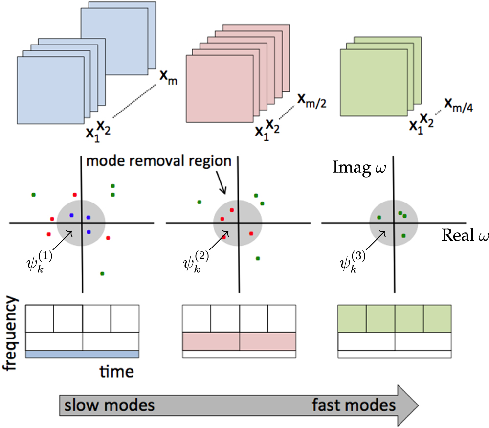
The mrDMD is inspired by the observation that the slow- and fast-modes in the data can be separated [74]. This was originally done in video processing for the application of foreground/background subtraction [99]. The mrDMD algorithm recursively isolates and removes low-frequency content from time-series data. The number of snapshots, M, is typically chosen to capture the relevant range of low-frequency and high-frequency behavior. After an initial pass through the data, the slowest modes are removed, and then the time window is split into two segments with M/2 snapshots each. DMD is performed again on these two smaller snapshot sequences, and the slowest modes are removed from each. The algorithm continues recursively until a desired stopping criterion.
Selecting the slow modes at each level of the mrDMD decomposition is a central consideration. Figure 4 shows the mode selection region as a user chosen threshold to determine which modes are slowly varying on a given decomposition level. Although there are many possible threshold criteria, we define the threshold to select eigenvalues with periods so that a single wavelength or less can fit in the sampling window. As the algorithm continues, the temporal wavelength cutoff is decreased by a factor of two every time the domain is split in half. For a sampling time T, the cutoff frequency is π/T.

Figure 4. Representation of the multi-resolution dynamic mode decomposition where successive sampling of the data, initially with M snapshots and decreasing by a factor of two at each resolution level, is shown (top figures). The DMD spectrum is shown in the middle panel where there are m1 (blue dots) slow-dynamic modes at the slowest level, m2 (red) modes at the next level and m3 (green) modes at the fastest time-scale shown. The shaded region represents the modes that are removed at that level. The bottom panels show the wavelet-like time-frequency decomposition of the data color coded with the snapshots and DMD spectral representations. Reproduced with permission from [74]. © 2016 Society for Industrial and Aplied Mathematics.
Download figure:
Standard image High-resolution image
Figure 5. Schematic of a time-lagged autoencoder type neural network with one nonlinear hidden layer in each the encoding and decoding layers. The encoder transforms a vector  to a d-dimensional latent space while the decoder maps this latent vector et to the vector
  in full coordinate space but at time τ later. For τ = 0, this setup corresponds to a regular autoencoder. Reprinted from [100], with the permission of AIP Publishing.
Download figure:
Standard image High-resolution imageMathematically, the mrDMD separates the DMD approximate solution in the first pass as follows:

where the  represent the DMD modes computed from the full M snapshots.
Figure 4 illustrates the mrDMD process for a three-level decomposition, with the slowest scale in blue, the medium scale in red, and the fastest scale in green. mrDMD is also connected to multi-resolution wavelet analysis, as shown in the bottom panels. The mrDMD solution can be made more precise. Specifically, one must account for the number of levels (L) of the decomposition, the number of time bins (J) for each level, and the number of modes retained at each level (mL). To formally define the series solution for  , we introduce the indicator function

which is only nonzero in the interval, or time bin, associated with the value of j. The parameter ℓ denotes the level of the decomposition.

Figure 6. (a) Example design of a reconfigurable holographic metamaterial antenna with a close-up view of a small section to highlight the arrayed tunable, meta-atoms (b) holographic images on the surface of the array, when illuminated by an underlying feed wave, produce a coherent beam. Different images, encoded by the control pattern applied to each meta-atom, produce beams in different directions. (c) The physics of the metamaterial antenna. The input carrier wave traverses the waveguide, and the meta-atom cells couple energy out of the feed. Further, the cells produce simultaneous amplitude and phase-shift as a function of their control. (d) (top row) Simulated far-field results of the algorithm iteratively targeting different sidelobes while continuously creating a main beam in the direction of 25.7° θ. (bottom row) Representation of the simulated results in a mobile application. © [2015] IEEE. Reprinted, with permission, from [104].
Download figure:
Standard image High-resolution image
The three indices and indicator function (16) give the mrDMD solution expansion

This provides a compact description of the mrDMD decomposition, including information about the decomposition level, time bin location, and the number of modes extracted. The indicator function fℓ, j(t) acts as sifting function for each time bin, as with the Gabór window of a windowed Fourier transform [33]. The hard cut-off in our sampling bin may introduce spurious high-frequency oscillations. However, it is possible to use wavelet functions for the sifting operation, so that the time function fℓ, j(t) can be one of the many potential wavelet basis, i.e. Haar, Daubechies, Mexican Hat, etc.
3.2. Multiscale SINDy
The original SINDy algorithm is well-suited to identify dynamical systems with uniscale dynamics. However, many systems of interest, such as those found in MDs, are fundamentally multiscale, with dynamic coupling at multiple temporal scales. Identifying multiscale dynamics with SINDy would require sampling at a sufficiently small timestep to capture the fastest dynamics while sampling for a sufficient duration to observe the slowest scales. With uniform sampling, this would lead to a tremendous amount of data. Instead, a recent multiscale SINDy algorithm [92] introduces a variable sampling approach to resolve all scales with considerably less data. This approach was demonstrated on a coupled system with two distinct time scales:

In this system  is the set of variables that comprise the fast dynamics, and
  represents the slow dynamics. The linear coupling is determined by our choice of
  , and time constants τfast, τslow, which determine the frequency of the fast and slow dynamics.
With uniform sampling, the data requirement increases approximately linearly with the frequency ratio F = Tslow/Tfast between the coupled systems; Tslow, Tfast are the approximate 'periods' of the slow and fast systems. Thus, the data requirement is considerable for systems where there is a large range of frequencies. By sampling in high-frequency bursts spread out randomly in time, the data requirement stays approximately constant, even with vast timescale separation. By maintaining a small step size in the bursts, we still observe the dynamics in fine detail, and it is possible to estimate the derivative more accurately. By spreading out the bursts, it is possible to sample over a longer duration than would be observed with the same amount of data collected at a uniform sampling rate. Thus, the effective sampling rate is reduced without degrading the derivative estimate or averaging out the fast dynamics. To avoid aliasing, the bursts are spaced randomly, for example triggering the burst sampling with a Poisson process.
4. Applications
In this section, two examples are given where the advocated methods can be applied. The examples are quite different. In the first, the data-driven methods are used to provide a mathematical framework for accelerating MD simulations for materials characterization. In the second, data-driven methods are used for self-tuning of a metamaterial antenna. Both illustrate the possibilities that exist for machine learning integration in materials modeling.
4.1. MD simulations
MD simulations are one of the most common computational tools used for the analysis of the emerging macroscale properties of molecules and materials. The data-driven methods advocated and reviewed here are beginning to migrate into the MD simulation framework, especially for the discovery of low-dimensional models of the long-time dynamics. Frank Noé and co-workers have been recently integrating many of the techniques discussed here in order to produce a principled, innovative suite of algorithms for making tractable long-timescale MD simulations that are interpretable and produce accurate long-time statistics [85, 86, 100–102].
Although there are a variety of aspects of MD that are of research interest, the types of methods presented here are geared towards the discovery and characterization of slow collective variables. These variables are often called reaction coordinates . State-of-the-art methods for identifying slow collective coordinates are based upon the variational approach for conformation (VAC) dynamics. This provides a systematic framework for finding optimal slow collective variables from time-series data. Interestingly, both time-legged embeddings and the DMD have been used to regress to optimal reaction coordinates [100]. Indeed, the time-delay embedding and low-dimensional dynamics can be jointly trained in a time-lagged autoencoder structure in order to exploit many of the features of the dynamics (see figure 5). The autoencoder generalizes the linear embedding of the dynamics to a nonlinear embedding by training a neural network to build a nonlinear feature space on which the dynamics can be projected. The new dynamical representation of the data provides a low-dimensional model which can be used for characterizing MD simulations rapidly and efficiently.
MD simulations are particularly amenable to machine learning innovations as jointly finding low-dimensional subspaces (coordinates) and models which characterize the dynamics of the slow collective variables is of central importance. It also highlights that all the methods presented can leverage the targeted use of neural networks in the data-driven discovery architecture, i.e. finding better coordinates for representing the dynamics. Wehmeyer and Noé demonstrate the use of the time-lagged autoencoder for MD simulations, showing that they can outperform the capabilities of standard linear dimensionality reduction techniques for producing long-time statistical estimates for quantities of interest in the MD. Noé provides an excellent review and comparison of the many machine learning methods available for enhancing MD simulations on long timescales [103]. We encourage the reader to follow this reference for a more comprehensive treatment of state-of-the-art MD simulations embued with machine learning along with simulation codes and data access.
4.2. Metamaterial antennas
Not all materials can be actuated to produce an active and tunable media. However, there is an emerging trend in many application areas to engineer materials that are capable of being modulated by external actuation. For example, metamaterials can be tuned at a microscale in order to produce a desired macroscale response. Such materials allow for adaptable and flexible platforms for applications. They are also ideal candidates for data-driven control strategies and machine learning infrastructures. The DMD and SINDy techniques above may be extended to incorporate control.
The reconfigurable holographic metamaterial surface antenna (MSA) is an emerging technology for satellite communications (see figure 6). The MSA is a low-power device that is flat, thin, and lightweight. Moreover, it achieves active electronic scanning without any mechanical moving parts. However, in order to operate across its entire dynamic-scanning range, the antenna must be able to scan reliably without unacceptable levels of far-field radiation in undesired directions (sidelobes). Thus, it is important to suppress sidelobes while preserving the main beam. In [104, 105], Johnson et al develop an optimization algorithm to suppress sidelobes in the far-field pattern of a MSA in software alone, without the need for nonadaptive hardware modifications.
The MSA is comprised of a planar array of thousands of voltage-tunable meta-atoms that are arranged in a tight rectangular array and fed by a TE10 mode wave propagating in a waveguide beneath the atoms. Because each atom is independently controllable, this provides a tremendous amount of authority to design and steer beams to communicate with satellites. The control space is so high-dimensional that it is not practical to try all combinations of controls in search of good control patterns. Moreover, each atom has a nonlinear phase and amplitude response given a control input. The cells do not display independent amplitude and phase modulation as in a phased array, but instead the amplitude and phase shift occur simultaneously as the control is changed. This resonance behavior is sensitive to manufacturing tolerances. The coupling between the elements and the underlying waveguide further complicates control. All elements are simultaneously slightly changing the feed wave based upon the applied controls. We refer the reader to [104, 105] for more detailed analysis of the types of nonlinear coupling in this antenna system.
It has been shown that extremum-seeking control is well-suited to the dynamic operational requirements of the MSA. In particular, it can optimize the MSA in the field using a pattern synthesis approach to cancel sidelobes while maintaining a strong main beam. Importantly, the control performance is robust to measurement noise and changing environmental conditions. The control is achieved in part by the introduction of an objective function that assesses the performance of the controller. Finally, it is possible to speed-up the optimization using value function approximation [106]. The resulting framework demonstrates that data-driven control can be used as core functionalities for control and analysis of emerging systems where micro scale material properties determine functionality at the macro scale. This work also suggests several future directions, to model, design, and optimize array performance using the data-driven modeling techniques described above.
5. Conclusions and discussion
In this paper, we have reviewed a number of advances in data-driven modeling that we believe will be impactful for (1) MDs, (2) obtaining macroscopic PDEs and constitutive equations for materials, and (3) optimizing and controlling active metamaterials. The modeling techniques described are based on sparse optimization and linear regression, resulting in linear and nonlinear models for systems when full-state measurements or only partial measurements are available. Importantly, techniques for discovering parsimonious models from data greatly improve the prospect of generalizability and interpretability of macroscale models for characterizing material properties. Indeed the combination of deep learning and neural network architectures along with the parsimonious model discovery advocated here provide a rich and compelling theoretical framework for advancing the state-of-the-art in modeling capabilities. Such a diversity of strategies will undoubtedly help advance our understanding and engineering capabilities for developing exotic and improved future materials.
To help researchers start using these emerging methods, we have compiled a list of several recent open-source repositories and other links in table 1. In addition, there is a useful recent review on machine learning in materials [107].
Table 1. Open-source software.
| PyEmma 2: A software package for estimation, validation, and analysis of Markov models (Frank Noe and collaborators [108]) | http://emma-project.org/latest/ |
| Randomized singular value decomposition (rSVD) for large-scale data (N Ben Erichson) | https://github.com/erichson/rSVD |
| SINDy (J-C Loiseau) | https://github.com/loiseaujc/SINDy |
| Sparse regression library for SINDy (Markus Quade) | https://github.com/Ohjeah/sparsereg |
| SINDy and model predictive control (Eurika Kaiser [53]) | https://github.com/eurika-kaiser/SINDY-MPC |
| PDE-FIND (Sam Rudy [58]) | https://github.com/snagcliffs/PDE-FIND |
| Identifying Koopman eigenfunctions (Eurika Kaiser [109]) | https://github.com/eurika-kaiser/KRONIC |
| Deep autoencoder for Koopman eigenfunctions (Bethany Lusch [110]) | https://github.com/mathLab/PyDMD |
| Course on data-driven dynamics (J-C Loiseau) | https://github.com/loiseaujc/Nonlinear_Physics |
| Data-Driven Science and Engineering textbook (video lectures and code on website; Brunton and Kutz [33]) | databookuw.com |
| Dynamic mode decomposition textbook (code on website; Kutz, Brunton, Brunton, Proctor [111]) | dmdbook.com |
Acknowledgments
We are indebted to Kathleen Champion, Mikala Johnson, Eurika Kaiser, and Samuel Rudy for their invaluable contributions in data-driven modeling and control. JNK acknowledges support from the Air Force Office of Scientific Research (AFOSR FA9550-17-1-0329). SLB acknowledges support from the Army Research Office (ARO W911NF-17-1-0306). SLB and JNK acknowledge support from the Defense Advanced Research Projects Agency (DARPA HR0011-18-9-0030).