

Abstract
Understanding the coastal sea level budget (SLB) is essential to revealing the causes of sea level rise and predicting future sea level change. Here we present the coastal SLB based on multiple sets of sea level observations, including satellite altimetry, satellite gravimetry, and Argo floats over 2005 to 2021. The coastal zone is defined within 500 km from the coast and covered by all Argo products. We find that sea level observations enable a closure for the coastal SLB for 2005-2015. However, since 2016, the coastal SLB shows a substantially larger discrepancy, consistent with the global mean SLB. The coastal SLB is unclosed for 2005-2021, with a mean sea level rise of 4.06 ± 0.27 mm yr−1, a 0.74 ± 0.21 mm yr−1 rate for ocean mass, and a 2.27 ± 0.53 mm yr−1 for the steric component. Systematic Argo buoy salinity drift after 2016 is the main cause for the non-closure of coastal SLB over 2005-2021. Ignoring the suddenly unrealistic coastal salinity trends, the global coastal SLB from 2005 to 2021 is closed with a residual trend of 0.46 ± 0.63 mm yr−1. Our results confirm that the coastal 500 km range does not need to be deliberately masked and ignored in global SLB research.
Export citation and abstract BibTeX RIS

Original content from this work may be used under the terms of the Creative Commons Attribution 4.0 licence. Any further distribution of this work must maintain attribution to the author(s) and the title of the work, journal citation and DOI.
1. Introduction
Monitoring the coastal sea level changes is of great importance since nearly half of the world's inhabitants reside within 100 km of the coast (Vignudelli et al 2019). The sea level rise continues to threaten human infrastructure in coastal areas, not only threatening the survival of coastal residents, but also destroying fragile coastal ecosystems (IPCC 2021). Moreover, extreme weather events like storm surges are becoming more frequent and intensified, which exacerbate the vulnerability of coastal regions (Dodet et al 2019, Muis et al 2020). It is virtually certain that a greater proportion of human beings will be exposed to the hazards of coastal sea level rise in the near future. Therefore, it is of great significance to understand the causes of sea level rise in coastal regions (Fenoglio-Marc and Tel 2010, Nicholls et al 2010, Mu et al 2019, Qu et al 2019, Vignudelli et al 2019, Woodworth et al 2019, Xu et al 2019, Benveniste et al 2020).
In recent years, satellite altimetry technology represented by TOPEX, Jason altimeters, satellite gravimetry technology represented by Gravity Recovery and Climate Experiment (GRACE) and GRACE-FO, and ocean temperature and salinity sampling technology represented by Argo buoys have greatly improved our understanding of the causes of sea level change. These three types of observation techniques constantly monitor global sea level change as well as the steric component, caused by the ocean temperature and salinity change, and the mass component, caused by the mass exchange between oceans and land. Numerous studies have quantified the contribution of each component to sea level rise over different time spans, and many of them have closed the sea level budget (SLB) for the trend term (WCRP 2018, Frederikse et al 2020, Royston et al 2020, Wang et al 2021, Camargo et al 2022, Yang et al 2022).
However, most experts mask and ignore the coastal regions, an area hundreds of kilometers from the coastline, when investigating global mean sea level change or global mean ocean mass changes. One reason is probably because these three types of data have insufficient coverage in the coastal regions. The coastal SLB is therefore a major challenge in the field of climate change. Technically, the difficulties of determining the causes of coastal sea level budget include following aspects. First, during the GRACE data processing, spatial filtering will lead to significant leakage errors at the sea-land boundary, and the leakage signal from land into the ocean may obscure the real ocean mass changes. Second, affected by land-reflected signals , sea-state bias and ocean tide corrections, the data quality of satellite altimetry is poor over the coastal areas (Laignel et al 2023). Finally, Argo buoys are insufficiently sampled in coastal regions, such as the South China Sea, the Sura Sea, the Mexican Basin, and the Caribbean Sea.
To address these issues, experts have been exploring ways to improve resolution for coastal areas by proposing new data processing methods. The altimetry community improved data processing algorithms, background field models, and software for coastal areas to increase the spatial coverage of altimetric data within the 5 km coastline (Birol et al 2017, Birol et al 2021). Joen et al (2021) investigated the SLB in several typical coastal regions from 2005-2015, and found that the GRACE spherical harmonic solution (SHs)with the forward modeling (FM) method outperforms the Mascon solution in these regions, while Mascon products differed more in small-scale coastal areas (Jeon et al 2021). Chang et al (2021) studied the causes of sea level change in the China Sea, and compared the relationship between sea level change and ENSO. Xu et al (2022) found that GRACE and Argo observations can well explain satellite altimetry observations on both seasonal and non-seasonal scales within 300 km coastal regions from 2002 to 2020, but the coastal SLB is not closed, with a ∼1 mm yr−1 difference in the trend budget.
However, we note that most experts focus on relatively small-scale research on the causes of coastal sea level changes. The coastal SLB within the 500 km range from the coastline requires further study, especially for the part of the area already included in the global gridded product. In addition, whether the drift of Argo salinity data, officially reported to be caused by the failure of some seabird buoys after 2016, affects coastal sea level change needs further confirmation. This study uses multiple sets of satellite altimetry, satellite gravimetry and ocean temperature and salinity data to study the trend budget of global coastal sea level. The paper is structured as follows: section 2 provides a brief introduction to the data and methodology; section 3 presents the global coastal mean SLB. Section 4 discusses the reasons for the non-closure of coastal SLB after 2016. Section 5 is the conclusion of this paper.
2. Data and methodology
This section briefly introduces the three types of observational data used in this study, including 3 sets of altimetry sea level anomaly products, 12 sets of Argo temperature and salinity fields, and 6 sets of GRACE/GRACE-FO data products, which are used to calculate total sea level change, steric sea level change and ocean mass change, respectively. Table 1 lists information on the datasets used in this study, including spatial and temporal resolution, time span, and reference.
Table 1. Summary of data sets used to calculate coastal sea level change. "d/o" is the abbreviation for SHs degree/order.
| Category | Institute | Resolution | Time period | Reference |
|---|---|---|---|---|
| Altimetry | CMEMS | 1/4°× 1/4° grid, monthly | 1993.01-2022.05 | https://marine.copernicus.eu/ |
| JPL | 1/6°× 1/6° grid, 5-day | 1992.10-2022.12 | (Fournier et al 2022) | |
| CSIRO | 1° × 1° grid, monthly | 1993.01-2020.07 | http://cmar.csiro.au/ | |
| ARGO | BOA | 1° × 1° grid, 58 levels to 1975 dbar, monthly | 2004.01-2022.09 | (Li et al 2017) |
| CORA | 1/2°× 1/2° grid, 152 levels to 2000 m, monthly | 1990.01-2021.12 | (Cabanes et al 2013) | |
| EN4 | 1° × 1° grid,42 levels to 5350 m, monthly | 1900.01-2023.01 | (Levitus et al 2009, Cowley et al 2013, Good et al 2013, Cheng et al 2014, Gouretski and Cheng 2020) | |
| IAP | 1° × 1° grid,41 levels to 2000 m, monthly | 1940.01-2022.12 | (Cheng et al 2017) | |
| IPRC | 1° × 1° grid,27 levels to 2000 m, monthly | 2005.01-2020.12 | http://apdrc.soest.hawaii.edu/ | |
| ISAS | 1/2°× 1/2° grid,187 levels to 5500 m, monthly | 2002.01-2020.12 | (Gaillard et al 2016, Kolodziejczyk et al 2021) | |
| JAMSTEC | 1° × 1° grid, 25 levels to 2000 dbar, monthly | 2001.01-2022.06 | (Hosoda et al 2010) | |
| NCEI | 1° × 1° grid, 137 levels to 5500 m, 3-month | 2005.01-2022.12 | (Levitus et al 2012) | |
| SIO | 1° × 1° grid, 58 levels to 1975 dbar, monthly | 2004.01-2022.12 | (Roemmich and Gilson 2009) | |
| GRACE | CSR | 60 d/o SHs, monthly | 2002.04-2022.11 | https://2.csr.utexas.edu/ |
| (Pie et al 2021) | ||||
| GFZ | 60 d/o SHs, monthly | 2002.04-2022.11 | https://gfz-potsdam.de/ | |
| JPL | 60 d/o SHs, monthly | 2002.04-2022.11 | https://podaac.jpl.nasa.gov/ | |
| ITSG | 60 d/o SHs, monthly | 2002.04-2022.12 | (Kvas et al 2019) | |
| JPL-M | 1/4°× 1/4° grid, monthly | 2002.04-2022.11 | (Watkins et al 2015) | |
| CSR-M | 1/4°× 1/4° grid, monthly | 2002.04-2022.10 | (Save et al 2016) |
The measurements of total sea level change are taken from satellite altimetry. Since 1993, a series of satellites equipped with altimeters have been launched to monitor global sea level changes. This study mainly uses the global grid sea surface height anomaly products released by three institutions: the Copernicus Marine Environment Monitoring Service (CMESM), the Jet Propulsion Laboratory (JPL, version 2205), and the Commonwealth Scientific and Industrial Research Organisation (CSIRO). These products combine all available altimetry missions with a series of corrections. Before joint calculations with satellite gravimetry and ocean temperature and salinity data, glacial isostatic adjustment (GIA) has been applied based on the model ICE6G-D, while ocean bottom deformation (OBD) corrections are calculated based on GRACE SHs and loading theory (Peltier et al 2018, Vishwakarma et al 2020).
The steric contribution is mainly estimated from Argo products. Since 2001, the Argo program has become a major component of the global ocean observation system, providing ocean observation elements such as temperature, salt (depth above 2 000 m). This study mainly used 12 gridded ocean temperature and salinity datasets released by the following institutions: Second Institute of Oceanography (BOA), the Coriolis Ocean database for ReAnalysis (CORA), the Met Office Hadley Centre for Climate Change (EN4 series products, version 4.2.2, named EN4_g10, EN4_l09, EN4_c13, EN4_c14), the Institute of Atmospheric Physics in China (IAP), the International Pacific Research Center (IPRC), the Laboratory for Ocean Physics and Satellite remote sensing (ISAS, version ISAS20_ARGO), the Japan Agency for Marine-Earth Science and Technology (JAMSTEC), the National Centers for Environmental Information (NCEI), and the Scripps Institution of Oceanography (SIO). The primary data source for these datasets is Argo buoy observations, some of these datasets also comprehensively consider other ocean observations such as CTD and XBT. Besides, Thermodynamic equation of Seawater (TEOS‐10) is used to calculate the steric change (McDougall and Barker 2011), and we only integrate to 2000 m depth for all gridded products.
Ocean mass variations are determined from GRACE and GRACE-FO. Since March 2002, the GRACE/GRACE-FO gravity satellite has provided global time-varying gravity field data. This study uses Level-2 RL06.1 SHs provided by the Center for Space Research (CSR), the German Research Centre for Geosciences (GFZ), JPL,and the Institute of Geodesy at Graz University of Technology (ITSG) and Level-3 Mascon products provided by JPL and CSR (named JPL-M and CSR-M). In order to obtain ocean mass change, spherical harmonic coefficient products need to undergo low-order term replacement, GIA correction, Gaussian filtering, leakage error correction, seismic effect elimination, IB correction, etc (Wahr et al 1998, Swenson et al 2008, Johnson and Chambers 2013, Sun et al 2016, Cheng and Ries 2017, Peltier et al 2018, Uebbing et al 2019), while mascon products do not require complex inversion calculations. Note that as a complement to the global SLB in the cosatal region, we still use the classical approach proposed by Wahr et al (1998) to correct the leakage error, without resorting to other land water models.
This study uses the average trend of multiple sets of products as the final trend estimate and the combined error as the uncertainty estimate (Uebbing et al 2019, Royston et al 2020, Yang et al 2021). The combined error generally includes the trend uncertainty of the linear fitting calculation, the ensemble spread caused by the selection of the different data sets, and the spread errors generated by the selection of different correction products during data processing. The uncertainties of the altimetry orbit and OBD used here are referring the work of Royston et al (2020). More detailed information of the uncertainty quantification can be found in section 2 in Yang et al (2022). The necessary linear interpolation was adopted to reconcile the spatial resolution of the dataset to 1°× 1, while the monthly averaging was used to match the JPL altimetry dataset with the other datasets. The definition of the coastal ocean in this study is shown in figure 1, extends up to 500 km away from the coastline and covered by the three types of data. Considering the possible leakage errors and significant GIA effects caused by GRACE/GRACE-FO data processing in polar regions, polar sea areas where ocean mass cannot be accurately quantified are not included in the scope of this study. Considering the common period for most of the datasets and the global coverage of Argo buoys until 2005, we focus on the coastal sea level change from 2005 to 2021. Note that the datasets CSIRO, IPRC, and ISAS are not updated to 2021, so these datasets were only used to calculate the ensemble average and the trend for 2005-2015. We assume that the halosteric trend difference between the period of 2005–2021 and 2005–2015 is the impact of salinity drift after 2016.
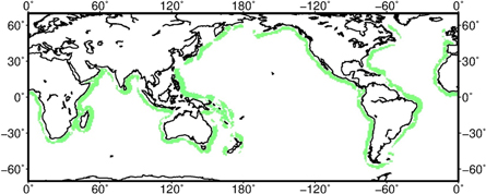
Figure 1. The coastal ocean defined in this study (500 km from the coastline, excluding polar regions).
Download figure:
Standard image High-resolution image3. Results
Figure 2 shows the time series of coastal mean sea level and its components. From 2005 to 2021, the global coastal mean sea level has risen significantly, which is caused by both increase of ocean mass and steric components. Among them, the ocean mass component shows a strong linear increase, while the inter-annual change of the steric component is more obvious. Since 2005, the cumulative global coastal mean sea level has risen by ∼80 mm, of which the ocean mass component has contributed ∼30 mm, and the steric component has contributed ∼30 mm. The sea level series reconstructed by GRACE and Argo are in good agreement with the altimetry observations, especially during the period 2005 to 2015 when the quality of the observations was particularly good. The correlation coefficient between the mean reconstructed series from multiple sets of data and the measured series exceeds 0.95. It can be seen from the residual series of SLB that the ∼20 mm sea level rise after 2016 cannot be reasonably explained. From 2005 to 2016, the coastal SLB residual fluctuated around zero, while the residual showed a 'significant' increase trend after 2016. This phenomenon is consistent with sea level changes at the global and basin scales, which is mainly due to the systematic drift of salinity experienced by Argo since 2016 and the uncertainty of the wet tropospheric delay bias of the Jason-3 altimetry satellite (Chen et al 2020, Barnoud et al 2021, Yang et al 2022).

Figure 2. Time series of the coastal mean sea level (SSH, black curve), the steric sea level change of the upper 2000 m (Steric, blue curve), the ocean mass change (Mass, green curve), the sea level budget residual (Residual, red curve), and sea level change reconstructed from mass and steric components (Reconstructed, cyan curve). The solid line represents the multi-dataset average and the corresponding shaded area is the standard deviation. Seasonal signals are removed and 3-month smoothing applied.
Download figure:
Standard image High-resolution imageTable 2 summarizes the global coastal sea level change rates for 2005-2015 and 2005-2021, including multi-dataset average and corresponding uncertainties. From 2005 to 2015, the global coastal sea level rise rate was about 4.63 ± 0.48 mm yr−1, which exceeded the global average (3.24 ± 0.53 mm yr−1) for the same period. The contribution of ocean mass component is 2.58 ± 0.53 mm yr−1, while the steric component is 1.70 ± 0.41 mm yr−1, and the residual trend of the coastal SLB is 0.35 ± 0.82 mm yr−1 for the 2005-2015 period. From 2005 to 2021, the global coastal sea level rise rate was about 4.06 ± 0.27 mm yr−1, slightly slower than the rise rate from 2005 to 2015. The contribution of the ocean mass component is about 2.27 ± 0.53 mm yr−1, while the steric component is significantly slowed down by 0.74 ± 0.21 mm yr−1, and the residual trend of the SLB is 1.05 ± 0.63 mm yr−1 for the 2005-2021 period. The coastal sea level change was well explained by the mass and steric components from 2005 to 2015, and the residual trend of the SLB was much smaller than its uncertainty. From 2005 to 2021, the global coastal SLB was not closed significantly, and the sea level change reconstructed by GRACE and Argo is much lower than sea level change derived from altimetry.
Table 2. Coastal sea level change and trends and uncertainty statistics (mm/yr).
| 2005–2015 | 2005–2021 | ||||
|---|---|---|---|---|---|
| Altimetry | |||||
| Mean Trend | ±s.e. | 4.63 | 0.24 | 4.06 | 0.14 |
| ensemble spread | 0.36 | 0.10 | |||
| orbital altitude | 0.13 | 0.13 | |||
| OBD | 0.16 | 0.16 | |||
| GIA spread | 0.05 | 0.05 | |||
| Quadratic sum of uncertainties | 0.48 | 0.27 | |||
| Argo | |||||
| Mean Trend | ±s.e. | 1.70 | 0.25 | 0.74 | 0.15 |
| ensemble spread | 0.32 | 0.14 | |||
| Quadratic sum of uncertainties | 0.41 | 0.21 | |||
| GRACE | |||||
| Mean Trend | ±s.e. | 2.58 | 0.10 | 2.27 | 0.07 |
| ensemble spread | 0.41 | 0.37 | |||
| degree1 spread | 0.01 | 0.01 | |||
| C20 spread | 0.06 | 0.09 | |||
| GIA spread | 0.29 | 0.29 | |||
| filter spread | 0.13 | 0.22 | |||
| Quadratic sum of uncertainties | 0.53 | 0.53 | |||
| Altimetry-GRACE-Argo | 0.35 | 0.82 | 1.05 | 0.63 | |
| Coastal salinity drift | 0.59 | ||||
| Revised residual trend | 0.46 | 0.63 | |||
Figure 3 summarizes the coastal sea level trends for each dataset of altimetry, Argo and GRACE/GRACE-FO. Various combinations of data products and post-processing strategies will lead to different trend values and SLB results. From 2005-2015, the rate of coastal sea level rise of JPL exceeded CMEMS and CSIRO by 0.5 mm yr−1, while the latter two agencies have very similar trend values. However, the differences between these datasets are almost negligible during the Jason-3 satellite period, and the subjective selection of altimetry data products has little effect on trend value for 2005-2021. The coastal SSH trends are not highly sensitive to orbital altitude and OBD products. The choice of the Argo data center has a very significant impact on the coastal steric sea level trends. According to the temperature-salinity field data released by different institutions, coastal steric sea level trends discrepancies can be up to ±0.8 mm yr−1, ±0.25 mm yr−1 for 2005-2015 and 2005-2021. In addition, it is impossible to judge which set of Argo products is more reliable (Dieng et al 2015, Camargo et al 2020), we recommend using multiple sets of data averaging.
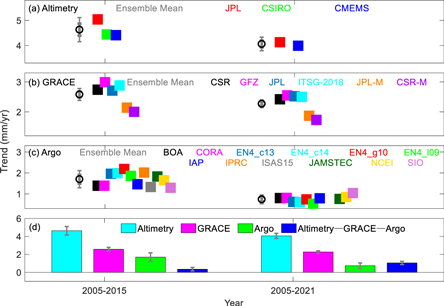
Figure 3. Statistics of coastal mean sea level change trends, including individual datasets and integrated averages. (a) Altimetry, (b) GRACE, (c) Argo, (d) SLB. The error bars represent the error of the least squares linear fit (95% confidence level). Note that the datasets CSIRO, ISAS and IPRC are not updated to 2021.
Download figure:
Standard image High-resolution imageThe ocean mass change calculated by the GRACE/GRACE-FO Mascon solution is much smaller than that of the spherical harmonic solution because the leakage error correction strategies are different for these products. The uncertainty range of these two solutions can reach up to ±0.88 mm yr−1. The spread in ocean mass trends between different post-processing corrections is relatively smaller. From the perspective of the closure of the SLB, the spherical harmonic solution can make the coastal SLB closer to closure, which means that the mascon solution may underestimate the ocean mass changes in coastal area. Another similar conclusion appears in Jeon et al (2021), who found the spherical harmonic solution corrected for leakage error explains the coastal SLB better than mascon solutions over six selected coastal regions. Although the FM leakage error correction method they used may be more applicable to small-scale coastal regions, the conventional leakage error correction method often used for global-scale studies is sufficient to close the global coastal SLB.
In addition to the causes of trend changes, detrended terms are also important factors in understanding coastal sea level changes. The mean correlation between the non-trend series of the reconstructed coastal sea level and the corresponding non-trend altimetry series is only 0.69, which means that the mass and steric changes cannot well explain the variability in the altimetry records. This finding seems to contradict the results of Xu et al (2022) who found that the reconstructed (EN4 + CSR) and observed (CMEMS) sea surface heights differed significantly in the trend terms, while the non-trend change matched better. But it reflects the variability between data sets. In other words, the subjective selection of the datasets can seriously affect analysis of the causes of sea level change. For example, the correlation between CMEMS and EN4 + CSR combination is as high as 0.9 (Xu et al 2022), while the correlation coefficients for most combinations here are less than 0.7.
4. Discussion
Since 2016, the rate of steric sea level change has decreased by about 1 mm yr−1 (table 2). Is the significant decline (which mainly reflects a decline in upper steric sea level change) caused by the real signal or by the Argo salinity data drift? figure 4 presents the global coastal mean steric sea level anomalies (SSLA), thermosteric sea level anomalies (TSLA), and halosteric sea level anomalies (HSLA). Since temperature dominates the total steric change, the coastal mean time series of SSLA and TSLA show a consistent oscillating upward trend. However, there is a large interannual variation difference between various datasets, and even individual datasets have obvious 'errors', such as the IPRC dataset, where the steric change deviates significantly from the mean for multiple months, especially after 2018. Therefore, the IPRC dataset is not suitable for calculating the ensemble average trend for 2005-2021. After 2019, except for significant drop of SSLA and TSLA in IPRC, the other datasets show a consistent upward trend.
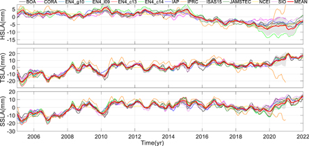
Figure 4. Time series of global coastal mean steric sea level anomalies (SSLA), thermosteric sea level anomalies (TSLA), and halosteric sea level anomalies (HSLA). Note that the HSLA series of the EN4 products are overlapping.
Download figure:
Standard image High-resolution imageNote that the differences in the EN4 series datasets are mainly due to the different methods of bias correction for the temperature profile data. Thus, their HSLA series are completely overlapping, while the TSLA and SSLA series are distinctly different. Compared to the other datasets, each EN4 dataset has a smaller HSLA trend, a larger TSLA trend, and a slightly smaller SSLA trend after summation. Removing a single or full series of EN4 datasets does not inherently affect the results of ensemble mean trends.
From 2005 to 2015, the HSLA series remained fluctuating around '0', and the amplitude did not exceed 5 mm. After 2016, the majority of HSLA showed a clear downward trend, with an average decrease of ∼10 mm. The HSLA sequence of individual data even cumulatively dropped by more than 20 mm in 2020, while the HSLA of IPRC increased by 5 mm during this period. It is apparent that the salinity data published by various institutions varies widely. So, the HSLA trends and SLB are most affected by the choice of Argo product especially after 2016.
As depicted in figure 5, global coastal mean TSLA increases by 1.33 to 2.31 mm yr−1 for different data from 2005 to 2015. Since the HSLA trend is not significant, the TSLA trend value can generally replace the SSLA. However, the increasing trend of TSLA and SSLA slowed down from 2005 to 2021. In addition, HSLA shows a consistently significant negative trend, both for individual datasets and ensemble averages. The average HSLA rate was −0.59 ± 0.14 mm yr−1, which has reached an order of magnitude that cannot be ignored. The slowing down of the warming effect of the upper ocean, coupled with the offsetting effect of ocean saltiness, led to a significant decrease in SSLA after 2016.

Figure 5. Global costal mean trends for steric sea level anomalies (SSLA), thermosteric sea level anomalies (TSLA), and halosteric sea level anomalies (HSLA). The error bars represent the error of the least squares linear fit (95% confidence level). Note that the datasets ISAS and IPRC are not updated to 2021.
Download figure:
Standard image High-resolution image
According to the HSLA trends from 2005 to 2015, the global coastal salinity changes are negligible. The Argo salinity data drift has seriously affected the global coastal mean SLB from 2005 to 2021, with a magnitude of up to 0.59 mm yr−1. Therefore, when making the coastal SLB, the salinity change should not be considered, and TSLA can be directly used instead of SSLA for calculation. From 2005 to 2021, the corrected residual of the global coastal SLB was 0.46 ± 0.63 mm yr−1, which also means that the coastal SLB is closed. This explains the coastal SLB trend discrepancy of ∼1 mm yr−1 found by Xu et al (2022): (1) the influence of salinity drift is not considered; (2) the data source used is relatively single; and (3) the assessment of errors may not be comprehensive enough.
According to the report from Argo Program Office, more and more Argo floats have drifted salinity since 2015 (https://argo.ucsd.edu/). The Seabird CTD cell (serial number 6000-7100 and 8100-9200) equipped on the Argo buoy has experienced high salinity drift, exceeding the nominal 0.01 PSU-78 accuracy (Wong et al 2020, Barnoud et al 2021). Our study also illustrates that these equipment failures have affected global coastal regions. Effective measures are being implemented to reduce the effects of drift, such as recalling some of the problem buoys, improving manufacturing, and flagging the erroneous salinity profiles. As shown in figure 4, the drift of HSLA is slowly decreasing. In addition, the SIO dataset (Roemmich and Gilson 2009) was produced using WOCE Global Hydrographic Climatology data for the salinity drift revision, and therefore its salinity drift is minimal after 2016.
The coastal SLB is more difficult to be revealed, compared to the global average. The selection of data sets and processing strategies may significantly affect the sea level estimation. Therefore, we recommend to use as many sets of data as possible when doing such research. Due to the limited resolution by data sampling, the spatial distribution of the coastal trend is not shown. Our results suggest that our coastal region can be included when conducting global SLB studies. Of course, the polar regions beyond our definition of coastal ocean still require further investigations.
5. Conclusions
This study uses 3 datasets of satellite altimetry, 6 datasets of satellite gravimetry and 12 datasets of ocean temperature and salinity data to investigate the causes of coastal sea level change from 2005 to 2021. The coastal mean sea level has been rising significantly, with a rate of about 4.06 ± 0.27 mm yr−1, of which the contribution of ocean mass and steric component is 2.27 ± 0.53 mm yr−1 and 0.74 ± 0.21 mm yr−1 respectively. The residual trend of coastal SLB is 1.05 ± 0.63 mm yr−1.
From 2005 to 2021, the coastal SLB was not closed, mainly due to the systematic drift of Argo buoy salinity data after 2016. According to the 2005-2015 HSLA trends, the global coastal salinity changes are theoretically negligible to SLB. When ignoring changes in salinity, the global coastal SLB from 2005 to 2021 is closed with a residual trend of 0.46 ± 0.63 mm yr−1. Therefore, it is not necessary to mask the coastal 500 km range in future research on the global SLB.
Acknowledgments
The authors are very grateful for constructive comments and guidance from three anonymous reviewers. We would like to thank the institutions or authors listed in table 1 for their data support. This work was supported by the National Natural Science Foundation of China (41904081, 42004073, 42027802, and 42192534), the State Key Laboratory of Geodesy and Earth's Dynamics, Chinese Academy of Sciences (SKLGED2022-2-1).
Data availability statement
All data that support the findings of this study are included within the article (and any supplementary files).