

Abstract
Heat wave events usually cause disastrous consequences on human life, economy, environment, and ecosystem. However, current climate models usually perform poorly in forecasting heat wave events. In the current work, we identified that the leading mode of the summer (June-July-August) heat wave frequency (HWF) over the Eurasian continent (HWF_EC) is a continental-scale pattern. Two machine learning (ML) models are constructed and used to perform seasonal forecast experiments for the summer HWF_EC. The potential predictive sources for the HWF_EC are chosen from the fields related to the lower boundary conditions of the atmosphere, i.e., the sea surface temperature, snow cover, soil moisture and sea ice. The specific regions and months of these lower boundary condition fields selected to construct the potential predictors are those that are persistently and significantly correlated with the variation in the HWF_EC preceding the summer. The ML forecasting models are trained with data from the period 1980–2009 and then used to perform real seasonal forecasts for the summer HWF_EC for 2010–2019. The results show that the ML forecasting models have reasonably good skills in predicting the HWF_EC over high HWF regions. The two ML models show obviously better skill in the forecasting experiments than a traditional linear regression model, suggesting that the ML models may provide an additional and useful tool for forecasting the summer HWF_EC.
Export citation and abstract BibTeX RIS

Original content from this work may be used under the terms of the Creative Commons Attribution 4.0 licence. Any further distribution of this work must maintain attribution to the author(s) and the title of the work, journal citation and DOI.
1. Introduction
Heat wave events are usually associated with persistent anomalous high-pressure systems, which can cause abnormally warm conditions through excessive adiabatic warming resulting from increased downward motion and the increasing absorption of solar radiation caused by decreased cloud cover (Pezza et al 2012, Marshall et al 2014, Boschat et al 2015). The anomalous high-pressure systems associated with heat wave events vary among different regions. Over tropical and subtropical regions, subtropical highs are responsible for many heat wave events (Parker et al 2014a, Parker et al 2014b). The midlatitude blocking highs associated with quasi-stationary Rossby waves have played a primary role in numerous heat wave events over the Eurasian continent, including those in 2003, 2010 and 2018 (Meehl and Tebaldi, 2004, Otto et al 2012, Vautard et al 2013, Kueh and Lin, 2020). Previous work has demonstrated that many other boundary conditions, including sea surface temperature (SST) (Sutton and Hodson, 2005, Feudale and Shukla, 2011), soil moisture (SM) (Fischer et al 2007, Vautard et al 2007), snow cover (SC) (Wu et al 2012, 2016), sea ice (SI) (Wu et al 2013, Wu and Francis, 2019) and greenhouse gases (Angélil et al 2014, Sun et al 2014), may contribute to extreme temperature events through different physical processes.
Under the background of global warming, many regions throughout the Eurasian continent have experienced heat wave events with stronger intensities and longer durations more frequently during the last several decades (Schär et al 2004, Matsueda, 2011, Zhang and Wu, 2011, Sun, 2014, Perkins, 2015, Yang et al 2021). Some climate model projections reported high possibilities of increases in the duration, intensity and frequency of heat wave events under enhanced greenhouse gas conditions (Stocker, 2014, Tangang et al 2018, Li, 2020, Kotharkar and Ghosh, 2021), while others have noted that such increases are spatially heterogeneous (Fischer and Schär, 2008, Fischer and Schär, 2010, Sun et al 2014). As heat wave events can have disastrous consequences for many components of everyday life, including human health, society, tourism, the environment, and ecosystems, understanding the dynamics and improving the forecast skill of heat wave events are therefore of great importance to government and industry contingency planners (Dunstone et al 2019, Wulff and Domeisen, 2019).
Recently, some real-time forecasts of extreme temperature events have been performed using climate models at different time scales ranging from subseasonal to seasonal and even interdecadal variations (Sun et al 2014, Tangang et al 2018, Shafiei Shiva and Chandler, 2020). In general, climate models perform poorly in forecasting extreme temperature events (Quandt et al 2017, Vitart and Robertson, 2018, Kueh and Lin, 2020). Nevertheless, while forecasting heat wave events a couple of months in advance is difficult, some characteristics, such as the heat wave frequency (HWF) or heat wave intensity, might be predictable. Accordingly, reasonable predictions of the characteristics of these extreme temperature events may provide useful information for the government and policy makers.
With the development of computer science, machine learning (ML) models have played an increasingly important role in climate forecasting (Badr et al 2014, Chi and Kim, 2017, Cohen et al 2019, Hwang et al 2019). Some previous works have demonstrated that ML models perform comparably well or even better in seasonal forecasting than complex dynamic climate models over some regions (Ham et al 2019, Qian et al 2020). However, how well ML models can forecast some characteristics of extreme climate events on a seasonal time scale remains unclear. The present work examines the forecast skill of a continental-scale summer (June-July August) HWF over the Eurasian continent (HWF_EC) using two ML models, i.e., the light gradient boosting machine (LightGBM) and categorical feature support in gradient boosting (CatBoost), for the HWF_EC during the period 1980–2019.
2. Data and models
The following datasets are used in this work:
- (1)Daily maximum temperature anomalies are obtained from the Global Historical Climatology Network-Daily (GHCND) gridded dataset (HadGHCND) produced through a joint effort between the United States National Oceanic and Atmospheric Administration (National Climatic Data Center) and the United Kingdom's Hadley Centre. Its temporal coverage ranges from 1950 to the present with a regular spatial resolution of 2.75 × 2.5 (Caesar et al 2006).
- (2)SC data are acquired from the Rutgers University Global Snow Laboratory Northern Hemisphere Weekly Snow Cover Extent Dataset (Robinson and Estilow, 2012), which has a horizontal resolution of 25 km and covers the period from October 1966 to the present. To facilitate the analysis, the data are converted into monthly mean data following (Wang et al 2018).
- (3)Monthly mean sea surface temperature and sea ice concentration data gridded at a resolution of 1 × 1 and covering the period from 1870 to the present are obtained from the Met Office Hadley Center (Rayner et al 2003).
- (4)Monthly mean 200 hPa geopotential height (Z200) and SM (10–200 cm) data from January 1979 to the present are obtained from the National Centers for Environmental Prediction (NCEP)-Department of Energy (DOE) Reanalysis II (Kanamitsu et al 2002).
The LightGBM model (Ke et al
2017) and the CatBoost model (Prokhorenkova et al
2018) are used to perform seasonal forecasting in the present work. These two ML models are different algorithm implementations based on the gradient boosting decision tree (GBDT), which is a very popular and effective algorithm model (Liang et al
2020). With their effective training rate and high precision rate, both ML models have shown reasonable forecasting performances in previous work (Fan et al
2018, Song et al
2019, Liang et al
2020, Shahriar et al
2021). In addition, both algorithms are tree ensemble ML models, which means that the contribution of each predictor to the forecast can be evaluated. The contribution of each predictor is evaluated following Brieman et al (1984). More detailed introduction to the tree ensemble ML models and the contribution assessment method can be found in
3. Methods
In this study, heat wave events are defined using the daily maximum temperature data of summer (June-June-August) for the period 1980–2019. Following Fischer and Schär (Fischer and Schär, 2010), a heat wave event is chosen when the daily maximum temperature exceeds the respective calendar-day 90th percentile and persists for at least six consecutive days. Considering the seasonal cycle, at each grid point, the 90th percentile is calculated with a centered 15-day-long time window for each calendar day. With a moving window, the temporal dependence of each heat wave event is accounted for, and the sample size is reasonable to calculate a realistic percentile value (Wu et al 2016). In the present work, the HWF of a grid point over the Eurasian continent (15°W-175°E, 5°S-80°N), namely, the HWF_EC, for summer is calculated as the sum of the total number of days of the selected heat wave events from June through August.
The method used to perform the seasonal forecast follows (Qian et al 2020, 2021). According to an empirical orthogonal function (EOF) analysis, the HWF_EC can be decomposed into EOF (spatial patterns) modes and their corresponding principal components (PCs, time series) as follows:

where  denotes the spatial structure of the
  -th EOF of the summer HWF_EC and
  is the corresponding time series.
  represents the number of EOF modes. In the present work, the leading EOF (EOF1) of HWF_EC is used, and its corresponding time series is PC1, which is predicted using both ML models. In the forecast, the HWF_EC is constructed according to equation (1) using EOF1 obtained from the observations and PC1 predicted by the ML models.
Note that we conduct the EOF analysis of the summer HWF_EC for the period 1980–2019 to investigate the variation and the continental-scale pattern of HWF_EC in section 4. Hereafter, considering the artificial prediction skills that may be caused by the predictors based on high correlation with the predictand (DelSole and Shukla 2009, Zhao et al 2021), the EOF1 and PC1 obtained using 30 years (1980–2009) of summer HWF_EC data are used in the following analysis, which are quite similar to the 40-year results. Then, PC1 is employed to select the potential predictors to construct the ML models. The retained data for the period 2010–2019 are used to conduct the real-time forecast, i.e., retrospective cross-validation of the forecast models. Detailed results will be presented in section 5.
An exhaustive grid search with a cross validation algorithm (Huang et al 2012) is conducted to choose the hyper-parameters of the two ML models used in our work. This method exhaustively generates candidates, i.e., the parameter combinations, from a grid of parameter values. We choose some important hyper-parameters to conduct grid search, and the others are set to default (i.e., the number of boosted trees, maximum tree leaves for base learners, boosting learning rate and the subsample ratio of the training instance). Considering the limited number of samples that can be used to train the ML models, a fivefold cross-validation method is used to evaluate the ML models. Specifically, the training data of 1980–2009 are split into five smaller sets. Then, four of the folds are used as training data for the ML models, and the remaining fold of data is used to validate the ML models. The metric used to evaluate the performance of the models is the averaged root mean square error (RMSE) computed in the loop. In the real-time forecast experiment, the evaluation of the selected hyper-parameters and trained ML model is measured using the datasets of 2010–2019.
4. Summer HWF over the eurasian continent
Figure 1(a) shows the spatial distributions of the climatology (shading) and the standard deviation (contour) of the summer HWF_EC for the period 1980–2019. Three high-HWF regions can be observed over Europe (0°−82°E, 32°−68°N, EUR), Southeast Asia (93°−128°E, 8°−34°N, SEA) and Northeast Asia (120°−170°E, 50°−75°N, NEA) (denoted by the three blue rectangular boxes in figure 1(a)). Accordingly, three HWF indices are constructed for EUR (HWFI_EUR) (figure 1(c), red line), SEA (HWFI_SEA) (figure 1(c), blue line) and NEA (HWFI_NEA) (figure 1(c), green line) by taking the weighted-area average of the HWF in the three rectangular boxes. The three HWF indices are significantly correlated with each other, with temporal correlation coefficients (TCCs) ranging from 0.31 to 0.55, all significant at the 95% confidence level, suggesting that the summer HWF over the Eurasian continent is a continental-scale pattern and may be impacted by some continental-scale atmospheric circulations.
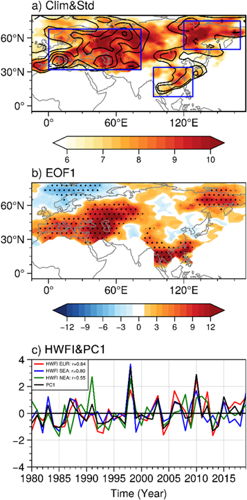
Figure 1. (a) The spatial distributions of the climatology (shading, unit: day) and standard deviation (contour, unit: day) of the HWF_EC for the period 1980–2019. The three blue rectangular boxes denote the three key regions of the HWF over EUR (0°−82°E, 32°−68°N), SEA (93°−128°E, 8°−34°N) and NEA (120°−170°E, 50°−75°N). (b) The spatial distribution of the leading EOF (EOF1) of the HWF_EC (shading, unit: day) obtained by regression against its corresponding principal component (PC1) for the period 1980–2019. The dotted regions represent the HWF anomalies significant at the 90% confidence level. (c) The normalized principal component of EOF1 (PC1) (black) and the HWF index for EUR (red), SEA (blue) and NEA (green).
Download figure:
Standard image High-resolution imageThe EOF1 of the HWF_EC for the period 1980–2019 explains 16% of the HWF_EC variation and is well separated from the rest of the EOF modes according to the criteria of North et al (1982) (figure 1(b)). The spatial distribution of the EOF1 is obtained by regression the HWF against its time series (PC1) (figure 1(c), black line). Figure 1(b) shows that three significant anomalous positive HWF centers appear over EUR, SEA and NEA, consistent with figure 1(a), further confirming the existence of a continental-scale summer HWF pattern. The TCCs between PC1 and HWFI_EUR, HWFI_SEA, and HWFI_NEA are 0.84, 0.80 and 0.55, respectively, which are all significant at the 99% confidence level. The above analysis suggests that PC1 can reliably reflect the temporal variation in this continental-scale summer HWF_EC pattern. The purpose of the current work is to examine the seasonal forecast skill of the continental-scale summer HWF_EC pattern.
5. Seasonal forecast results
5.1. Selection of various predictors
It is known that, compared to the atmosphere, some slow-changing boundary conditions have relatively larger thermal and mechanical inertia and may impart the atmosphere a higher degree of predictability. In the current work, the potential predictive sources for the seasonal forecast of HWF_EC are chosen through fields related to the lower boundary conditions of the atmosphere, i.e., SST, SC, SM and SI, from the previous periods that may last several months and contribute to the variation in the summer HWF_EC. The temporal evolution of the TCCs between the SST field and PC1 from nine months before summer to three months after summer was examined for the period 1980–2009. The specific months and regions for the SST fields chosen to construct the potential predictors are those that are persistently and most significantly correlated with PC1 from previous periods (marked by the red rectangles in figure 2). For example, region 'A' in figure 2(a) means that the SST over the northeastern Pacific (NEP, 125°−155°W, 20°−45°N) is significantly and persistently negatively correlated with PC1 during months prior to summer (Fig. not shown). Thus, a northeastern Pacific SST index (NEP_SSTI, table 1) is constructed by normalizing the averaged SST over region 'A'. To determine in which month the NEP_SSTI is mostly correlated with PC1, the lead-lag correlation between PC1 and the NEP_SSTI from the previous September to the following December is calculated (figure 6(a), blue line). This indicates that the TCC between PC1 and NEP_SSTI is most significant in the previous May (marked by a black star), which is one month before summer, with a TCC of 0.49 (table 2). Therefore, the NEP SST predictor is constructed by averaging the SST in May and will be used in the ML models. The TCC map between the SST in May and PC1 is shown in figure 2(a). Additionally, figure 2(a) shows that the SST in the tropical Indian (marked by region 'B') is also mostly correlated with PC1 (with a TCC of 0.67, table 2) in May (figure 6(a), orange line). Therefore, the tropical Indian SST (TI_SSTI) (table 1). Similarly, the SST over the equatorial eastern Pacific (Nino_SSTI, table 1) and the tropical Atlantic SST (TA_SSTI, table) in the previous February (figure 2(b)) as well as the northeastern Atlantic SST (NEA_SSTI, table 1) in the previous January (figure 2(c)) are also used as SST predictors in the ML models.
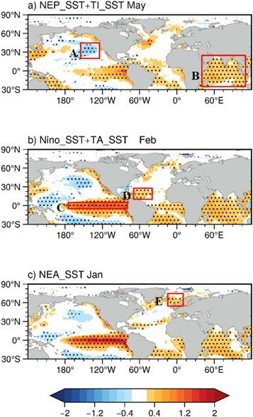
Figure 2. Regression maps of the sea surface temperature (SST) (shading, unit: K) against PC1 for the (a) previous May, (b) previous February and (c) previous January for the period 1980–2009. The dotted regions represent SST anomalies significant at the 90% confidence level. The red boxes denote the regions used to construct the SST indices: (A) NEP_SSTI, (B) TI_SSTI, (C) Nino_SSTI, (D) TA_SSTI and (E) NEA_SSTI.
Download figure:
Standard image High-resolution imageTable 1. Brief descriptions of the selected climate indices used in the present study to build the seasonal forecast models for HWF_EC.
| Index | Description | Location |
|---|---|---|
| NEP_SSTI | Northeastern Pacific Sea Surface Temperature Index | Rectangular region:(125°−155°W, 20°−45°N) |
| TI_SSTI | Tropical Indian Sea Surface Temperature Index | Rectangular region: (40°W-110°E, 25°S-25°N) |
| Nino_SSTI | Nino Sea Surface Temperature Index | Rectangular region: (175°−80°W, 5°S-5°N) |
| TA_SSTI | Tropical Atlantic Sea Surface Temperature Index | Rectangular region: (70°−40°W, 10°−28°N) |
| NEA_SSTI | Northeastern Atlantic Sea Surface Temperature Index | Rectangular region: (15°W-10°E, 55°−75°N) |
| SWA_SMI | Southwestern Asian Soil Moisture Index | Rectangular region: (45°−70°E, 20°−35°N) |
| SEA_SMI | Southeastern Asian Soil Moisture Index | Four endpoints of the rotated rectangular region: (103°E, 12°N), (99°E, 18°N), (118°E, 35°N); (122°E, 30°N) |
| NEA_SMI | Northeastern Asian Soil Moisture Index | Rectangular region: (105°−133°E, 32°−56°N) |
| TP_SCI | Tibetan Plateau Snow Cover Index | Rectangular region: (82°−104°E, 25°−42°N) |
| NA_SCI | Northern American Snow Cover Index | Rectangular region: (90°−125°W, 32°−48°N) |
| Ar_SII | Arctic Sea Ice Index | Three rectangular regions: (180°W-180°E, 82°−90°N); (125°−152°W, 70°−78°N); (120°−150°E, 78°−82°N) |
| NE_SII | Northern European Sea Ice Index | Rectangular region: (30°−44°E, 72°−76°N) |
Table 2. The TCCs between PC1 and the climate indices used in the current study to build the seasonal forecast models for the HWF_EC for the period 1980–2009.
| Index | TCC |
|---|---|
| NEP_SSTI(−1) | 0.49** |
| TI_SSTI(−1) | 0.67** |
| Nino_SSTI(−4) | 0.58** |
| TA_SSTI(−4) | 0.48** |
| NEA_SSTI(−5) | 0.38** |
| SWA_SMI(−4) | 0.41** |
| SEA_SMI(−5) | 0.45** |
| NEA_SMI(−7) | 0.45** |
| TP_SCI(−3) | 0.56** |
| NA_SCI(−4) | 0.35* |
| Ar_SII(−1) | 0.44** |
| NE_SII(−2) | 0.41** |
Note: The TCCs passing the 95% confidence level are marked with '**', while those passing the 90% confidence level are marked with '*'. The climate indices in bold font represent those negatively correlated with PC1. The numbers in the brackets indicate the selected months for the climate indices (for example, NEP_SSTI(−1) means that the month for the NEP_SSTI used in the seasonal forecast model is one month before June-July-August, i.e., May).
Similar to the SST field, three predictors from the soil moisture field (figure 3), i.e., the Southwestern Asian soil moisture (SWA_SMI, table 1) from the previous February (figure 3(a), region 'A'), Southeastern Asian soil moisture (SEA_SMI, table 1) from the previous January (figure 3(b), region 'B') and Northeastern Asian soil moisture (NEA_SMI, table 1) from the previous November (figure 3(c), region 'C'), are chosen as predictors. The lead-lag correlations of these soil moisture predictors to PC1 can be seen in figure 6(b). In addition, two predictors from the snow cover (figure 4) and two predictors from sea ice (figure 5) fields are also selected. In summary, twelve predictors from the lower boundary conditions of the atmosphere from previous periods are selected to construct predictors for the ML models. The specific regions chosen to construct all the constructed SST, SM, SC and SI indices can be found in table 1, and the most significant TCCs between PC1 and the twelve indices are displayed in table 2.
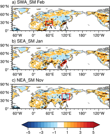
Figure 3. Regression maps of the soil moisture (SM) (unit: %; shading) against PC1 for the (a) previous February, (b) previous January and (c) previous November for the period 1980–2009. The dotted regions represent SM anomalies significant at the 90% confidence level. The red boxes denote the regions used to construct the SM indices: (A) SWA_SMI, (B) SEA_SMI and (C) NEA_SMI.
Download figure:
Standard image High-resolution image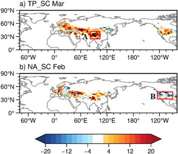
Figure 4. Regression maps of the snow cover (SC) (unit: %; shading) against PC1 for the (a) previous March and (b) previous February for the period 1980–2009. The dotted regions represent SC anomalies significant at the 90% confidence level. The boxes denote the regions used to construct the SC indices: (A) TP_SCI and (B) NA_SCI.
Download figure:
Standard image High-resolution image
Figure 5. Regression maps of sea ice (SI) (unit: %; shading) against PC1 for the (a) previous May and (b) previous April for the period 1980–2009. The dotted regions represent SI anomalies significant at the 90% confidence level. The red boxes denote the regions used to construct the SI indices: (A) Ar_SII (area-averaged SI of all three regions in red boxes) and (B) NE_SII.
Download figure:
Standard image High-resolution image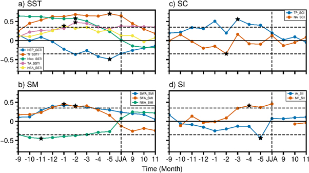
Figure 6. The lead-lag TCCs between PC1 and the (a) SST indices, (b) SM indices, (c) SC indices and (d) SI indices from the previous September (−9) to the following December (11) for the period 1980–2009. 'JJA' on the x axis indicates the simultaneous correlation coefficients of the summer mean between PC1 and the indices. The vertical dashed lines are contemporary labels. The horizontal dashed lines represent the 90% confidence level. The black stars denote the months in which the climate indices are chosen to be potential predictors to build the seasonal forecast models for HWF_EC. The definitions of the indices can be found in table 1.
Download figure:
Standard image High-resolution image5.2. Seasonal forecasts for HWF_EC
To examine the performance of ML models, hindcast experiments are first conducted for PC1 for the period 1980–2009, and a cross-validation scheme is used to verify the model outputs. The hindcasts of PC1 from the two ML models with a take-5-year-out scheme are depicted in figure 7(a) (red and blue lines in figure 7(a) for CatBoost and LightBM, respectively). A linear regression model is utilized to perform the same forecasts for the purpose of a comparison (green line in figure 7(a)). The forecast PC1 from the ML and LR models are highly correlated with those in the observations (black line in figure 7(a)), with all TCCs exceeding 0.65 and significant at the 99% confidence level. The CatBoost model has the highest TCC value of 0.79 for PC1 among all three models.

Figure 7. (a) The normalized PC1 (black) and take-5-year-out hindcast results of the three models, i.e., CatBoost (red), LightGBM (blue) and LR (green). The TCCs between the HWF_EC in the observations and those in the seasonal forecast models of (a) CatBoost, (b) LightGBM and (c) LR for the period 1980–2009.
Download figure:
Standard image High-resolution imageThen, as introduced before, the PC1 from the hindcast experiments and the observational EOF1 are used to construct the forecasting HWF fields according to equation (1). The TCC maps between the observed and forecasted HWF_EC for the two ML and LR modes are depicted in figures 7(b)–(d). A comparison to figures 1(a) and (b) demonstrates that all these models perform reasonably well over the Eurasian continent, especially over regions with high HWF values, i.e., the EUR, SEA and NEA areas. In addition, take-1-year-out and take-10-year-out hindcast experiments are also performed (not shown), and they exhibit similar results to figure 7. The hindcast experiments imply that the two ML models can well forecast the variation of the HWF_EC and have high forecasting skills over areas that usually have frequent heat wave events for the period 1980–2009.
To evaluate the performance of the ML models in predicting the HWF, the ML model predicted and observed PC1 for the period 2010–2019 are compared. The observed PC1 of 2010–2019 is obtained by projecting the observational HWF data for 2010–2019 onto the EOF1 calculated for 1980–2009. Figure 8(a) shows the ML model predicted and observed PC1 during this period. The temporal correlation coefficients (TCCs) of PC1 between the observation and the model prediction are also calculated and presented in figure 8(b). The ML model-predicted PC1 was highly correlated with the observed PC1, with TCCs of 0.73 and 0.82 for CatBoost and LightGBM, respectively, and both passed the 95% confidence level. The TCC for the LR model is 0.61, which is relatively lower than that of the two ML models and cannot pass the 95% confidence level. In addition, the area-weighted-average TCCs of the two ML models and LR model over the Eurasian continent and the regions with high HWF values, i.e., the EUR, SEA and NEA areas, are represented in figure 8(b). The LightGBM models outperform the CatBoost and LR models over the whole Eurasian continent, while they show consistent performance in that both the CatBoost and LightGBM models are superior to LR over the three high HWF regions. In general, the LightGBM model demonstrates higher skills than the CatBoost and LR models, especially over EUR areas, which is consistent with the results shown in figure 8(a).
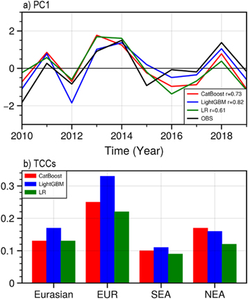
Figure 8. (a) Model-predicted and observed PC1 and (b) Domain-averaged TCCs between the HWF_EC in the observations and those in the seasonal forecast models for the period 2010–2019.
Download figure:
Standard image High-resolution imageThe TCC maps between the observed and forecasted HWF_EC are presented in figures 9(a)–(c). Significant positive TCC skills appear over EUR and NEA areas for the three forecasting models, while the TCC skill for SEA is relatively low. The differences in the TCC skill between the two ML and LR forecasting models are presented in figures 9(d) and (e). Positive values appear over most parts of the Eurasian continent, indicating that the ML models perform better than the LR model during this period. A comparison between the ML models (figure 9(f)) indicates that the LightGBM model obviously outperforms the CatBoost model, especially over EUR and NEA areas.

Figure 9. The TCCs between the HWF_EC in the observations and those in the seasonal forecast models of (a) CatBoost, (b) LightGBM and (c) LR for the period 2010–2019. The dotted regions represent TCCs significant at the 90% confidence level. The differences in TCCs between the CatBoost and LR models are depicted in (d), those between the LightGBM and LR models are depicted in (e), and those between the LightGBM and CatBoost models are depicted in (f).
Download figure:
Standard image High-resolution imageIn seasonal forecasting, it is also important and valuable to know the relative importance of the predictors used in the forecasting models. One advantage of using the two selected ML models in the current work is that they are tree ensemble models and can evaluate the contributions to the seasonal forecasts from each predictor (figure 10). The results for the two ML models vary greatly, indicating that the role of each predictor in the seasonal forecast is model dependent. For example, in the CatBoost model, the NE_SII predictor is the largest contributor, accounting for 14% of the contribution, which is only 5% in the LightGBM model. The TA_SSTI contributes most to the LightGBM model (18%), while it contributes 9% to the CatBoost model. In general, the SST predictors contribute mostly to the seasonal forecasts of HWF_EC, which are 50% and 43% for the CatBoost and LightGBM models, respectively. For the LightGBM model, which performs the best among the three forecasting models, the tropical Atlantic SST (TA_SSTI) and the Northeastern Asia soil moisture (NEA_SMI) contribute mostly to the forecast (18% and 16%, respectively) compared to other predictors.
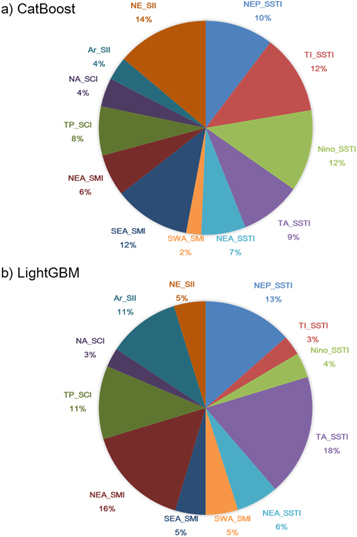
Figure 10. The contribution of each predictor (unit: %) to the seasonal forecasts of PC1 in the model forecasts of (a) CatBoost and (b) LightGBM.
Download figure:
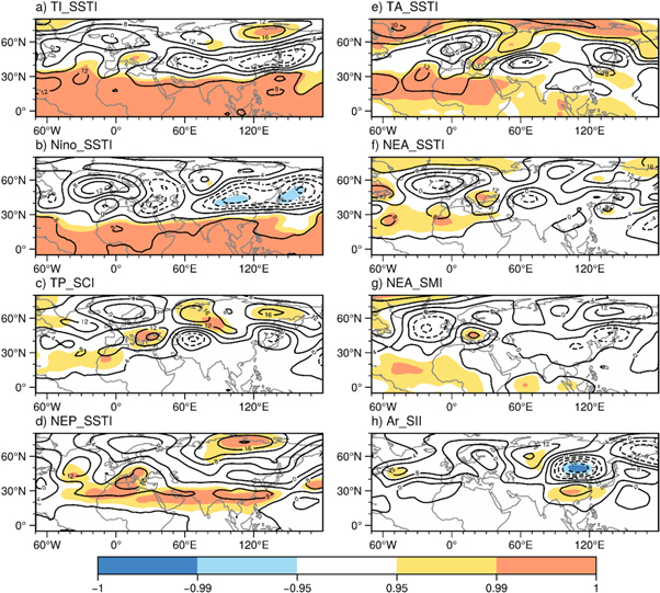
Standard image High-resolution imageAs we mentioned before, HWF_EC displays continental-scale patterns and is impacted by large-scale atmospheric circulation anomalies. The Z200 anomalies associated with the eight climate indices, which have most high TCC skills between PC1(table 2), are obtained by regression (figure 11). Significant and different Z200 anomalies associated with these predictors appear over the Northern Hemisphere, indicating that these climate predictors may contribute to the HWF_EC by modulating large-scale atmospheric circulations. Although there were obvious differences in the spatial distributions, as shown in figure 11, high-pressure anomalies could be noticed over the three large HWF regions. However, further research on the dynamic mechanisms accounting for how climate predictors impact summer HWF_EC is worth examining in the future using both observational data and numerical models. According to figure 10, focus can be given to explore the possible mechanism of how the tropical Atlantic SST and the Northeastern Asia soil impact the HWF_EC in future studies.
Figure 11. The anomalies of the 200 hPa geopotential height (Z200; unit: Pa, contours) regressed against the (a) TI_SSTI, (b) Nino_SSTI, (c) TP_SCI, (d) NEP_SSTI, (e) TA_SSTI, (f) NEA_SSTI, (g) NEA_SMI and (h) Ar_SII with the corresponding confidence level (shading) for the period 1980–2009.
Download figure:
Standard image High-resolution image
6. Discussion and conclusions
It is known that current climate models usually perform poorly in forecasting heat wave events. Compared to traditional analysis methods, ML methods can capture the complex nonlinear relationship between the predictor and predictand and therefore may provide an additional and useful tool for seasonal forecasting. In addition, some tree ensemble ML models can evaluate the relative importance of each predictor, which provides more valuable information to the seasonal forecasts than traditional regression models.
In this work, we identified a continental-scale summer HWF pattern over the Eurasian continent (HWF_EC) for the period 1980–2019, with three large HWF areas lying over EUR, SEA and NEA. Two ML models are used to perform seasonal forecasts for the summer HWF_EC. An LR model is also utilized to perform parallel forecasts for the purpose of comparison. The potential predictive sources for the summer HWF_EC, i.e., SST, SC, SM and SI, are chosen through the lower boundary conditions of the atmosphere using lead-lag correlation analysis. Predictors for seasonally forecasting the summer HWF_EC are constructed by averaging the lower boundary conditional fields in regions at the month that are persistently and most significantly correlated with the temporal variation of EOF1 of HWF_EC. Both the hindcast and real seasonal forecast experiments are performed for the summer HWF_EC.
In the hindcast experiments for the period 1980–2009, the ML models can well predict the variation of the HWF_EC and show high TCC skills over all three large HWF regions. In the real forecast of 2010–2019, the ML models perform well over EUR and NEA but have relatively low forecast skill over SEA. The two ML models show higher forecast skills than the LR model, and the LightGBM model obviously outperforms the CatBoost model. An analysis of the contribution from each predictor to the ML model forecasts shows that the relative importance of the predictor to the seasonal forecasts is model dependent. The predictors of the tropical Atlantic SST and the Northeastern Asia soil play the most important roles in the LightGBM model. In general, the five SST predictors together account for almost half of the contributions to the seasonal forecast for HWF_EC.
Acknowledgments
This research is funded by the National Natural Science Foundation of China (grant 42075050).
Appendix
A.1. GBDT
The gradient boosting decision tree (GBDT) is one type of ML technique called gradient boosting that gives an integrated prediction model in the form of an ensemble of weak prediction models (Friedman, 2001). The weak learners, i.e., prediction models in GBDT, are decision trees (DTs). It is a supervised ML model that can be used in regression and classification tasks. DTs split the tree node by evaluating the error observed in each tree node through a loss function. The GBDT model is an iterative algorithm in which new DTs are added based on the residual produced by previous DTs during the iterations to continuously improve the overall accuracy of the integrated model. More details on the computation processes are described in Friedman (2001).
Since the model is based on DTs, the relative contribution of each predictor can be evaluated (Brieman et al (1984). When a predictor is used to split a tree node, its importance can be estimated by calculating the improvement of model accuracy in a single tree. For the whole GBDT model, the contribution is the average importance of all the additive trees.
A.2. LightGBM
The LightGBM model is based on GBDT and was proposed by Ke et al (2017) to address dissatisfactions about the efficiency and scalability of GBDT when confronting large feature dimensions or data sizes. All data instances need to be scanned to estimate the information gain of all possible segmentation points in GBDT models, which leads to large computing expenses. Two novel techniques, gradient-based one-side sampling (GOSS) and exclusive feature bundling (EFB), are applied to address this problem in the LightGBM model. Through GOSS, a significant proportion of data instances with small gradients can be excluded. It is proven that only using data instances with larger gradients can obtain quite accurate estimations of the information gain. Mutually exclusive features are bundled to reduce the number of feature dimensions with EFB. The LightGBM model can speed up the training process and obtain almost the same accuracy as conventional GBDT. More detailed information can be found in Ke et al (2017).
A.3. CatBoost
CatBoost is another GBDT-based ML mode, which is based on oblivious trees with fewer parameters and handles categorical features more effectively than standard GBDT models (Dorogush et al 2018). In CatBoost, categorical features, which have a discrete set of values, are not necessary to substitute numerical values at the preprocessing phase. The CatBoost model provides several methods to deal with categorical features and conducts feature combinations to fit the optimal models. Apart from the advantages of this algorithm in handling categorical features, another advantage is its new schema for calculating leaf values when selecting the tree structure, which reduces overfitting. Detailed analysis of the algorithm refers to Prokhorenkova et al (2018).