

Abstract
Understanding the dynamics of water-energy-food (WEF) nexus interactions with climate change and human intervention helps inform policymaking. This study demonstrates the WEF nexus behavior under ensembles of climate change, transboundary inflows, and policy options, and evaluates the overall nexus performance using a previously developed system dynamics-based WEF nexus model—WEF-Sask. The climate scenarios include a baseline (1986–2014) and near-future climate projections (2021–2050). The approach is demonstrated through the case study of Saskatchewan, Canada. Results show that rising temperature with increased rainfall likely maintains reliable food and feed production. The climate scenarios characterized by a combination of moderate temperature increase and slightly less rainfall or higher temperature increase with slightly higher rainfall are easier to adapt to by irrigation expansion. However, such expansion uses a large amount of water resulting in reduced hydropower production. In contrast, higher temperature, combined with less rainfall, such as SSP370 (+2.4 °C, −6 mm), is difficult to adapt to by irrigation expansion. Renewable energy expansion, the most effective climate change mitigation option in Saskatchewan, leads to the best nexus performance during 2021–2050, reducing total water demand, groundwater demand, greenhouse gas (GHG) emissions, and potentially increasing water available for food&feed production. In this study, we recommend and use food&feed and power production targets and provide an approach to assessing the impacts of hydroclimate and policy options on the WEF nexus, along with suggestions for adapting the agriculture and energy sectors to climate change.
Export citation and abstract BibTeX RIS

Original content from this work may be used under the terms of the Creative Commons Attribution 4.0 licence. Any further distribution of this work must maintain attribution to the author(s) and the title of the work, journal citation and DOI.
1. Introduction
The basic life-supporting pillars—water, energy, and food (WEF) are exposed to climate change, leading to uncertainty in WEF security and challenges to policymaking. This situation becomes more complex when the dynamics of WEF systems are poorly understood (Wu et al 2021). Moreover, given the strong interrelations among WEF sectors, resource management without coordination may lead to unintended consequences. Naturally, a 'nexus' thinking has been widely accepted and increasingly valued by researchers (Hoff 2011, Scanlon et al 2017, Liu et al 2017, Huntington et al 2021).
Given the far-reaching influence of climate variability on natural and human systems, mitigation and adaptation strategies are usually presented to slow down the rate of climate change or improve the resilience of vulnerable systems. These strategies often result in trade-offs or synergies. He et al (2019) demonstrated that the extended use of wind and solar power effectively reduces water consumption and competition over it, avoiding the over-exploitation of groundwater in California, USA. Biofuel use in transportation is another hotspot for carbon mitigation by blending gasoline with ethanol or diesel with biodiesel. However, this policy has been controversial, in part due to the competitive use of water and land for food or biofuel production. Furthermore, intensive diversion of grains to biofuel production is likely to increase grain prices, leading to negative impacts on food consumers and livestock farmers (Bhullar et al 2012). Large irrigation expansion often competes for water with hydropower plants as follows: in multipurpose reservoirs, more water tends to be stored to achieve a higher hydraulic head, even during dry seasons, for hydropower generation, while downstream farmers need timely water released to irrigate crops in the growing season (He et al 2019). A declined hydropower production hampers the efforts of the transition from fossil fuels to renewables, which is increasingly favored by current energy policies.
Investigating the WEF nexus and its interactions with human interventions is usually complicated by the compounding effect of uncertain climate change and variability, and relevant studies are insufficient. Yang et al (2016) distinguished the 'acceptable' and 'unacceptable' scenarios considering crop and hydropower production and flood-affected area in the Brahmaputra River Basin, a transboundary river basin in South Asia, under changes of precipitation, temperature, and water diversions from upstream countries. However, they only discussed conflicting benefits in the water resources system while not explicitly addressing the co-benefits or synergies, which are often identified on the basis of comprehensive water, energy, and food links. Additionally, simply changing temperature and precipitation by intervals, as conducted by Yang et al (2016), ignores the inter-dependence between them. Lee et al (2020) analyzed a food-centric WEF nexus in paddy rice production under climate projections and different irrigation methods (continuous irrigation versus intermittent irrigation) using the footprint concept as linkage indicators, such as water footprint (m3/ton), energy footprint (GJ/ton), and land footprint (ha/ton). However, the discussion of the WEF nexus was limited to paddy rice production without considering the direct, broad, and profound consequences for water resources or the energy sector. Moreover, a few deterministic projections of climate scenarios convey limited information and often ignore the internal (stochastic) weather variability, probably limiting the validity of the study conclusions. Abdelkader et al (2018) explored the national water, food, and trade in Egypt. Further, Abdelkader and Elshorbagy (2021) investigated and identified robust solutions under varying climate conditions in Egypt, linking national water management to the global food trade. However, these two studies were limited only to the water-food nexus. Few studies explored issues along transboundary rivers from a nexus viewpoint in North America. Zhang et al (2021) explored the human dimension of the food-energy-water-environment (FEWE) nexus in the Columbia River basin between the US and Canada by conducting a workshop and a survey.
Generally, the dynamics of how the WEF nexus interacts with climate change and policy options remain poorly understood. From practical and policy viewpoints, assessing the impact of climate and policy on WEF nexus needs to be referenced against targets, e.g., food, energy, or environmental targets, for objective and quantitative evaluation, which is rarely explored. This study provides an approach to exploring the impacts of climate change and policy options on the WEF nexus at a provincial scale. Specifically, this study demonstrates thousands of potential future pathways of WEF nexus, projected based on combinations of future climate signals, internal weather variability, transboundary inflows, and policy options of food&feed and energy sectors. In contrast to some existing WEF nexus studies dealing with climate change impacts, this study considers different climate change signals from the total available 85 combinations of GCMs and SSPs. Direct impacts of climate change on various sectors (e.g., irrigation, energy demand, streamflow) and indirect nexus effects are evaluated. Furthermore, we present WEF nexus behavior, identifying desired and undesired scenarios for individual sectors and the whole nexus. While doing this, we show the impact of policies (e.g., renewable energy and irrigation expansion) on the WEF nexus under ensembles of climate and hydrological scenarios for a case study in Saskatchewan, Canada.
2. Case study
Saskatchewan is one of the prairie provinces in western Canada, covering an area of 651,036 km2, with latitude from 49°N to 60°N and longitude from 110 °W to 102°W (Lewry and Ward 2021; figure 1). The province's economy depends on agriculture and natural resources. Saskatchewan has 18.9 million hectares of cultivated farmland, 99.2% of which are rainfed (Government of Saskatchewan 2020). Agricultural activities are concentrated in the southern half of the province, a semi-arid area with annual precipitation of 319–415 mm and annual mean temperature of 0.6 °C–3.9 °C (Climate Atlas of Canada 2019), but scattered over eight large basins (figure 1). Although irrigated area accounts only for 0.8% of the total cultivated farmland, irrigation is the largest water consumer with an average annual water withdrawal of 231.4 million m3 during 2006–2017, accounting for 45.7% of total water use in Saskatchewan (Government of Saskatchewan 2019a). Centre pivots are the most common irrigation system, and the most common conveyance methods are either combined canal and pipelines or direct pipelines from reservoirs/rivers to farms. Water use efficiency increases by lining canals and pipelines replacing canal systems (Government of Saskatchewan 2019b, Saskatchewan Water Security Agency 2021). In addition, Saskatchewan centre pivot design and construction commonly use electricity for driving the wheels and pumping water (Government of Saskatchewan 2012, Government of Saskatchewan 2019b). The boom in agriculture makes Saskatchewan the world's largest exporter of peas, lentils, durum wheat, mustard seed, and canola (Government of Saskatchewan 2019c). Figure 2 shows food and feed production and harvested area by crop in 1986–2016.
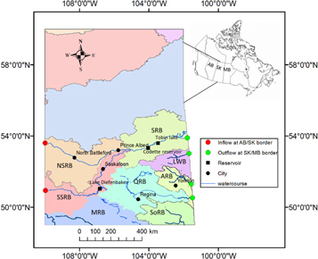
Figure 1. Map of the location of Alberta/Saskatchewan border flows, reservoirs, and cities in the river basins in South Saskatchewan. SSRB—South Saskatchewan River Basin, NSRB—North Saskatchewan River Basin, SRB—Saskatchewan River Basin, ARB—Assiniboine River Basin, MRB—Missouris River Basin, QRB—Qu'Appelle River Basin, SoRB—Souris River Basin, LWB—Lake Winnipegosis Basin. AB—Alberta, SK—Saskatchewan, MB—Manitoba.
Download figure:
Standard image High-resolution image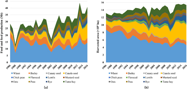
Figure 2. Major food and feed production in million tonnes (Mt) and harvested area in hectare (ha) in Saskatchewan (Source: Statistics Canada (2021)).
Download figure:
Standard image High-resolution imageLake Diefenbaker provides water in Saskatchewan for 60% of the province's population, major irrigation areas, hydropower generation, industries, mining, and aquaculture (Saskatchewan Water Security Agency 2012). Large irrigation expansion, currently underway in the Lake Diefenbaker area (figure 1), will increase water withdrawal and might intensify water competition with other sectors, such as the municipalities, energy, and other industries. This policy may exacerbate pressure on freshwater resources, particularly under the unprecedented rapid growth of population and economic development, and climate change (Saskatchewan Water Security Agency 2012). The key water sources for irrigation and hydropower production are transboundary (inter-provincial) rivers—the South Saskatchewan River (SSR) and the North Saskatchewan River (NSR), which start from the Rocky Mountains in the upstream province of Alberta. The transboundary flows are managed by the 1969 Master Agreement on Apportionment that requests Alberta to pass 50% of the natural flow to Saskatchewan, which also needs to pass 50% of the flow delivered from Alberta as well as local natural flows to the downstream province of Manitoba (Prairie Province Water Board 2015). Groundwater is another essential water source that supports 75% of communities or 43% of the population for drinking (Saskatchewan Water Security Agency 2012, Government of Canada 2013). In 2018, Saskatchewan produced 24.3TWh of electricity (Canada Energy Regulator 2021): about 84% from fossil fuels (44% from natural gas, 40% from coal) and 16% from renewables (14% from hydroelectricity, 2% from wind power). In response to climate change, Saskatchewan has policies and developed plans to expand renewable energy production (e.g., wind/solar power) and consumption (e.g., ethanol and biodiesel in transportation). For example, Saskatchewan plans to expand its wind capacity to 30% of total power capacity by 2030 (Saskatchewan Chamber of Commerce 2019).
3. Methodology
The overall methodology consists of the following steps: (1) Four different near-future climate scenarios (2021–2050) were selected out of 85 separate projections based on 21 GCMs from CMIP6 (table S1 (available online at stacks.iop.org/ERC/4/015009/mmedia)). Additionally, the baseline climate scenario reflecting no change in the statistics of historical (1986–2014) climate variables was also used; (2) a stochastic weather generator (LARS-WG) was used as a downscaling tool to generate daily-scale 100 realizations of each climate change scenario and baseline in each basin; (3) 500 stochastically generated transboundary inflow series to Saskatchewan, through both SSR and NSR, were utilized based on the approach of Nazemi et al (2013). The generated transboundary flows cover a range of −20% to 20% (in 10% increments) of the 31-year average annual flow (1980–2010); (4) WEF-Sask model was used to capture the WEF nexus driven by socioeconomic and climatic variables and surface water flows. The local flows in each basin were simulated by a prairie watershed model (HYPR, Ahmed Mohamed et al 2020) using the downscaled climate scenarios; (5) Three policy options were considered as potential human interventions as detailed in section 3.3. In total, the WEF-Sask model can be driven by the 750,000 combinations (5 transboundary flow signals × 100 stochastic flow realizations × 5 climate signals × 100 stochastic climate realizations × 3 policy options). However, this was reduced to 7,500 runs considering the computational budget (1.5 minutes for one run on processor—Intel(R) Core(TM) i7–7700 CPU @ 3.60 GHz, 16 GB RAM). The detailed information on how to select the 7,500 runs was described in section 3.3. Food&feed and hydropower production targets were also set to distinguish the desired and undesired scenarios. Specifically, the annual primary food&feed production target is 31.8 million tonnes (Mt), which is assumed 8% higher than historical long-term average values (1986–2016), considering the effects of increased nutrient application on agricultural production (McKenzie et al 2003). The annual hydropower production target was assumed as 3.65 TWh, which is the simulated average value during 1986–2016. Details of the methodology are provided in the following three sub-sections.
3.1. Climate change scenarios
In this study, the historical period (1986–2014) was considered as the baseline and 2021–2050 as the near-future period in climate scenarios. Climate change projections were based on the Coupled Model Intercomparison Project Phase 6 (CMIP6). The daily precipitation (pr), daily minimum temperature (Tmin), daily maximum temperature (Tmax), monthly solar radiation (shortwave incoming radiation; rad), monthly wind speed (ws), monthly surface pressure (sp), and monthly specific humidity (hum) datasets, provided by the available 21 Global Climate Models (GCMs) for the baseline and near-future periods, were acquired from https://esgf-node.llnl.gov/search/cmip6/. The CMIP6 provides climate change projections using a wide range of forcings as the GCMs included in CMIP6 consider Shared Socioeconomic Pathways (SSPs) (Eyring et al 2016, Stouffer et al 2017). Table S1 (available online at stacks.iop.org/ERC/4/015009/mmedia) shows the list of CMIP6 GCMs, climate modeling centers, and SSPs.
A total of 85 climate scenarios (table S1 (available online at stacks.iop.org/ERC/4/015009/mmedia)) were available based on the combinations of GCMs and SSPs, and the k-means clustering method (section S2) was used to identify a small set of scenarios with climate signals across the range of the 85 separate projections, many of which have similar climate signals. Future projections of climate change can be differentiated based on the monthly relative change factors (RCFs, Semenov and Barrow, 2002). The RCFs were calculated for each of the 85 scenarios using six different monthly statistics (mean monthly values of precipitation, wet spell length, dry spell length, Tmin, Tmax, and standard deviation of daily mean temperature) for each of the 12 months, which resulted in 72 RCFs (figure S2 (available online at stacks.iop.org/ERC/4/015009/mmedia)). These RCFs quantify the relative change of the future climate signal (2021–2050) of a scenario relative to the baseline (1986–2014). Four clusters (k = 4) were selected based on the analysis described in section S2, and the climate scenarios close to the cluster centers were picked as representatives of the range of climate possibilities (figure S1 (available online at stacks.iop.org/ERC/4/015009/mmedia)): MIROC6-ssp126, HadGEM3-GC31-LL-ssp245, UKESM1–0-LL-ssp370, and FGOALS-g3-ssp585. Interestingly, the selected scenarios combine representatives of four different GCMs (the British HadGEM3 and UKESM, the Chinese FGOALS, and the Japanese MIROC6), four SSPs (1, 2, 3, and 5), and for radiative forcings (2.6, 4.5, 7.0, and 8.5 Wm−2 by 2100).
A user-friendly and widely used stochastic weather generator, Long Ashton Research Station Weather Generator LARS-WG (Semenov and Barrow 2002), was used to downscale climate variables from the global scale to the local scale (centroid of each river basin). First, LARS-WG 5.5 was used to construct probability distributions of climate variables for the baseline period using the historical gridded (0.5 × 0.5°) climate data from the WFDEI (Weedon et al 2014). The baseline probability distributions were used to generate 100 realizations of each climate variable with a length of 30 years based on the historical climate records from the 1986–2014 period, and the statistics of the realizations were compared to the statistics of the historical climate data (figure S3 (available online at stacks.iop.org/ERC/4/015009/mmedia)) to validate the use of LARS-WG in our study area. Although LARS-WG 5.5 did not facilitate downscaling of surface pressure, wind speed, and specific humidity, solar radiation was used as the dummy variable for these three variables. This was achieved by scaling other variables to match the range of solar radiation and rescaling back to match their actual range after downscaling was completed. The performance of this approach is shown in (figure S3 (available online at stacks.iop.org/ERC/4/015009/mmedia)). Second, the calculated monthly RCFs for each climate variable were used to perturb the parameters (e.g., mean, standard deviation) of the baseline probability distributions. Finally, the perturbed probability distributions were used to generate 100 realizations of the seven climate variables for the four future climate scenarios (2021–2050).
3.2. Modeling framework
WEF-Sask is an integrated model that incorporates the production/supply and demand sides of the water, energy, and food&feed sectors in Saskatchewan at the provincial scale using the system dynamics approach (Wu et al 2021). Crop yield was modeled based on physical processes, and crop production is the product of crop yield and cropland. Food or feed demand (except crops for bioenergy) was simply estimated based on per capita demand and population or animal heads. Energy demand by end-uses (e.g., electricity, natural gas, gasoline, biodiesel) in different sectors (residential, industry, transportation, commercial) was estimated using simple inductive models based on regression relationships. The predictors among the equations include GDP, population, heating degree days (HDD), cooling degree days (CDD), and natural gas price. Agricultural energy consumption (except energy demand for irrigation water supply) was estimated based on energy input coefficient (e.g., MJ/ha, kWh/head) and cropland area or livestock population. Electricity required for irrigation water supply was calculated based on irrigation water volume, total pressure head needed to pump and apply water, and pump and motor efficiency. Bioenergy demand was estimated based on the blending mandate (e.g., 25% ethanol, 11% biodiesel) and total gasoline and diesel demand in the transportation sector. Since the blending mandate fraction is known, biofuel demand can be calculated. Further, demand for bioenergy feedstock—wheat for ethanol and canola seed for biodiesel in Saskatchewan (Hayes and Bradford 2019) was estimated in the model by converting bioenergy demand to feedstocks demand. Electricity production (coal-fired, natural gas-fired, and wind power as well as hydropower) was assumed to always meet electricity demand because of the negligible net import in the historical records. The details in modeling water, energy, and food sectors as well as their interactions, are described by Wu et al (2021). In general, the WEF-Sask comprehensively models interconnections between water, energy, and food, highlighting the trade-offs and synergies. Furthermore, it connects the WEF systems to socioeconomic and climatic drivers and conveniently investigates the impacts of mitigation and adaptation strategies on the WEF nexus. Therefore, integrated with large ensembles of potential future conditions, the WEF-Sask model allows for examining the interactive dynamics of the WEF systems and drivers and demonstrates the trajectories of the WEF nexus. In this study, indicators including total water demand (TWD), groundwater demand (GWD), transboundary water transferred to Manitoba (WTMN), food and feed production (FP), food surplus (FP), hydropower production (HP), thermal power production (ThP), and greenhouse gas emissions (GHG), were reported to evaluate the overall WEF nexus performance. The model runs at a daily scale, and the results can be flexibly reported on other scales, e.g., monthly or annual. The water resource component of the original WEF-Sask model simulates the existing surface water system using measured streamflow. To project surface water system under climate scenarios, HYdrological model for Prairie Region (HYPR) (Ahmed Mohamed et al 2020), developed specifically for the Canadian prairies to capture the challenging pothole dynamics, was used to generate local flows. Variability of the transboundary inflows was also considered with the WEF-Sask model, and it is briefly explained in the following section. Groundwater is required in oil and natural gas production (Wu et al 2021) and was also assumed to supplement surface water shortfalls in the municipal, livestock, and industrial sectors in this study. Since almost all irrigation water use is from surface water supplies (only 0–0.23% or 0–0.45 million cubic meters of irrigation water is supplied by groundwater in 2012–2017) (personal communication), we ignored the groundwater as a water source for irrigation in the future.
3.3. Experimental setup
Three policies were designed to be investigated in combination with the ensemble climatic and transboundary flow scenarios:
- Maintaining the current power mix (CP) ratios: The ratios of coal-fired, natural gas-fired, and wind power, as well as hydropower, maintain the current level. Given that hydropower production fluctuates, we assumed that renewable energy first meets electricity demand, followed by thermal power.
- Renewable energy expansion (RE) policy: A proposed future power mix (coal-fired, natural gas-fired, and wind power as well as hydropower) was used to limit carbon emissions (table 1; Canada Energy Regulator 2020) while other conditions maintain the same level as CP.
- Renewable energy and irrigation expansion (REI) policy: Both the energy and food policies were assumed to be implemented simultaneously. The irrigation expansion is already at the pre-feasibility study stage that provides information for an in-depth design and construction in Saskatchewan. The impacts of irrigation expansion can be analyzed by comparing the results of REI and RE experiments.
Table 1 shows the socioeconomic, climatic, and hydrological scenarios under the three policies: CP, RE, and REI. Inputs include five climate scenarios (Baseline, SSP126, SSP245, SSP370, SSP585), five transboundary inflow changes (−20%, −10%, 0, 10%, 20%), and three policies. Given the possible large fluctuations of future natural flow that is supposed to pass from Alberta to Saskatchewan according to the interprovincial water apportionment agreement and uncertain water demand in Alberta, accounting for projected transboundary flows entering Saskatchewan is quite challenging. Instead, we adopted a stochastic approach developed by Nazemi et al (2013), considering the climate impact on streamflow (Pomeroy et al 2009). The sequence number (from 1 to 100) of 100 realizations of a climate signal corresponds to the same sequence number (from 1 to 100) of 100 realizations of a transboundary flow signal. Therefore, 100 runs are selected from 100 × 100 pairwise combinations for each combined climate signal and transboundary flow signal to save the computational budget. Therefore, we ended up with 5 (climate scenarios)×5 (transboundary inflow scenarios) × 100 (stochastic realizations) × 3 (policy options) = 7,500 runs in total. In the food&feed sector, 12 rainfed crops (wheat, barley, oats, flaxseed, rye, canola, chickpeas, lentils, peas, tame hay, canary seed, mustard seed) and 8 irrigated crops (wheat, barley, flaxseed, canola, potatoes, peas, tame hay, corn silage) were simulated. Considering the most used centre pivots system and increasing water use efficiency through lined canals and pipelines, 0.8 was assumed as irrigation application efficiency (Irmak et al 2011) while conveyance efficiency was assumed as 0.9 (Fader et al 2016). Therefore, the overall irrigation efficiency was set to 0.72. Additionally, 11 major export crops (wheat, barley, oats, chickpeas, lentils, peas, canola, flaxseed, rye, canary seed, mustard seed) were selected to estimate food surplus (production minus local consumption; Wu et al 2021), which represents food export potential.
Table 1. Future socioeconomic, climate, and hydrological scenarios during 2021–2050 under three policies. CP—current power mix, RE—renewable energy expansion. REI—renewable energy and irrigation expansion.
| Policy | |||||
|---|---|---|---|---|---|
| Social-economic, Climatic, and hydrological inputs | CP | RE | REI | References | |
| Population annual growth rate (%) | 1 | 1 | 1 | Canada Energy Regulator (2020) | |
| GDP annual growth rate (%) | 1 | 1 | 1 | Canada Energy Regulator (2020) | |
| Natural gas production | — | — | — | Canada Energy Regulator (2020) | |
| Crude oil production | — | — | — | Canada Energy Regulator (2020) | |
| Wind power proportion (%) | 2 | 43 | 43 | Canada Energy Regulator (2020) | |
| Coal-fired power ratio to thermal power (%) | 48 | 9 | 9 | Canada Energy Regulator (2020) | |
| Natural gas-fired power ratio to thermal power (%) | 52 | 91 | 91 | Canada Energy Regulator (2020) | |
| Animal annual growth rate (%) | Cattle and buffaloes | 0 | 0 | 0 | Alexandratos (2012) |
| Sheep and goat | 0.4 | 0.4 | 0.4 | ||
| Pigs | 0.1 | 0.1 | 0.1 | ||
| Poultry | 0.7 | 0.7 | 0.7 | ||
| Irrigated area in Lake Diefenbaker area (ha) | 50,000 | 50,000 | 250,000 | Saskatchewan Water Security Agency (2012) | |
| Ethanol blending rate (%) | 0 | 25 | 25 | Natural Resources Canada (2018) | |
| Bio-diesel blending rate (%) | 0 | 11 | 11 | Canadian Canola Growers Association (2021) | |
| Climate scenarios | Baseline | Baseline | Baseline | https://esgf-node.llnl.gov/search/cmip6/ | |
| SSP126 | SSP126 | SSP126 | |||
| SSP245 | SSP245 | SSP245 | |||
| SSP370 | SSP370 | SSP370 | |||
| SSP585 | SSP585 | SSP585 | |||
| Transboundary inflow change (%) | −20 | −20 | −20 | Nazemi et al (2013), Hassanzadeh et al (2016) | |
| −10 | −10 | −10 | |||
| 0 | 0 | 0 | |||
| 10 | 10 | 10 | |||
| 20 | 20 | 20 | |||
Note: Wheat and canola seed are two major feedstocks for ethanol and biodiesel, respectively (Hayes and Bradford 2019).
4. Results and discussion
This section describes the impacts of climate change and policy options on the WEF nexus. Climate change drives both the demand and production/supply sides of the local water, energy, and food&feed sectors. In addition, possible transboundary inflow changes (Nazemi et al 2013), based on climate change effects (Martz et al 2007), were used to drive the nexus system. Table 2 and figure S4 (available online at stacks.iop.org/ERC/4/015009/mmedia) demonstrate the statistics of the baseline (1986–2014) and projected near-future periods (2021–2050) for the main influential climate variables—precipitation and temperature, in Saskatchewan. SSPs126, 245, 370, and 585 correspond to the radiative forcings 2.6, 4.5, 7.0, and 8.5 Wm−2 by 2100, respectively. Higher radiative forcings are often associated with higher temperature in the far future (Eyring et al 2016), however, this relationship is not always the same in the near future. For example, radiative forcing 8.5 Wm−2 by 2100 could have a lower temperature than other radiative forcings in the near future (before 2050) while obviously higher temperature than other radiative forcings in the far future (∼2100) (Alam et al 2018). Furthermore, the effects of three policy options, including (i) current power mix (CP), (ii) renewable energy expansion (RE), and (iii) combined renewable energy and irrigation expansion (REI), were evaluated.
Table 2. Average daily temperature and cumulative rainfall during the growing season (May to September) for the Baseline (1986–2014) and four GCM scenarios (2021–2050). Tmean is the average value of Tmax and Tmin. The weather variables are the average values of the eight basins in Saskatchewan.
| Baseline | MIROC6-ssp126 | HadGEM3-GC31-LL-ssp245 | UKESM1-0-LL-ssp370 | FGOALS-g3-ssp585 | |
|---|---|---|---|---|---|
| Tmax (°C) | 22.18 | 24.07 | 25.17 | 24.80 | 23.24 |
| Tmin (°C) | 8.35 | 9.61 | 10.72 | 10.48 | 9.46 |
| Tmean (°C) | 15.26 | 16.84 | 17.95 | 17.64 | 16.35 |
| Rainfall (mm) | 296 | 289 | 303 | 290 | 317 |
4.1. Nexus perspective of the impacts of hydroclimate and policy options on WEF related indicators
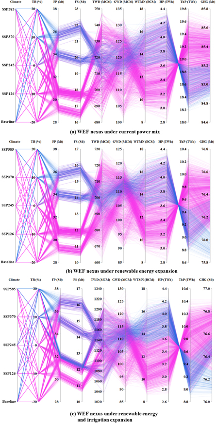
Figure 3 demonstrates the changes of sample indicators (revealing the important interactions among water, energy, and food) under various hydroclimatic scenarios and policy options compared to the baseline scenario. Reflecting the 'business as usual', the baseline scenario majorly assumes the recent trends of growth rates in population and GDP, current irrigated area, and current power mix (table 1, socioeconomic inputs under 'CP' column), combined with baseline climate and no change in transboundary inflows (TB = 0%). The baseline scenario can be used as a reference to evaluate the impacts of changes in climate and policy options. Figure 3(a) shows that climate change can increase or decrease total water demand under the CP policy option due to the mixed effects of climate change on water demand for irrigation which is the largest water user. Warmer temperature can increase reference evapotranspiration (ETo) rate but also accelerate crop growth rate and shorten the growing period. Therefore, crop water demand may either increase or decrease under rising temperatures during the growing season (Hopmans and Maurer 2008). Additionally, climate scenarios with higher rainfall amounts during the growing season allow crops to use more soil water, and thus, less blue water is needed for irrigation. For example, SSP126 (+1.6 °C, −7 mm) increases irrigation water demand by 4.5%, while SSP245 (+2.7 °C, +7 mm) reduces irrigation water demand by 6.8% (figure 3(b)). Renewable energy expansion reduces water demand for thermal power cooling and, therefore, reduces total water demand by 0.1%-5.4% across various climate scenarios (figure 3(a)). Irrigation expansion from 50,000 to 250,000 ha in the Lake Diefenbaker area increases irrigation water demand by 112%–144% across various climate scenarios. Under the combined effect of climate change, renewable energy expansion, and irrigation expansion, total water demand increases by 50%–65% (figure 3(a)).

Figure 3. Percentage change in total water demand, irrigation water demand, total food and feed production, irrigated food and feed production, hydropower production, and GHG emissions (30-year averaged annual values) under hydroclimatic scenarios and policy options during 2021–2050 compared to the baseline scenario. Bars show the percentage change of the average value of 100 realizations.
Download figure:
Standard image High-resolution imageFigure 3(c) shows that all climate change scenarios (SSPs 126, 245, 370, 585) reduce total food and feed production. For instance, SSP370 (+2.4 °C, −6 mm) reduces total crop production by 18% under CP and RE and 15% under REI due to higher temperature and less rainfall. SSP245 (+2.7 °C, +7 mm) has the same effects on total crop production as SSP126 (+1.6 °C, −7 mm) due to the compensating effect of higher rainfall for the higher temperature, and both lead to a 14% reduction in total crop production. However, SSP245 reduces more irrigated crop production (−13% under CP and −7% under RE) than SSP126 (−11% under CP and −5% under RE) because rainfall is not a limiting factor (soil water deficit can be met by irrigation) and crop production is predominantly affected by temperature (figure 3(d)). Renewable energy expansion (RE) has slight synergistic benefits to food and feed production: compensating for the loss of irrigated crop production due to climate change because water saved from thermal power cooling can be translated into higher yields in the irrigated area that depends on unreliable local flows. Although irrigation expansion enhances total food and feed production by 3.2% under Baseline climate due to the benefits to irrigated crop production (increasing by 138%–175%; figure 3(d)), this benefit is fully offset by climate change in the scope of total crop production.
Figure 3(e) shows hydropower production under hydroclimatic conditions and policy options. Renewable energy expansion does not affect hydropower production because transboundary rivers provide reliable and sufficient water if no large irrigation expansion occurs. As expected, the transboundary flow changes mainly affect hydropower production. For example, under CP or RE policy options, a 20% decrease in transboundary flows (TB = −20%) reduces hydropower production by 12.7%–13.2%, while a 20% increase in transboundary flows (TB = 20%) increases hydropower production by 13.5%–14.0% under various climate scenarios. Irrigation expansion reduces hydropower production by 3.2% compared to CP or RE under all hydroclimatic conditions. Thus, irrigation expansion should be carefully managed considering uncertain climate and water supply and externalities to other stakeholders such as hydropower production. Figure 3(f) shows that GHG emissions slightly decrease as transboundary flows increase when adopting the CP policy option. The reason is that higher hydropower production resulting from increased transboundary flows leads to less thermal power production and, therefore, less GHG emissions. Renewable energy expansion effectively reduces GHG emissions by 10.5% on average because additional wind power expansion and expanded biofuel use in transportation directly cut GHG emissions. Irrigation expansion slightly offset these benefits by 0.3% due to its negative effect on hydropower production. Additionally, every 10% change in transboundary flow under Baseline climate causes a 0.1%–0.2% change in GHG emissions under the three policy options due to the impact on hydropower variation. Climate change contributes 0.3% change in GHG emissions due to its impacts on hydropower production and energy demand.
Table 3 shows ensemble means and variation of WEF nexus indicators in the near future (2021–2050), driven by climatic and hydrological scenarios under three policies. The mean, standard deviation (SD), and coefficient of variation (CV) were calculated based on the 30-year means of all members (runs) in an ensemble. Given the same climate, hydrological, and socioeconomic conditions for the three policies, the effects of policies on the nexus indicators can be evaluated. The percent change in the indicators relative to the baseline scenario is shown in brackets in table 3. For example, the mean values of food&feed production and food surplus under all climate scenarios combined with transboundary inflows (2,500 runs) decrease by 10.1% and 14.2%, respectively, during 2021–2050 relative to the baseline scenario.
Table 3. Ensemble means of water-energy-food nexus indicators (30-year averaged annual values) and variation across the ensemble members in 2021–2050. Changes relative to the baseline scenario are in brackets (%). CP—current power mix. RE—renewable energy expansion. REI—renewable energy and irrigation expansion. SD—standard variation. CV—coefficient of variation (%).
| TWD (MCM) | GWD (MCM) | WTMN (BCM) | FP (Mt) | FS (Mt) | HP (TWh) | ThP (TWh) | GHG (Mt) | |||
|---|---|---|---|---|---|---|---|---|---|---|
| Mean | 716 (−0.1) | 119 (0.0) | 12.8 (0.0) | 32.1(−10.1) | 18.7 (−14.2) | 3.6 (0.0) | 18.9 (0.0) | 85.2 (0.0) | ||
| CP | SD | 13.5 | 6.0 | 2.0 | 2.4 | 1.9 | 0.4 | 0.4 | 0.2 | |
| CV (%) | 1.9 | 5.1 | 15.4 | 7.5 | 10.3 | 9.8 | 1.9 | 0.2 | ||
| Mean | 698 (−2.6) | 109 (−8.2) | 12.8 (0.0) | 32.1(−10.1) | 12.8 (−41.3) | 3.6 (0.0) | 9.5 (−49.8) | 76.3 (−10.5) | ||
| RE | SD | 13.6 | 6.4 | 2.0 | 2.4 | 1.8 | 0.4 | 0.4 | 0.2 | |
| CV (%) | 1.9 | 5.8 | 15.4 | 7.5 | 14.1 | 9.8 | 3.8 | 0.2 | ||
| Mean | 1132 (57.9) | 110 (−7.6) | 12.4 (−3.1) | 33.3 (−6.7) | 13.1 (−39.9) | 3.5 (−2.8) | 9.6 (−49.2) | 76.6 (−10.1) | ||
| REI | SD | 38 | 6.5 | 2.0 | 2.4 | 1.8 | 0.4 | 0.4 | 0.2 | |
| CV (%) | 3.3 | 5.9 | 15.8 | 7.3 | 14.0 | 10.2 | 3.7 | 0.2 |
Note: TWD—total water demand, GWD—groundwater demand (not including irrigation), MCM—million cubic meters, WTMN—water transferred to Manitoba, BCM—billion cubic meters, HP—hydroelectricity production, ThP—thermoelectricity production, TWh—terawatt-hours, GHG—greenhouse gas emissions, Mt—million tonnes.
Compared with the current power mix policy, renewable energy expansion (RE policy option) reduces thermal power production (ThP) from 18.9 ± 0.4 to 9.5 ± 0.4 TWh (−49.8%). Consequently, the provincial GHG emissions decline from 85.2 ± 0.2 to 76.3 ± 0.2 Mt (−10.5%), and total water demand (TWD) decreases from 716 ± 13.5 to 698 ± 13.6 million cubic meters (MCM; −2.6%) due to less water demand for thermal power cooling. As a supplement to surface water shortfalls to a large extent, groundwater demand (GWD) also decreases, from 119 ± 6.0 to 109 ± 6.4 MCM (−8.2%). However, the expanded use of biofuel significantly reduces food surplus (FS; only major export crops) from 18.7 ± 1.9 to 12.8 ± 1.8 (31.4%), indicating the trade-offs between bioenergy production and food export. Although biodiesel production is encouraged to use damaged or degraded canola seed (not good enough to make cooking oil) during harvesting and storage in Saskatchewan (Reaney et al 2006), the policy-driven energy transition from fossil fuel to renewables likely drives a large diversion of canola seed to biodiesel plants. Similar consequences occur to wheat, which is the major feedstock for ethanol production. Not only does this situation may affect food prices, but it also causes the competitive allocation of water and land resources between food and energy sectors, and thus, between exports and environmental considerations. Renewable energy expansion has little impact on food&feed production (FP), hydropower production (HP), and water transferred to Manitoba (WTMN).
Irrigation expansion is an effective adaptation strategy to compensate for climate risks in agriculture. Compared to renewable energy expansion alone (RE), the joint policy (REI) combining renewable energy expansion and irrigation expansion increases food production from 32.1 ± 2.4 to 33.3 ± 2.4 Mt (3.6%) and food surplus (only major export crops) from 12.8 ± 1.8 to 13.1 ± 1.8 Mt (1.9%). Although irrigation expansion enhances the resilience of crop production, large irrigated land requires considerable water withdrawal, leading to a significant increase in total water demand, from 698 ± 13.6 to 1132 ± 37.6 MCM (62.2%). Subsequently, hydropower production decreases by 3.2% due to water competition, while thermal power production and GHG emissions increase by 1.4% and 0.3%, respectively. Large irrigation expansion also increases the electricity demand for water supply, and groundwater demand slightly increases (0.4%) for cooling purposes in power production. Furthermore, a considerable irrigation water supply in Saskatchewan reduces the volume of water transferred to Manitoba, from 12.8 ± 2.0 to 12.4 ± 2.0 billion cubic meters (BCM; −3.3%).
The coefficient of variation (CV) was used to quantify the uncertainty of the WEF nexus indicators. As seen in table 3, groundwater demand, food surplus, and thermal power production show a larger uncertainty under the renewable energy expansion than the current power mix policy option. This might be interpreted as the varying hydroclimatic conditions have different effects on the policy outcome. Therefore, the positive effect of the RE policy on the long-term mean should be evaluated carefully in light of the increasing uncertainty around the mean value. Total water demand has higher uncertainty with irrigation expansion. Additionally, water transferred to Manitoba has the largest coefficient of variation (CV) among all the indicators.
4.2. WEF nexus performance distinguished by agricultural and hydropower production targets
This section aims to identify the undesired drivers that result in unsatisfied food and feed production and/or hydropower production by setting a threshold or target. This helps evaluate the adaptability of sectors (e.g., agriculture, energy) to hydroclimatic conditions under different policy options. Additionally, the distinction between the desired and undesired scenarios helps evaluate the reliability of agricultural production and/or hydropower production. Figure 4 demonstrates the detailed WEF nexus behavior under climate change, hydrological scenarios, and policy options. The 'desired' (blue lines) and 'undesired' (pink lines) conditions were distinguished based on the food and feed production (FP) target (31.8 Mt).

Figure 4. Desired (blue lines) and undesired (pink lines) scenarios of water-energy-food nexus based on food and feed production target under climate change, transboundary inflow change, and policies during 2021–2050. TB—transboundary inflow change (%). FP—food production. FS—food surplus (major export crops). Mt—million tonnes. TWD—total water demand. GWD—groundwater demand (not including irrigation). MCM—million cubic meters. WTMN—water transferred to Manitoba. BCM—billion cubic meters. HP—hydroelectricity production. ThP—thermoelectricity production. TWh—terawatt-hours. GHG—greenhouse gas emissions.
Download figure:
Standard image High-resolution imageFigure 4(a) shows that the Baseline and SSP585 (+1.1 °C, +21 mm) are desired scenarios regarding the food and feed production target (blue lines), while SSP126 (+1.6 °C, −7 mm), SSP245 (+2.7 °C, +7 mm), and SSP370 (+2.4 °C, −6 mm) fail to meet the target. Notably, all 100 realizations from either Baseline or SSP585 are desired, while none from SSP126, SSP245, or SSP370 satisfies food and feed production (table 4). This result suggests that moderate temperature increase and rainfall rise may maintain reasonable food and feed production without adaptation. Figure 4(b) shows the same desired and undesired scenarios regarding food and feed production target, indicating that renewable energy expansion does not enhance the food and feed adaptability to climate change through water saved from thermal power, although it can slightly compensate for the loss of irrigated agricultural production due to climate change (figure 3(d)).
Table 4. The number of desired runs regarding food and feed production target (FP), hydropower production target (HP), and combined target (FP + HP) under various hydroclimatic conditions and policy options in 2021–2050. CP—current power mix. RE—renewable energy expansion. REI—renewable energy and irrigation expansion. TB—annual transboundary flow changes.
| CP (2500 runs) | RE (2500 runs) | REI (2500 runs) | ||||||||
|---|---|---|---|---|---|---|---|---|---|---|
| FP | HP | FP + HP | FP | HP | FP + HP | FP | HP | FP + HP | ||
| Baseline | 100 | 0 | 0 | 100 | 0 | 0 | 100 | 0 | 0 | |
| SSP126 | 0 | 0 | 0 | 0 | 0 | 0 | 65 | 0 | 0 | |
| TB = −20% | SSP245 | 0 | 0 | 0 | 0 | 0 | 0 | 65 | 0 | 0 |
| SSP370 | 0 | 0 | 0 | 0 | 0 | 0 | 0 | 0 | 0 | |
| SSP585 | 100 | 0 | 0 | 100 | 0 | 0 | 100 | 0 | 0 | |
| Baseline | 100 | 0 | 0 | 100 | 0 | 0 | 100 | 0 | 0 | |
| SSP126 | 0 | 0 | 0 | 0 | 0 | 0 | 65 | 0 | 0 | |
| TB = −10% | SSP245 | 0 | 0 | 0 | 0 | 0 | 0 | 65 | 0 | 0 |
| SSP370 | 0 | 0 | 0 | 0 | 0 | 0 | 0 | 0 | 0 | |
| SSP585 | 100 | 0 | 0 | 100 | 0 | 0 | 100 | 0 | 0 | |
| Baseline | 100 | 49 | 49 | 100 | 49 | 49 | 100 | 11 | 11 | |
| SSP126 | 0 | 45 | 0 | 0 | 45 | 0 | 65 | 1 | 1 | |
| TB = 0 | SSP245 | 0 | 47 | 0 | 0 | 47 | 0 | 65 | 11 | 7 |
| SSP370 | 0 | 45 | 0 | 0 | 45 | 0 | 0 | 6 | 0 | |
| SSP585 | 100 | 46 | 46 | 100 | 46 | 46 | 100 | 6 | 6 | |
| Baseline | 100 | 99 | 99 | 100 | 99 | 99 | 100 | 86 | 86 | |
| SSP126 | 0 | 99 | 0 | 0 | 99 | 0 | 66 | 81 | 52 | |
| TB = 10% | SSP245 | 0 | 99 | 0 | 0 | 99 | 0 | 65 | 87 | 57 |
| SSP370 | 0 | 99 | 0 | 0 | 99 | 0 | 0 | 85 | 0 | |
| SSP585 | 100 | 99 | 99 | 100 | 99 | 99 | 100 | 85 | 85 | |
| Baseline | 100 | 100 | 100 | 100 | 100 | 100 | 100 | 100 | 100 | |
| SSP126 | 0 | 100 | 0 | 0 | 100 | 0 | 66 | 100 | 66 | |
| TB = 20% | SSP245 | 0 | 100 | 0 | 0 | 100 | 0 | 65 | 100 | 65 |
| SSP370 | 0 | 100 | 0 | 0 | 100 | 0 | 0 | 100 | 0 | |
| SSP585 | 100 | 100 | 100 | 100 | 100 | 100 | 100 | 100 | 100 | |
| SUM | 1000 | 1227 | 493 | 1000 | 1227 | 493 | 1652 | 959 | 636 | |
| Ratio of desired runs | 40% | 49% | 20% | 40% | 49% | 20% | 66% | 38% | 25% | |
Transboundary flow changes have no impact on food and feed adaptability to climate because irrigation water use has higher priority than hydropower plants and is often well satisfied. In addition, as seen in table 4, 40% of 2500 runs (including Baseline climate) project desired performance with regard to food and feed production in the future under either CP or RE options, indicating that food and feed production is vulnerable to 60% of the hydroclimatic conditions. In response to climate change, irrigation expansion is an effective adaptation strategy to enhance food and feed adaptability to climate. As seen in figure 4(c), SSP126 (+1.6 °C, −7 mm) and SSP245 (+2.7 °C, +7 mm) turn from the 'undesired' to the 'desired' scenarios to some extent (652 more desired runs), and 66% of 2500 runs lead to satisfactory food and feed production. Specifically, irrigation expansion allows SSP126 or SSP245 to have about 65 desired runs out of 100 realizations under various transboundary flow changes (table 4). However, SSP370 (+2.4 °C, −6 mm) still has no desired realizations. This analysis indicates that either the moderate temperature increase with slightly less rainfall (SSP126) or higher temperature increase with slightly higher rainfall (SSP245) are easier to adapt to by irrigation expansion. However, higher temperature increase combined with less rainfall (SSP370) can be difficult to adapt to by irrigation expansion in the agriculture sector. Therefore, it is essential to take mitigation actions (cutting GHG emissions) to slow down the rate of global warming to make adaptations easier.
The desired scenarios have a higher level of groundwater demand (GWD) compared to the undesired ones. Groundwater demand, to a large extent, compensates for surface water shortfalls. Here, it is worth noting that the irrigation deficit does not apply to GWD, considering the limited groundwater allocation to irrigation in recent years. Undesired climate scenarios for food and feed production, such as SSP245, likely cause lower total water demand (figure 3(a)) and thus, less surface water shortfalls as well as a lower level of groundwater demand. The cooler air temperature associated with the Baseline climate and SSP585 compared to other SSPs also likely lead to less electricity demand (e.g., space cooling), consequently, less thermal power production (ThP), less GHG emissions as well as less water demand for thermal power cooling. Additionally, less reservoir evaporation can also occur under these two scenarios. Simultaneously, Baseline climate and SSP585 have a level of irrigation water demand that leads to middle level total water demand (TWD), even slightly offset by less water demand for thermal power cooling. Water demand differences driven by climate scenarios have little impact on hydropower production (HP) and water transferred to Manitoba (WTMN).
Figure 5 distinguishes the desired and undesired scenarios regarding the hydropower (HP) production target (3.65 TWh). As expected, figure 5 shows that satisfying the hydropower production target requires transboundary inflows equal to or greater than the historical level (TB = 0%–20%). Desired runs account for 49% of 2500 runs under either the current power mix or renewable energy expansion (table 4), indicating that renewable energy expansion has no effect on hydropower production reliability. Figure 5(c) shows that the undesired range in the HP axis expands due to irrigation expansion compared to figure 5(b). Furthermore, a smaller number of desired runs occur under the scenario with no transboundary flow change (TB = 0), indicating a transition from desired to undesired conditions. Particularly desired runs in the REI option account for only 38% of the 2500 runs (table 4). Specifically, compared to RE and CP, with no change in transboundary flows (TB = 0), the number of desired runs decreases by 77%–98% under various climate scenarios, suggesting that irrigation expansion is likely to significantly reduce the reliability of hydropower production. With a 10% increase in transboundary flows (TB = 10%), the number of desired runs decreases by 12%–18%; with a 20% increase in transboundary flows (TB = 20%), irrigation expansion has no effect on the reliability of hydropower production. No desired runs of hydropower production occur under any policy option and climate scenario when transboundary flows fall below the historical records (TB = −20%, −10%). Thus, transboundary flow decrease severely threatens the reliability of hydropower production even without irrigation expansion.

Figure 5. Desired (blue lines) and undesired (pink lines) scenarios of water-energy-food nexus regarding hydropower production target under climate change, transboundary inflow change, and policies during 2021–2050. Abbreviations are the same as in figure 4.
Download figure:
Standard image High-resolution imageFigure 6 divides the desired and undesired scenarios based on the combined targets of crop and hydropower production. Generally, the WEF nexus is vulnerable regarding the combined targets, with only 22% desired scenarios of 7500 runs in total (table 4). As expected, satisfying both crop and hydropower production is more difficult because it requires both favorable climate and transboundary flow scenarios. As seen in Figures 6(a) and (b), Baseline climate and SSP585, coupled with transboundary inflows equal or greater than historical records (TB = 0%–20%) satisfy the combined targets. Among all hydroclimatic conditions, only 20% of 2500 runs under either CP or RE satisfy the combined targets, and only 25% of 2500 runs are desired under REI. Therefore, other adaptation strategies without intensifying water competition should be considered, such as advancing planting dates to benefit crops from cooler temperatures and measures that promote the effective use of soil water by diverting soil water from evaporation into transpiration to reduce blue water competition.
Figure 6. Desired (blue lines) and undesired (pink lines) scenarios of water-energy-food nexus regarding food&feed and hydropower production target under climate change, transboundary inflow change, and policies during 2021–2050. Abbreviations are the same as in figure 4.
Download figure:
Standard image High-resolution image
In summary, climate change shows various effects on food and feed production. A moderately warmer and wetter climate may maintain reliable food and feed production. Irrigation expansion is an effective strategy to adapt to the climate characterized by moderate temperature increase with slightly less rainfall or higher temperature increase with increased rainfall. However, a higher temperature increase combined with less rainfall such as SSP370 (+2.4 °C, −6 mm) is difficult to adapt to by irrigation expansion. Another challenge on the WEF system is that a large irrigation expansion withdraws a large amount of blue water, resulting in risks to hydropower production reliability. Thus, irrigation expansion should be managed carefully, particularly under uncertain water supply. Other agricultural adaptation strategies, without significantly intensifying water competition, should be considered. These adaptations include advancing planting dates to benefit crops from cooler weather and measures (e.g., mulching) that promote effective water use by diverting soil water from evaporation into transpiration to reduce blue water competition. Mitigating GHG emissions should be implemented to slow the rate of climate change to make adaptations easier. Renewable energy expansion (expanded use of wind power and bioenergy in transportation), investigated in this study, brings synergistic benefits, including reduced water demand by thermal power cooling and making more blue water available for irrigated crops in areas with unreliable surface water supply. It is also worth noting that the blending mandate of bioenergy in the transportation sector should be carefully managed to avoid controversial issues from diverting large amounts of grains to energy when grains are still used to generate biofuel (the first-generation biofuel). The second-generation biofuel (generated from the non-food biomass, e.g., crop residual) needs to be expanded.
4.3. Overall assessment of drivers of the WEF nexus performance
Table 5 summarizes drivers that cause the best and worst performance regarding the economic and environmental indicators associated with the WEF nexus. Better performance in this study is defined as a performance with higher food and feed production, higher renewable energy production, lower thermal power production, and less GHG emissions. As seen in table 5, decreased transboundary inflows and local dry and warm weather such as SSP126 and SSP370 (table 2, figure S4 (available online at stacks.iop.org/ERC/4/015009/mmedia)) cause the worst performance overall. In contrast, higher water availability (increased transboundary inflows) combined with renewable energy expansion policy leads to the best performance. Thus, upstream or Alberta's hydroclimatic conditions and water policy are essential in Saskatchewan's all-around development regarding both the economic and environmental aspects. Irrigation expansion in Saskatchewan enhances the resilience of food and feed production; however, it also reduces hydropower production by decreasing its water supply and intensifying water competition. Therefore, irrigation expansion requires integrated management to balance water conflicts and sectoral benefits. In the worst conditions summarized in table 5, the current power mix policy (CP) shows the worst performance with higher thermal power production, higher GHG emissions, and very slightly less food and feed production. In contrast, renewable energy expansion, namely expanded wind energy production and biofuel use in transportation, always leads to the best performance, indicating synergistic benefits. The main reason is that renewable energy expansion reduces water for cooling purposes in thermal power production, and therefore, mitigates water competition over sectors.
Table 5. Performance of water-energy-food nexus indicators under climate scenarios (Baseline, SSP126, SSP245, SSP370, SSP585), transboundary inflow change (−20%, −10%, 0, 10%, 20%), and policies (CP, RE, REI). CP—current power mix. RE—renewable energy expansion. REI—renewable energy and irrigation expansion.
| Indicators | Most favorable conditions | Worst conditions |
|---|---|---|
| FP | REI, 20%, Baseline | CP, −20%, SSP370 |
| HP | RE, 20%, Baseline | REI, −20%, SSP126 |
| ThP | RE, 20%, Baseline | CP, −20%, SSP370 |
| GHG | RE, 20%, Baseline | CP, −20%, SSP370 |
4.4. Limitations
WEF-Sask is an aggregate model with the uniqueness that combines detailed components, such as a relatively detailed crop model with coarser ones where only a macro-scale perspective of total use and its connections to other components are needed and captured (e.g. energy demand). However, spatially averaged characteristics in the model result in limitations. For example, spatially averaged climate data and soil texture for eight basins were used for modeling crop production. The simulated provincial yield by crop is the average value weighted by cropland area in each watershed. Additionally, the growing period for each crop is determined by a constant value of growing degree days without considering the heterogeneity of crop varieties. The crop production component also ignores the differences in responses of rainfed and irrigated agriculture to climate. For example, irrigated agriculture is less sensitive to high temperature and heat stress than rainfed agriculture due to surface cooling associated with irrigation (Feng et al 2021). These average values of environment and crop properties may affect the accuracy of the relationship between environment and crop production and bring uncertainties in this study. Therefore, the simulated crop yield may not match the field measurements. Similarly, HYPR is a lumped hydrological model that provides local flows for WEF-Sask. Apart from missing sub-watershed information, some parameters of HYPR represent the average properties of different watersheds and may be different from the actual local measurements (Ahmed Mohamed et al 2020). Since energy end uses were estimated directly at the provincial scale based on regression relationships with socio-economic (e.g., GDP, population, natural gas price) and climate (e.g., heating degree days, cooling degree days) variables, spatial variability of energy demand was not captured. Other WEF indicators, such as water demand for energy and food production, were estimated for each watershed and also missed the sub-watershed variability.
5. Conclusions
This study investigates the interactions of the WEF nexus with climate change and policy options using a WEF nexus assessment framework that incorporates a WEF nexus model (WEF-Sask), a hydrological model (HYPR), and ensembles of downscaled GCM projections in the near future (2021–2050), as well as stochastic transboundary inflows. Climate change with moderate air temperature increase and higher rainfall during the growing season, such as SSP585 (+1.1 °C, +21 mm) may maintain food and feed production. Irrigation expansion is likely to enhance food and feed production adaptability to the climate characterized by either moderate temperature increase with slightly less rainfall, such as SSP126 (+1.6 °C, −7 mm) or higher temperature increase with slightly higher rainfall such as SSP245 (+2.7 °C, +7 mm). However, higher temperature increase combined with less rainfall such as SSP370 (+2.4 °C, −6 mm) can be difficult to adapt to by irrigation expansion. Although irrigation expansion enhances total food and feed production by 3.2% under Baseline climate, this benefit is fully offset by climate change. Thus, climate change mitigation strategies that cut GHG emissions to slow down the rate of global warming are essential to make adaptations easier. Transboundary flow changes show little impact on Saskatchewan food and feed production but significant impact on hydropower production, in part because irrigation has higher priority than hydropower in water allocation.
Given that irrigation expansion reduces hydropower production, other adaptation strategies, such as advancing planting dates to benefit crops from cooler temperatures and measures that promote the effective use of soil water by diverting soil water from evaporation into transpiration, may help maintain the reliability of both food and hydropower production. Renewable energy expansion directly mitigates GHG emissions by 10.5%, although this benefit is slightly offset by 0.3% due to the negative effects of irrigation expansion on hydropower production. In addition, transboundary flow and climate changes have slight impacts on GHG emissions: every 10% change in transboundary flow under Baseline climate causes a 0.1%–0.2% change in GHG emissions while climate change contributes 0.3% change. Thus, possible transboundary flow decreases may exacerbate pressure on the transition to renewable energy and decarbonization. The expanded use of renewable energy also shows slight synergistic benefits to food and feed production. Some water saved from thermal power cooling is used for irrigated crops that depend on unreliable local flows, compensating for the loss of irrigated crop production due to climate change compared to the current power mix policy option. Under the combination of climate change, renewable energy expansion, and irrigation expansion, total water demand increases by 50%–65%. Water deficit caused by decreasing transboundary inflows and local dry weather is the greatest threat to the WEF nexus performance. Transboundary inflows are essential to Saskatchewan's overall WEF nexus performance, suggesting the critical role of hydroclimatic conditions and water policy in the upstream province of Alberta in the wellbeing of the Saskatchewan WEF nexus.
Acknowledgments
Scholarships to Lina Wu from the China Scholarship Council (CSC; No. 201706300139) and the University of Saskatchewan are appreciated. The NSERC-Discovery Grant # RGPIN-2019-04590 to Amin Elshorbagy is acknowledged.
Data availability statement
The data that support the findings of this study are available upon reasonable request from the authors.