

Abstract
Modern observations show considerable interannual to interdecadal variability in monsoon precipitation. However, there are few reconstructions of variability at this timescale through the Holocene, and there is therefore less understanding of how changes in external forcing might have affected monsoon variability in the past. Here, we reconstruct the evolution of the amplitude of interannual to interdecadal variability (IADV) in the East Asian, Indian and South American monsoon regions through the Holocene using a global network of high-resolution speleothem oxygen isotope (δ18O) records. We reconstruct changes in IADV for individual speleothem records using the standard deviation of δ18O values in sliding time windows after correcting for the influence of confounding factors such as variable sampling resolution, growth rates and mean climate. We then create composites of IADV changes for each monsoon region. We show that there is an overall increase in δ18O IADV in the Indian monsoon region through the Holocene, with an abrupt change to present-day variability at ∼2 ka. In the East Asian monsoon, there is an overall decrease in δ18O IADV through the Holocene, with an abrupt shift also seen at ∼2 ka. The South American monsoon is characterised by large multi-centennial shifts in δ18O IADV through the early and mid-Holocene, although there is no overall change in variability across the Holocene. Our regional IADV reconstructions are broadly reproduced by transient climate-model simulations of the last 6 000 years. These analyses indicate that there is no straightforward link between IADV and changes in mean precipitation, or between IADV and orbital forcing, at a regional scale.
Export citation and abstract BibTeX RIS

Original content from this work may be used under the terms of the Creative Commons Attribution 4.0 licence. Any further distribution of this work must maintain attribution to the author(s) and the title of the work, journal citation and DOI.
1. Introduction
More than two thirds of the global population live in regions which are dependent on monsoon rainfall; interannual variability in precipitation has a significant impact on the livelihoods of these people (Wang et al 2021). The variability of precipitation in the tropics on interannual to interdecadal timescales (interannual to interdecadal variability: IADV) is influenced by sea surface temperature (SST) changes: the El Niño Southern Oscillation (ENSO) has a major influence on monsoon precipitation IADV (McPhaden et al 2006, Messié and Chavez 2011, Wang et al 2012). SST variability in the extratropical Pacific (Pacific Decadal Oscillation, PDO, Krishnan and Sugi 2003, Yoon and Yeh 2010), Indian Ocean (Indian Ocean Dipole, IOD, Ashok et al 2001, Saji and Yamagata 2003, Ummenhofer et al 2011; ) and Atlantic Ocean (Atlantic Multidecadal Oscillation, AMO, Grimm and Zilli 2009) also influence the IADV of monsoon precipitation. These modes interact with one another to drive complex and considerable interannual fluctuations in precipitation. They are often associated with extreme events over monsoon regions (Kane 1999, Kirono et al, 1999) with major impacts on water resources, crop production (Phillips et al 2012, Iizumi et al 2014, Ray et al 2015) and long-term impacts on health (Bouma and Kaay, 1996, Gagnon et al 2001, Hashizume et al 2012).
Although there has been considerable focus on changes in monsoon IADV in the recent period (Wang et al 2012, Yim et al 2014), observational records are too short to sample IADV sufficiently and it is therefore difficult to examine how this variability responds to external forcing. Future changes in monsoon precipitation IADV in response to increasing CO2 concentrations are difficult to predict because of the large uncertainties related to internal variability (Wang et al 2021). Climate models disagree, for example, on the how the variability of both ENSO (Stevenson 2012, Chen et al 2017, Brown et al 2020) and the IOD (Hui and Zheng 2018, Zheng et al 2013, Ng et al 2018) will change in the future. The palaeorecord provides an alternative way of examining how changes in external forcing have influenced IADV in monsoon regions. Specifically, the Holocene (11.7 thousand years ago, ka, to present) provides an opportunity to examine how monsoon IADV responds to changes in the seasonal and latitudinal distribution of insolation resulting from changes in the Earth's orbit. In the early Holocene, northern hemisphere summer insolation was greater than today whilst southern hemisphere summer insolation was reduced compared to present. Through the Holocene, summer insolation gradually declined (increased) to present-day levels in the northern (southern) hemisphere. These insolation changes altered the mean climate (Wang et al 2014, Zhang et al 2021) and likely had a marked impact on IADV.
There are only a few reconstructions of Holocene changes in precipitation IADV from tropical continents. Lake records of hydrological variability from the circum-Pacific region show changing precipitation variability through the Holocene, interpreted as ENSO variability. Records show lower precipitation variability in the mid-Holocene than today, with higher variability during the late Holocene (Riedinger et al 2002, Conroy et al 2008, Zhang et al 2014, Thompson et al 2017). The time when IADV increases from the MH minimum varies between records. For example, in the Galapagos Islands, Bainbridge Crater Lake shows increasing ENSO variance from 2 ka onwards (Riedinger et al 2002) and El Junco Lake shows an increase at ∼4 ka (Conroy et al 2008, Zhang et al 2014). The red-light reflectivity record (Moy et al 2002) from lake Pallcacocha, Ecuador, indicates the increase in variability begins at ∼7 ka, whilst a grey-scale record from the same site (Rodbell 1999) shows this change beginning at ∼5 ka. Reconstructions of early Holocene IADV also vary: an algal lipid concentration and hydrogen isotope record from El Junco Lake shows fluctuations between high and low variability (Zhang et al 2014), whilst sediment records from El Junco and Pallcacocha lakes show low variability through the early Holocene (Rodbell 1999, Moy et al 2002, Conroy et al 2008).
The differences between existing reconstructions highlights the limitations of lake sediment records. For example, the interpretation of the Pallcacocha records has been questioned because the highly non-linear response of sediment accumulation to precipitation could bias the reconstructions (Emile-Geay and Tingley 2016). The lack of a clear wet-dry pattern to ENSO events in the area (Schneider et al 2018, Kiefer and Karamperidou 2019) and the influence of catchment differences on lake sediment records (Schneider et al 2018) also reduces the reliability of these records as indicators of IADV and ENSO. Furthermore, the spatial complexity of IADV necessitates regional-scale reconstructions to understand differences in IADV changes.
The Gallapagos and Pallcacocha records were a focus for reconstructions of IADV because, compared to most other terrestrial records, they have quasi-annual resolution. Speleothems provide an alternative source of high-resolution data in monsoon regions and can therefore be used to investigate precipitation IADV over land. Speleothems record changes in the strength of the monsoon, via a combination of changes in regional precipitation and circulation changes that cause changes in moisture source and transport pathway (Sinha et al 2015, Cheng et al 2019, Parker et al 2021). However, there are several factors that influence the oxygen isotopic composition of speleothems and might complicate the interpretation of short-term climate variability, including changing growth rates and the mixing of meteoric water in the epikarst (Lachniet 2009) although compositing of speleothem records can be used to minimise the impact of such local factors when deriving regional climate signals (Comas-Bru et al 2019, Parker et al 2021).
In this paper, we use speleothem oxygen isotope (δ18O) records from the second version of the Speleothem Isotopes Synthesis and AnaLysis (SISAL) database (Atsawawaranunt et al 2018, Comas-Bru et al 2020a, 2020b) to reconstruct changes in IADV in monsoon regions through the Holocene. We first investigate the potential influence of confounding factors on δ18O variability using multiple regression. We then reconstruct changes in the amplitude of IADV through the Holocene using the standard deviation (s.d.) of δ18O values. We construct regional-scale composite changes in IADV through time for individual monsoon regions and compare these to trends in IADV shown by four transient climate model simulations. Previous data-model comparisons of Holocene IADV have focused on ENSO variability (e.g. Carré et al 2021) but have not examined the wider implications for monsoon precipitation IADV. Although we do not associate the changes in IADV with specific climate modes, we compare regional monsoon IADV changes to changes in summer insolation and long-term trends in monsoon precipitation to investigate the relationship with external climate forcing.
2. Methods
2.1. Speleothem oxygen isotope data
We use speleothem δ18O data from the SISAL database (Atsawawaranunt et al 2018, Comas-Bru et al 2020a, 2020b), selected using the following criteria:
- The record is located in a monsoon region, between 40 °N and 35 °S;
- The mineralogy is known and does not vary because oxygen isotope fractionation depends on speleothem mineralogy, introducing a non-climatic influence on δ18O s.d.;
- The record covers at least 3 000 years of the Holocene;
- The record has a mean sampling resolution of at least 20 years;
This resulted in the selection of 144 records from 79 sites (figure 1). We interpret speleothem δ18O records (δ18Ospel) as changes in the strength of the summer monsoon, via regional precipitation and moisture source pathway and source changes (including oceanic versus land-derived moisture), which likely reinforce one another to give more negative δ18O when the summer monsoon is stronger (Vuille et al 2003, Yang et al 2016, Cai et al 2017, Kathayat et al 2021).

Figure 1. Spatial distribution of speleothem records used in this study, shown with the ensemble mean summer precipitation (mm/d) across the IPSLCM5A-LR, IPSL-Sr, AWI-ESM2 and MPI-ESM1.2 simulations, for 1800–1850. Summer is defined as May to September in the northern hemisphere and November to March in the southern hemisphere. Boxes show the limits used to extract regional precipitation from the Earth System models: SAM = South American Monsoon (latitude: −10° to 0°; longitude: −80° to −64° and latitude: −24° to −10°; longitude: −68° to −40°), ISM = Indian Summer Monsoon (latitude: 10° to 35°; longitude: 75° to 95°) and EAM = East Asian Monsoon (latitude: 20° to 43°; longitude: 100° to 127°).
Download figure:
Standard image High-resolution image2.2. Investigating the impact of potential confounding factors
The use of δ18Ospel variability as an indicator of IADV in regional precipitation relies on showing that other factors have a minimal impact on this variability. Smoothing of the δ18O signals occurs when groundwater of different ages mixes in the epikarst above the cave (Lachniet 2009). Differences in precipitation amount through time could influence the time taken for water to reach the cave, with epikarst transmission times being faster in wetter climates. Apparent δ18Ospel variability could also be affected by changes in sampling frequency across the record and changes in speleothem growth rate. We used multiple linear regression (MLR) to investigate if confounding factors such as mean climate, speleothem growth rate or sampling frequency show a significant relationship with δ18Ospel variability. The s.d. of δ18Ospel values, calculated for a sliding 100-year window (with 50% overlap) across individual records, was used to represent δ18O interannual to interdecadal variability (IADVspel). We used mean growth rate, number of samples (n-samples) and mean δ18Ospel (as an index of mean climate) for each window as predictors. Mean growth rate was calculated as the gradient of the relationship between distance along a speleothem and age. Initial analyses showed that growth rate and n-samples are correlated (R2 = 0.33), whereas mean δ18O is not strongly correlated with either growth rate (R2 = −0.04) or n-samples (R2 = 0.07). We therefore constructed two separate MLR models, one using growth rate and mean δ18O and the other using n-samples and mean δ18O as predictors. Northern and southern hemisphere (NH, SH) records were analysed separately since the trajectory of the mean climate differs between the NH and SH as a result of differences in insolation forcing. The use of multiple geographically separated records in the MLR model captures the influence of confounding factors on composite regional IADV reconstructions. We examined whether variables were normally distributed using the Shapiro-Wilk test and log transformed non-normal variables. Examination of the residuals from the fitted values showed no pattern and confirms that an MLR is appropriate. We used P-values to assess the significance of each predictor and R2 to determine the influence on δ18Ospel variability. Partial residual plots were used to show the relationship between each predictor variable and IADVspel when other variables were held constant.
2.3. Regional-scale IADV amplitude evolution
We reconstructed IADV amplitude through the Holocene for individual monsoon regions by calculating IADVspel for a 100-year sliding window with 50% overlap (as described in section 2.2). We corrected for the influence of confounding factors by subtracting the MLR slope and intercept values from the IADVspel values. Regional composites were constructed by fitting a running median and interquartile range through the IADVspel values. These composites represent the evolution of the overall amplitude of IADV represented by numerous sites in each region.
We analysed IADVspel changes through the Holocene using breakpoint analysis to distinguish intervals with coherent behaviour (Bai and Perron 2003). Breakpoint analysis was carried out using the strucchange package in R (Zeileis et al 2002, Zeileis et al 2003). We identified breakpoints in mean and slope to identify periods with significantly higher or lower IADV (changes in mean) and whether IADV was stable or showed a trend (changes in slope) during these intervals. We determined whether the IADVspel of each segment was significantly different using t-tests.
2.4. Relationship between IADV and monsoon long-term evolution
The relationship between IADV and mean climate was investigated by comparing the long-term changes in δ18Ospel with the IADVspel for each region through the Holocene. Long-term changes were calculated by converting δ18Ospel to z-scores, with mean and variance standardised relative to a base period of 3 to 5 ka, then calculating the mean δ18Ospel z-score for each 100-year bin (across each site) to standardise sampling resolution. Mean z-scores were calculated for 100-year windows for each region and a 500-year half-window locally weighted regression (Cleveland and Devlin 1988) was constructed to emphasise multi-millennial scale variability.
2.5. Simulated monsoon IADV evolution
We use transient simulations from four climate models: version 2 of the AWI (Alfred Wegener Institute) Earth System model (Sidorenko et al 2019), version 1.2 of the MPI (Max Planck Institute) Earth System model (Dallmeyer et al 2020) and two versions of the IPSL (Institut Pierre Simon Laplace) Earth system model. The first IPSL simulation uses the IPSLCM5A-LR version, with prescribed vegetation, whilst the second simulation (here termed IPSL-Sr) uses a modified version of IPSLCM5A with a dynamical vegetation module (Dufresne et al 2013, Braconnot et al 2019b). Simulated IADV from IPSLCM5A-LR and IPSL-Sr have been discussed in Braconnot et al (2019a) and Crétat et al (2020). The IPSL and AWI simulations were run from 6 ka to 1950 CE; the MPI simulation from 7.95 ka to 1850 CE. All simulations were spun up using boundary conditions appropriate for the start year. Appropriate orbital parameters (Berger 1978) and greenhouse gases were prescribed annually through the transient runs (See Supplementary Information). The use of an ensemble of four different model simulations provides a way of identifying signals that are consistent across the models (Carré et al 2021). Model performance has been evaluated for these simulations previously, considering climate mean state and variability (Dufresne et al 2013, Duvel et al 2013, Hourdin et al 2013, Mauritsen et al 2019, Sidorenko et al 2019, Braconnot et al 2019b). Despite common model biases (e.g. Tian and Dong, 2020, Good et al, 2021), these comparisons indicate that they capture the tropical climate variability.
We calculated area-averaged summer precipitation over the regional monsoons for each simulation using the region limits in figure 1, where summer was defined as May to September for the NH and November to March for the SH (Wang and Ding 2008). We calculated the s.d. of area-averaged precipitation for 100-year sliding windows with 50% overlap to determine the changes in IADV (termed IADVprecip). We analysed the overall evolution of IADVprecip from the mid-Holocene onwards using linear regression. We compared changes in IADVprecip to IADVspel by imposing the breakpoints detected from the speleothem records for each region and comparing whether coeval changes in slope and mean were similar. We calculated the relationship between IADVprecip and long-term changes by correlating IADV against mean summer regional precipitation for 100-year windows.
3. Results
3.1. Influence of confounding factors on δ18Ospel variability
The MLR model using growth rate and mean δ18O and the alternative model, using n-samples and mean δ18O, produced similar results. The models show a significant (P <0.001) relationship between IADVspel and both growth rate (or n-samples) and mean δ18Ospel (table 1, table S1 available online at stacks.iop.org/ERC/3/121002/mmedia). Growth rate has a significant positive relationship with IADVspel (figures 2, S1). There is a significant negative relationship in the NH and a significant positive relationship in the SH between IADVspel and mean δ18Ospel (figure 2). The models have low R2 (NH: 0.06; SH: 0.27) suggesting that confounding factors only have a limited influence on IADVspel.
Table 1. Results of the multiple linear regression analysis, separated into northern hemisphere (NH) and southern hemisphere (SH) sites. Significant relationships (P <0.01) are shown in bold.
| NH | SH | |
|---|---|---|
| Growth rate | 0.08 | 0.23 |
| Mean δ18O | −0.03 | 0.08 |
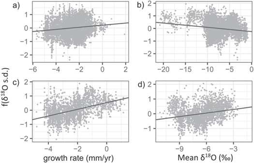
Figure 2. Partial residual plots from multiple linear regression analysis, showing the relationship between the standard deviation of speleothem δ18O (δ18Ospel s.d.) and two predictor variables: growth rate and mean δ18O (as an indicator of mean climate). Speleothem data is separated into northern hemisphere (top panel) and southern hemisphere (bottom panel) sites. All relationships are significant with P values < 0.001.
Download figure:
Standard image High-resolution image3.2. Regional δ18Ospel variability evolution
Three regions have sufficient data to reconstruct composites of IADVspel: the Indian Monsoon (ISM), East Asian Monsoon (EAM) and South American Monsoon (SAM) (figure 1). The Central American and Indonesian-Australian monsoon regions are excluded because they contain too few records of a sufficient length. The regional evolution of corrected and uncorrected IADVspel is very similar (figure 3), confirming that changes in growth rate (or n-samples) and mean δ18Ospel are not the main cause of the reconstructed changes in δ18Ospel variability during the Holocene. Any uncertainty arising from combining records of different lengths is small, based on bootstrap resampling (figure S2). Regional composites show a significant amount of centennial-scale variability, nevertheless broad trends can be seen, with differing IADVspel evolution between the three regions.
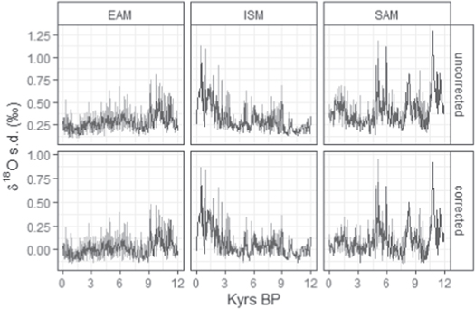
Figure 3. Evolution of regional speleothem δ18O standard deviation (δ18Ospel s.d.) values through the Holocene. Trends are shown with uncorrected values and values with a correction applied, using the relationships constrained in the multiple linear regression model. Regional monsoons are EAM = East Asian Monsoon, ISM = Indian Summer Monsoon, SAM = South American Monsoon. δ18Ospel s.d. values are extracted using a 100-year windows with 50% overlap. Regional composites are expressed as a running median with confidence intervals represented by 5% and 95% quantiles.
Download figure:
Standard image High-resolution imageTable 2. Linear regression relationships of regional δ18Ospel s.d. versus time and simulated precipitation s.d. trends versus time (mm/month yr−1) from the mid-Holocene (6 000 years BP) to 0 years BP. Negative relationships represent lower variability (s.d.) at the mid-Holocene than at present. Significant relationships (P <0.0001) are shown in bold. EAM = East Asian monsoon, ISM = Indian Summer monsoon, SAM = South American monsoon.
| spel 6–0ka | IPSLCM5A-LR | IPSL-Sr | AWI-ESM2 | MPI-ESM1.2 | |
|---|---|---|---|---|---|
| EAM | 0.015 | −1.17E-05 | −1.01E-05 | 9.96E-07 | −2.34E-07 |
| ISM | −0.061 | −1.22E-05 | −2.51E-05 | −1.96E-05 | −1.26E-05 |
| SAM | 0.020 | 1.49E-07 | −4.85E-06 | −6.40E-06 | −1.89E-06 |
The EAM IADVspel record is decomposed into four segments (figure 4(a), table S2): The early Holocene interval (12 to 8.9 ka) has significantly higher IADVspel than any subsequent period. The following interval between 8.9 and 7.1 ka has significantly lower IADVspel than the early Holocene interval. The mid-Holocene interval (7.1 to 2 ka) shows a significant increase in IADVspel. The last 2 000 years has significantly lower IADVspel than any preceding interval. The ISM IADVspel record is decomposed into three segments (figure 4(b), table S2): the early Holocene (12 to 9 ka) has significantly lower IADVspel values than the other two periods. The mid-Holocene period (9 to 1.7 ka) has significantly lower IADVspel than the period after 1.7 ka. Breakpoint analysis of the slopes (figure S3, table S3) show stable IADVspel values, except between 2.05 and 0 ka when they show a significant increase over time. The SAM IADVspel record is decomposed into four segments (figure 4(c), table 3). The highest values of IADVspel occur in the mid-Holocene (6 to 4.2 ka) and the early Holocene (12 to 10.15 ka). The interval between these two peaks is characterised by IADVspel values that are statistically indistinguishable from the past 4 000 years. Although the recent interval shows stable variability (figure S3, table S3), the earlier part of the SAM record shows increases in variability with rapid transitions to lower variability at 10.15, 7.9 and 4.75 ka.

Figure 4. Breakpoint models (IADVspel ∼ 1) of regional IADVspel evolution. Breakpoints are shown with their 2.5 and 97.5% confidence intervals. Step changes in IADVspel are shown. Regional monsoons are EAM = East Asian Monsoon, ISM = Indian Summer Monsoon, SAM = South American Monsoon.
Download figure:
Standard image High-resolution imageTable 3. P-values for pairwise t-test, with the null hypothesis that the mean difference between two segments is zero. Segments are separated for each regional monsoon by breakpoint analysis, where the timings of abrupt changes (IADVspel ∼ 1) were determined. Regional monsoons are: EAM, East Asian monsoon, ISM, Indian summer monsoon, SAM, South American monsoon. Bold values indicate P-values <= 0.001, where the null hypothesis can be rejected.
| Segments (years BP) | Mean s.d. | P-values | |||
|---|---|---|---|---|---|
| EAM | 0–2000 | 2000–5950 | 5950–8800 | 8800–12000 | |
| 0–2000 | −0.049 | / | |||
| 2000–7100 | 0.015 | 7.88E-07 | / | ||
| 7100–8900 | −0.045 | 7.78E-01 | 6.13E-06 | / | |
| 8900–12000 | 0.069 | 5.20E-16 | 2.28E-06 | 3.44E-14 | / |
| ISM | 0–2150 | 2150–9000 | 9000–12000 | ||
| 0–1700 | 0.198 | / | |||
| 1700–9000 | 0.022 | 1.10E-17 | / | ||
| 9000–12000 | −0.024 | 2.21E-20 | 4.62E-03 | / | |
| SAM | 0–4200 | 4200–7900 | 7900–10150 | 10150–12000 | |
| 0–4200 | 0.051 | / | |||
| 4200–6000 | 0.1942 | 1.40E-06 | / | ||
| 6000–10150 | 0.046 | 8.20E-01 | 8.83E-07 | / | |
| 10150–12000 | 0.234 | 1.04E-09 | 1.49E-01 | 8.65E-11 | / |
3.3. Comparison with simulated monsoon variability
There is no overall change in IADVspel over the last 6 000 years in the EAM (table 2), reproduced by the AWI and MPI simulations (table 2). The IPSL simulations show a small but significant increase in IADVprecip through time. The significant increase in IADVspel from 6 onwards in the ISM is reproduced by all four simulations (figure 5, table 2). There is no significant change in IADVprecip through time in the SAM in any simulation (figure 5, table 2), whereas IADVspel increases significantly through time. However, this is driven by the peak at 4.2 to 6 ka; a linear regression from 5 ka onwards shows no significant change.
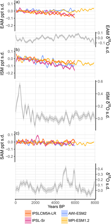
Figure 5. Evolution of regional speleothem δ18O standard deviation (δ18Ospel s.d.) values through the Holocene, compared to regional precipitation standard deviation simulated by four transient Earth System Models. Regional monsoons are: (a) EAM, East Asian Monsoon, (b) ISM, Indian Summer Monsoon, (c) SAM, South American Monsoon. Precipitation and δ18Ospel s.d. values are extracted for 100-year windows with 50% overlap. Precipitation s.d. values are calculated as anomalies to the last 1 000 years. Trends are fitted with a smoothed loess fit (500-year window).
Download figure:
Standard image High-resolution imageThere are significant changes in simulated IADVprecip between the segments identified from the speleothems (table 4). In the ISM, all four simulations show significantly higher IADVprecip in the 1.7 to 0 ka period than the preceding period (table 4), consistent with the IADVspel record. All simulations show a significant increase in IADVprecip values from 1.7 ka onwards, but no significant trend prior to this (Table S4). This is consistent with the marked increase in IADVspel during the most recent 1 700 years. In the EAM, the AWI and MPI simulations show no significant difference in either slope or magnitude between the two intervals. (tables 4, S4), whilst the IPSL simulations show higher IADVprecip values for the most recent 2 000 years compared to the prior period. There is no significant difference between the intervals before and after 4.2 ka in SAM IADVprecip and neither interval shows significant changes in IADV through time (tables 4, S4). This is not consistent with the speleothem record, which shows higher variability before 4.2 ka than after.
Table 4. Mean regional precipitation s.d. values for Holocene segments, identified in the breakpoint analysis of the speleothem trends. Bold values show segments (within an individual region and model) that are significantly different from the other (P <0.0001), determined using pairwise t-test. Regional monsoons are: EAM, East Asian monsoon, ISM, Indian summer monsoon and SAM, South American monsoon.
| Region | Segments | IPSLCM5A-LR | IPSL-Sr | AWI-ESM2 | MPI-ESM1.2 |
|---|---|---|---|---|---|
| EAM | 0–2000 | 0.310 | 0.357 | 0.274 | 0.271 |
| 2000–6000 | 0.274 | 0.327 | 0.271 | 0.277 | |
| ISM | 0–1700 | 0.355 | 0.465 | 0.479 | 0.413 |
| 1700–6000 | 0.313 | 0.389 | 0.418 | 0.370 | |
| SAM | 0–4200 | 0.442 | 0.448 | 0.277 | 0.305 |
| 4200–6000 | 0.441 | 0.434 | 0.255 | 0.293 |
3.4. Relationship between monsoon variability and long-term evolution
Speleothems and simulations show no consistent relationship between IADV and long-term changes in monsoon precipitation. There is declining summer monsoon strength and regional precipitation from the mid-Holocene onwards in the EAM and ISM, with a slower decline from ∼ 2 ka, following NH summer insolation (figure 6). However, IADV evolution differs between these two regions. In the EAM, the decreasing monsoon strength is mirrored by a decrease in IADVspel (figure 7(a), table 5). This relationship is reproduced by the AWI and MPI simulations, although only MPI shows a significant relationship between mean precipitation and IADV. In contrast, the declining summer monsoon strength from the mid-Holocene onwards is accompanied by increasing IADV amplitude in the ISM. This relationship is reproduced by all four simulations. SAM observations and simulations show a strengthening monsoon from the mid-Holocene onwards (figure 6(e)), mirroring SH summer insolation (figure 6(d)). There is no significant relationship between the long-term changes and IADVspel in the SAM. The lack of a relationship is reproduced by three of the four simulations (table 5).

Figure 6. Comparison of summer insolation with long-term evolution of monsoon mean state through the Holocene. Regional speleothem δ18O trends are represented by smoothed (500-year half-window loess fit) z-scores with respect to a base period of 3 000 to 5 000 years and 100 year mean z-score values (dark red line). Simulated monsoon evolution is represented by region-averaged summer precipitation (May to September for Northern Hemisphere monsoons, November to March for Southern hemisphere monsoons), as anomalies to 0–1 000 years BP. Insolation values are calculated as summer means (May to September for Northern hemisphere monsoons, November to March for Southern hemisphere monsoons). Regional monsoons are b) East Asian monsoon (EAM), c) Indian summer monsoon (ISM) and e) Southern American monsoon (SAM). Note that the y-axes for δ18Ospel z-scores have been reversed to match the negative relationship of δ18Ospel with monsoon strength and summer insolation.
Download figure:
Standard image High-resolution image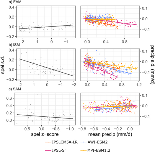
Figure 7. Relationships between the long-term evolution of the regional monsoons (x-axes) and their variability (y-axes). We use regional speleothem δ18O z-score data and mean precipitation for 100 year sliding windows to represent long-term changes in monsoons for speleothem data and modelled precipitation respectively. Variability is represented by the standard deviation of δ18Ospel and precipitation for 100 year sliding windows. Regions are a) EAM, East Asian monsoon, b) ISM, Indian Summer monsoon and c) SAM, South American monsoon. For each region, we show the results from four climate model simulations. Note that the axes for δ18Ospel z-scores have been reversed to match the negative relationship between δ18Ospel and monsoon strength.
Download figure:
Standard image High-resolution image
Table 5. Linear regression relationships of s.d. values (δ18Ospel s.d., regional precipitation s.d.) versus long-term evolution (δ18Ospel z-score, mean 100-year regional precipitation). Significant relationships (P <0.0001) are shown in bold. Regions are EAM = East Asian monsoon, ISM = Indian Summer monsoon, SAM = South American monsoon. Note that more negative δ18O z-scores and higher regional precipitation values represent a stronger monsoon, therefore agreement between speleothem data and models will be opposite direction trends.
| Region | Spel | IPSLCM5A-LR | IPSL-Sr | AWI-ESM2 | MPI-ESM1.2 |
|---|---|---|---|---|---|
| EAM | −0.0245 | −0.102 | −0.055 | 0.016 | 0.027 |
| ISM | 0.0556 | −0.083 | −0.178 | −0.105 | −0.051 |
| SAM | 0.105 | 0.004 | 0.03 | 0.059 | 0.017 |
4. Discussion and conclusions
We have shown that variable growth rate, sampling frequency and mean climate have a minimal impact on δ18Ospel variability overall. Although cave monitoring studies have emphasised the influence of site-specific factors on δ18Ospel (Luo et al 2014, Wu et al 2014, Pu et al 2016), these factors are unimportant when records from different speleothems and cave sites are combined. This is expected because, unlike climate signals, site-specific factors that might affect growth rate are unlikely to be consistent across sites. It might be useful to take account of the residence time of water in the epikarst directly in reconstructing δ18Ospel variability, but this is hard to quantify under the changing climate conditions of the geological past and may be unnecessary given that climate conditions that influence residence time may be indirectly incorporated via mean δ18Ospel. Despite the simplicity of our MLR model, the relationships between IADVspel and the predictor variables are physically plausible and corrected IADVspel evolution is similar between speleothems and sites.
Regional IADVspel changes cannot be compared with the Galapagos Islands and Ecuador lake records which are interpreted as ENSO frequency rather than IADV amplitude. However, the hydrogen isotope record from El Junco (Zhang et al 2014), which is interpreted as a record of El Niño amplitude, shows large multi-centennial scale fluctuations in the early to mid-Holocene like those in SAM IADVspel. Indeed, numerous records show fluctuations of a similar nature, including tropical Pacific reconstructions (Carré et al, 2021) and the Lake Pallcacocha records (Moy et al 2002). The low amplitude variability recorded at El Junco during the mid-Holocene and the abrupt shift to present-day variability at ∼3.5 ka is also similar to the ISM IADVspel record. ISM and SAM IADVspel shows similarities with regional reconstructions of IADV amplitude from the tropical Pacific (Carré et al 2021). The western Pacific shows lower IADV through the early to mid-Holocene, then an abrupt shift to modern levels at ∼2 ka, similar to ISM IADVspel, whilst central Pacific records show a peak in IADV at ∼6 ka, similar to the peak in SAM IADVspel at this time. Thus, the speleothem composites provide a coherent picture of regional changes in IADV that are broadly consistent with other Holocene IADV reconstructions.
Some features of the IADVspel records are reproduced by the models. Simulated IADV evolution reproduces the higher IADV of the last 1 700 years compared to the mid-Holocene seen in ISM IADVspel and the lack of an overall long-term Holocene changes in IADVspel in SAM. The AWI and MPI simulations show differing trends between the ISM and EAM, as seen in the IADVspel records. There are, however, differences between speleothem and simulated IADV changes. The IPSL simulations show increasing IADV from the mid-Holocene to present for the EAM, whereas IADVspel decreases. However, these simulations show smaller changes in IADV in the EAM than the ISM and thus there is a difference in ISM and EAM simulated IADV even though this differentiation is less marked than the opposite changes seen in regional IADVspel. The models do not show the large multi-centennial scale fluctuations seen in SAM IADVspel. Comparisons of simulated and reconstructed SST IADV in the tropical Pacific also show that these models exhibit less multi-centennial variability than coral and bivalve records (Carré et al 2021). These discrepancies between simulated and reconstructed IADV, and indeed between different models, strongly suggests that the controls on monsoon precipitation are only indirectly tied to changes in external forcing.
The long-term evolution of regional precipitation follows summer insolation (figure 6), but changes in regional monsoon IADV do not show a direct relationship with insolation. Long-term precipitation changes in the EAM and ISM are similar, but IADV evolution differs and even the abrupt change in IADV at ∼ 2 ka has a different sign in the two regions. Analyses of marine records from the Pacific (Carré et al 2021) suggests that there is a link between orbital forcing and ENSO variability, but ENSO is not the only cause of changes in rainfall IADV in monsoon regions.
Differences in the relationship between simulated long-term evolution and precipitation IADV between the Indian and west African monsoons have been explained as reflecting the important role of ENSO over India and Atlantic modes over west Africa for precipitation variability (Braconnot et al 2019a). Differences in regional IADVspel evolution presumably also reflects the importance of different modes for IADV in each region. In the present-day, IADV over the EAM is influenced by ENSO signals that may also be modulated by the Pacific Decadal Oscillation (Feng et al 2014, Zhang et al 2018), whilst the ISM may also be influenced by changes in the Indian ocean (Ashok et al 2004, Krishnaswamy et al 2015). SAM IADV is influenced by changes in the tropical Atlantic and Indian Ocean, as well as ENSO (Grimm and Zilli 2009, Yoon and Zeng 2010, Jimenez et al 2021). Furthermore, each monsoon region has a distinct relationship with ENSO, with the nature and strength of the precipitation responses depending strongly on the location of SST anomalies in the tropical Pacific (Kumar et al 2006, Tedeschi et al 2015, Zhang et al 2016). All these regions show a changing relationship with ENSO in recent decades (Samanta et al 2020, Seetha et al 2019, Zhang et al 2018, Wang et al 2020) and this was likely the case during the Holocene. In the ISM region, for example, a weakening of the monsoon precipitation-ENSO relationship in recent decades has been attributed to a warming Eurasian continent (Kumar et al 1999), changes in tropical Atlantic SSTs (Kucharski et al 2007) and influence from the IOD (Ashok et al 2001). Analysis of ISM IADV evolution in the IPSL simulations (Crétat et al 2020) emphasised the interaction between ENSO, IOD and ISM precipitation variability. In the East Asian monsoon, the observed changing relationship between monsoon precipitation and ENSO over the last millennium is attributed to interaction with the PDO (Zhang et al 2018). Reconstructions and model simulations show changing PDO-like variability through the Holocene, including a positive phase during the early Holocene (Chen et al 2021). It is therefore likely that the relationship between EAM precipitation variability and Pacific SSTs was significantly different during this period. Since regional monsoon precipitation variability is influenced by numerous modes that can interact with one another, it is likely that the lack of a direct and linear relationship between monsoon IADV and insolation through the Holocene reflects the complexity of these influences on regional precipitation and the potential for changes in the importance of different climate modes through time. More emphasis should therefore be placed on modes of variability other than ENSO to improve our understanding of the evolution of monsoon climate during the Holocene, using high resolution terrestrial records and model simulations.
Acknowledgments
SP and SPH acknowledge support from the ERC-funded project GC2.0 (Global Change 2.0: Unlocking the past for a clearer future, grant number 694481). SPH and PB acknowledge support from JPI-Belmont Forum project Palaeo-climate Constraints on Monsoon Evolution and Dynamics (PACMEDY). We acknowledge the modelling groups of Institut Pierre Simon Laplace, Alfred Wegener Institute and Max Planck Institute for producing and sharing the climate simulations. We thank Laia Comas-Bru for helpful discussion on the speleothem analysis.
Data availability statement
The data that support the findings of this study are openly available at the following URL/DOI: https://doi.org/10.5281/zenodo.5084426 (Parker 2021).
Data and code availability
The code used to generate the results and figures in this study are available at (doi.org/10.5281/zenodo.5084426; Parker 2021). SISAL version 2 is available at http://doi.org/10.17864/1947.256. We use R for analyses (R Core Team 2019). The main packages used are tidyverse (Wickham et al 2021), ggplot2 (Wickham 2016), RMySQL (Ooms et al 2020) and ncdf4 (Pierce 2019).