

Abstract
San Clemente Island (SCI), located in the Southern California Bight, is owned and operated by the U.S. Navy and is home to endemic species, including federally threatened or endangered plants and birds. The SCI ecosystem is influenced by the presence of warm season low-level clouds that shade, cool and, especially when in the form of fog, moisten the environment. We created a new cloud and fog satellite-derived albedo product for SCI at a higher resolution than previous datasets. The record spans 23 summers (1996–2018, May - Sep). The spatial resolution is ∼1 km and the temporal resolution is half hourly (nominally 0600 to 1800 PST). Using Geostationary Operational Environmental Satellite (GOES)-WEST visible band measurements, it was discovered that small (typically on the order of less than 5 km) geographical misalignment of the satellite images was common. The biological ramifications of such a shift could be significant. Thus, to provide a useful 1 km product for a narrow island such as SCI it was necessary to correct misalignments. Misalignment of albedo was easily apparent in clear sky images at the interface of land and water. This concept was used in the automated correction. The northwest coast of SCI is the cloudiest/foggiest area. June, on average, is the cloudiest month on SCI. The intra-day variability reaches ∼20% cloud albedo while interannual and monthly variability are ∼10%. To demonstrate the records' utility in understanding ecological phenomena and patterns, we used the dataset to model plant distributions. We found monthly mean cloud albedo values, a proxy for cloud frequency and persistence, were among the most important environmental variables in understanding plant distributions. The vegetation models indicate locations with appropriate conditions, including clouds and fog during critical periods of the year, for particular vegetation types and thus, can inform restoration and management activities.
Export citation and abstract BibTeX RIS
1. Introduction
Low-level stratiform (blanket-like) clouds and fog, which is a cloud with base at surface level, are persistent warm season features of continental west coasts, including in the Southern California Bight. These coastal low clouds and fog (CLCF) or, colloquially, marine layer clouds or May Gray and June Gloom, provide critical summertime shading, cooling, and moisture to the coastal environment during the otherwise dry summers indicative of the region's Mediterranean climate. A key factor to formation and maintenance of these low-level cloud sheets is a persistent and low-level temperature inversion which acts as a stable lid capping the marine boundary layer and inhibits mixing. The temperature inversion results in part from adiabatic warming of descending air from the global scale Hadley circulation. Due to upwelling and cold advection, coastal California waters are relatively cool and when moist marine air reaches saturation, a low-level cloud layer forms and the inversion defines the cloud-top. Efficient longwave cooling at cloud top strengthens the temperature inversion and drives mixing within the marine boundary layer, which in turn promotes continued cloud formation (Lilly, 1968, Wood, 2012). Other locations across the globe with similar air and sea ingredients (i.e., along eastern boundary currents of the subtropics) also experience seasonally persistent marine stratiform clouds and CLCF at their costal interfaces (Klein and Hartmann, 1993).
Through their effects on ecosystem water balance, CLCF are important drivers of coastal ecosystem processes including fluctuations in the size and structure of populations, interspecific competition, vegetation growth and senescence, phenology, nutrient cycling, and wildfires (Manzoni et al 2012, Carbone et al 2013, Emery et al 2018, Lawson et al 2018). CLCF are particularly important in Mediterranean systems because they mitigate ecological water deficits during the regular dry season and long-term droughts. Because they are difficult to quantify, the effects of fog and coastal low clouds have been poorly studied, although information is accumulating. The influence of these low clouds on coastal pine ecosystems of Santa Rosa and Santa Cruz Islands has been studied in some detail (Williams et al 2008, Carbone et al 2013, Baguskas et al 2014). While most work has been done in systems with higher levels of CLCF, even where fog water is insufficient to change soil moisture, ecosystem effects can be significant (Breshears et al 2008, Vasey et al 2012). In shrublands and native perennial grasslands, both of which are widespread on San Clemente Island (SCI), CLCF influences species distributions and community composition and diversity (Axelrod 1978, Corbin et al 2005, Vasey et al 2012).
Fog water input has been shown to be an important water source influencing plant demographics on Santa Catalina Island (Evola and Sandquist 2010). SCI, about 40 km south of Catalina, is currently recovering from long term feral ungulate grazing that resulted in extensive type conversion from shrublands to non-native grasslands (Raven 1963, SERG 2015). With the removal of non-native grazers in the early 1990s, woody habitats are increasing as evidenced by recent vegetation mapping (Uyeda et al 2020 ). CLCF likely plays an important role in the process of shrub recolonization by promoting shrub establishment through increased seedling summer survival rates in non-native grasslands. As those seedlings grow, their woody structure functions to precipitate fog water out of the air. Thus, these individual shrubs create mesic microsites promoting further shrub seedling establishment and recruitment (Woolsey et al 2018). Development of this spatially refined satellite-derived CLCF record is anticipated to improve understanding of the role of CLCF in this process on SCI and should help promote the design of more cost-effective conservation strategies. While previous work of this type has not focused in detail on SCI, CLCF likely has a significant impact and management stands to benefit from the incorporation of CLCF data into biological monitoring and management programs.
Previous research has described California low cloud variability and its physical drivers over a wide range of scales from broad-scale climate (Johnstone and Dawson 2010, Schwartz et al 2014) to seasonal (Clemesha et al 2016) to local weather scales (Clemesha et al 2017) and during heat wave events (Clemesha et al 2018). Satellite records of low clouds and fog have been previously derived from Geostationary Operational Environmental Satellite (GOES)-West (Clemesha et al 2016, Torregrosa et al 2016). While the ∼4 km spatial resolution of these previous records was sufficient for studies of the whole California coast, for a narrow island like SCI, any nuanced study of the cloud cover and its effect on ecosystems requires a product with higher spatial resolution.
In the wake of feral ungulate removal, SCI resource managers are pursuing efforts to restore the native vegetation of these biodiverse ecosystems. Habitat suitability models are a key tool to inform current vegetation restoration efforts. Moisture from fog and microclimate conditions associated with cloud cover are important environmental conditions that influence the distribution of coastal plant species in California (Fischer et al 2009, Emery 2016) and in particular on SCI (Schoenherr et al 1999). We developed a new satellite-derived cloud and fog dataset and investigated its usefulness in explaining the distribution of the major vegetation groups on SCI by incorporating them into these habitat suitability models along with other important geophysical features to see if these layers add additional explanatory value.
2. Materials and methods
2.1. Creation of new 1 km satellite-derived cloud albedo record
We created a new cloud and fog albedo satellite-derived product for SCI at a higher resolution than previous datasets (Clemesha et al 2021). The record spans 23 summers (1996–2018, May–Sep). The spatial resolution is 1 km centered on SCI (spatial boundaries: 32.6 °N to 33.2°N and 118.8°W to 118.2°W) and the temporal resolution is half hourly (nominally 0600 PST to 1800 PST).
To create this new record for SCI, we used GOES − 9, 10, 11, and 15 Imager visible measurements which have a nominal 1-km field of view. For GOES-9, 10, and 11 the visible channel is centered on 0.65 μm (range 0.52 μm to 0.8 μm). For GOES-15 the visible channel is centered on 0.63 μm (range 0.52 μm to 0.71 μm). The original raw GOES variable format (GVAR) data used in all processing was obtained from University of Wisconsin for 1996–2008, and for 2009–2018 from the National Oceanic and Atmospheric Administration (NOAA), Comprehensive Large Array-Data Stewardship System (CLASS) (www.class.noaa.gov). As described by Iacobellis and Cayan (2013), the raw GVAR data was converted to albedo using NOAA pre- and post-launch calibration procedures (www.star.nesdis.noaa.gov/smcd/spb/fwu/homepage/GOES_Imager.php). As shown by Wu and Sun (2005), the post-launch calibrations significantly reduce the variability introduced by changing GOES visible sensors.
Albedo is a measure of reflectivity, defined as the percent of reflected radiation to incident radiation commonly integrated across either the whole solar spectrum or the visible portion. The range of visible albedos for natural surfaces ranges from as low as ∼4% for calm ocean waters and overhead sun to more than ∼80% for thick clouds (American Meteorological Society 2020). In this study, as in Iacobellis and Cayan (2013), cloud albedo is measured using the visible channel of GOES and is used as a proxy for cloudiness. Thus, here, cloud albedo refers to the reflectivity of radiation integrated over the visible band as measured by GOES. All clouds and fog (except for thin high-altitude cirrus clouds) typically have high visible reflectance relative to a clear sky background. As cloud cover and/or cloud thickness increase, visible band reflectivity increases and the amount of visible radiation reaching the surface decreases. Cloud albedo can conversely be thought of as quantifying the amount of visible radiation that is blocked from reaching the surface. Consequentially cloud albedo is directly linked to any surface processes dependent on incoming visible radiation such as net radiation, temperature and the convective heat fluxes.
Cloud (or fog) albedo is determined by subtracting clear sky albedo (the reflectivity of cloud-free land and ocean surfaces) from the total albedo measured by GOES. During the determination of clear sky albedo scenes, it was discovered that small (typically on the order of less than 5 km) geographical misalignment of the satellite images was common. Although not an issue in most applications in which GOES satellite visible measurements have been used, the biological ramifications of such a shift could be significant. Thus, to provide a quality 1 km product for a narrow island such as SCI, it was necessary to correct any misalignment (see appendix A for details).
Once the alignment correction was complete, an accurate clear-sky albedo value was calculated as the 1st percentile of albedo values over 23 years (1996–2018), for each pixel, month, and time of day. Clear-sky albedo values were calculated for different times of day because cloud albedo increases with increasing solar zenith angle, i.e. towards early morning and late afternoon.
As in Iacobellis and Cayan (2013) and Rastogi et al (2016), we use higher cloud albedo values as a proxy for low-level cloudiness and the analysis is restricted to the months of May to September when the low-level clouds are the dominant cloud type. Time-averaged cloud albedo results, as presented in 3. Results and Discussion, represent the frequency and persistence of low-level clouds. Cloudiness, as referred to in this study, is not meant to be an exact measure of the horizontal extent of clouds covering a specific area. Rather, it is an estimate of the amount of visible band radiation that is prevented from reaching the surface due to the presence of CLCF. The resulting geographically aligned 1 km cloud albedo record was validated using hourly cloud cover observations at the SCI airfield. Retrieval performance compares well with other satellite derived products (appendix A), and this validation supports our use of cloud albedo as a proxy for low-level cloudiness.
2.2. Vegetation distributions models
Environmental niche modeling for vegetation is used as a demonstration case for the cloud albedo record. We used a machine-learning approach, which takes the known locations of different vegetation occurrences and identifies what environmental characteristics, including the cloud albedo conditions during different months, are associated most strongly with them. We used the open source software Maxent (Phillips et al 2017) to model vegetation distributions. A high-resolution vegetation map for SCI was obtained from the US Navy (McDermott and Nieto 2012, Uyeda et al 2020). Plant distributions were mapped for individuals and different levels of vegetation classification, as defined by the U.S. National Vegetation Classification System, including Associations, Alliances, and Macrogroups (see www.usnvc.org). From those categories, we selected native groups, with the exception of grasslands, which encompassed native and exotic grasslands. We combined the vegetation polygons and from within each vegetation classification we extracted a random sample of points to be used as test and training points. We specified 3 meters as the minimum distance between each point and from polygon boundaries. Sample sizes ranged from 100 to 2,480 points and representation was proportional to the log-transformed area of that species or vegetation group across the island, which allowed less-common vegetation classifications, individually recorded species, and dominant vegetation units to each be modelled more realistically. A random sample of locations that represents the full breadth of suitable environmental conditions for occurrence is valuable to create better estimates of geographic distributions and to understand relationships with associated environmental variables (Phillips et al 2017).
We developed a set of environmental layers from a digital elevation model derived from LiDAR in 2016 (Chadwick et al 2016). Aspect was transformed (sin (h + 45°)) into a continuous variable that represents an index of north-eastness, a variable that is a proxy for rainfall in this environment. An orientation to the northeast is associated with cooler and wetter conditions. A topographic wetness index was derived that combined upslope water flow accumulation with slope gradient to differentiate pixels by their moisture-retention potential. We calculated an insolation raster to estimate direct and diffuse radiation received at the surface under clear-sky conditions using the solar radiation tools in ArcGIS Pro (Esri, Redlands, California). These two secondary land surface parameters inform environmental research at a landscape or regional scale (Wilson 2018). We mapped and aggregated soil associations (USDA-NRCS 2019) to create a simplified texture, permeability, and water-holding capacity index, which we converted to a 3-m raster dataset. We included the monthly measurements of cloud albedo for May through September (1996–2018); we clipped and re-sampled original data to produce 3-m resolution rasters for each month.
We checked for correlation between all environmental variables and ran initial models with 16 variables, which we then reduced to 10 variables, leaving out those that had low contribution as measured by permutation importance and variable importance. We kept each of the five months of time-averaged cloud albedo (higher values representing more low cloud presence) even though some months were highly correlated with each other, because of the high value of these layers in initial model testing. Under normal circumstances the albedo layers would have been reduced to a single layer given their high correlation, but because the consequences of conflating the effects of two different months would be less than the insight gained from investigating the influence of seasonal patterns, we kept all five layers in the models.
We then ran suitability models with 50 replicates and 25 percent random test points withheld in each model run, subsampling points for each replicate. Various feature classes are used by the modelling software to create response curves for each variable. These were constrained to linear, quadratic, and hinge (piece-wise linear) functions, omitting product features to create simpler models that are more easily interpreted. Model fit and performance were assessed using Maxent's test gain and Area Under Curve (AUC) statistics (Merow et al 2013, Phillips et al 2017). Outputs were mapped using the complementary log-log link function, which can be interpreted as probability of presence or suitability (Fithian et al 2015). This interpretation is built on the interpretation of Maxent as a point-process statistical model, which gives maximum entropy species distribution modelling another theoretical justification (Renner et al 2015), and also treats presence-only occurrences as points rather than grid cells (Phillips et al 2017).
2.3. Other weather and climate datasets
The variability of West Coast CLCF has been shown by others (Johnstone and Dawson, 2010, Schwartz et al, 2014) to be linked with the Pacific Decadal Oscillation (PDO- Mantua et al 1997). The PDO index is the first principal component of monthly sea surface temperature variability in the North Pacific and represents a coupled pattern of climate variability in the upper ocean and atmosphere of this region. We obtained the monthly PDO index from the University of Washington (http://jisao.washington.edu/pdo) to investigate this relationship with the new SCI CLCF record. To investigate the impact of CLCF on surface temperatures, we obtained SCI weather station data from csun.edu/scisland/Observations.html and for later dates from Mesowest (mesowest.utah.edu). To validate the satellite retrieval and explain spatial patterns in cloud albedo patterns, wind data from the airfield (KNUC) were obtained from Mesowest and cloud cover at the airfield was obtained from NOAA's NCDC (https://www.ncdc.noaa.gov/data-access/land-based-station-data).
3. Results and discussion
3.1. Climatology of low clouds and fog on San Clemente Island
The new 1 km cloud albedo record provides a wealth of new knowledge about the weather and climate of SCI during the warm season (May—September). In this section, we describe the temporal variability of SCI daytime coastal low clouds and fog from the 23-year climatology to intra-day time scales. The full 23-year climatology of daytime cloud albedo is shown in figure 1(A) with elevation contours overlain. The northwest coast of SCI is the cloudiest/foggiest area, with the coast just west and northwest of Eel point reaching over 24% time-averaged cloud albedo. Mean cloud albedo contours are oriented southeast-northwest (with a greater northward component than the orientation of the island itself). Figure 1(B) shows 18 years of wind observations (speed and direction) from KNUC on the NW tip of SCI. Consistent with climatological west-northwest winds and elevation of SCI, the southeast part of the island is the clearest. The low cloud deck is interrupted by the higher terrain and clearing occurs at these higher elevations and on the lee side of elevated terrain.

Figure 1. (A) Cloud albedo (%) time-averaged over the full May to September, 1996–2018 1 km record. Higher albedo (red) denotes cloudier/ foggier climate with more frequent and persistent CLCF. Elevation contours (gray) are in meters. Locations of interest including the highest peak (Mt Thirst) at ∼600 m are marked. (B) Wind observations (speed and direction) from the airfield (KNUC). Both panels are for May to September.
Download figure:
Standard image High-resolution imageThe year-to-year range in cloud albedo averaged over SCI and surrounding nearshore waters (domain shown in figure 1) is about 8% (figure 2(a)). Summers 2001 and 2002 were anomalously cloudy island-wide, while 1996 and 2014 were the clearest summers on record (figure 2(a)). As also seen along the West Coast of North America (Schwartz et al 2014), there is a negative relationship between interannual variability in May to September cloudiness and the leading mode of North Pacific SST variability, known as Pacific Decadal Oscillation (PDO) index (Mantua et al 1997, figure 2(b)). For example, summers in which the PDO is in the negative phase, wherein eastern Pacific SSTs are anomalously cool, are associated with more frequent and persistent low-level cloudiness along the West Coast. Schwartz et al (2014) found this relationship to hold across interannual and interdecadal scales and lag-lead correlations indicate the SST patterns drive this relationship. Across SCI, the year-to-year cloud fluctuations over the windward (NW) part of the island are more correlated to PDO than over the rest of the island (figure B1). A cross-correlation analysis (see appendix B) reveals that cloud variability at Eel point is consistently representative of northwest SCI and at certain months and times of day representative of a wider area. May to September mean time series of PDO and cloud albedo at Eel Point are shown in figure 2(b) (r = − 0.45).
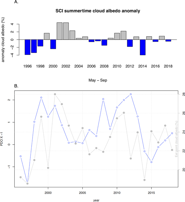
Figure 2. (A) May to September cloud albedo (proxy for cloudiness) anomaly (from long-term mean) by year averaged over the domain shown in figure 1 with gray bars denoting cloudier summers than usual and blue bars clearer than usual. (B) May to September cloud albedo at Eel point (gray) and −1 X PDO index (blue).
Download figure:
Standard image High-resolution imageJune, on average, is the cloudiest month on SCI with an average cloud albedo of 25% over the whole domain (figure 3). While spatial differences exist, island wide, May is the next cloudiest followed by July, August, and September all with between 15%–20% cloud albedo. Comparing July and May, northwest SCI is cloudier in July, while central and south SCI are clearer in July. August also has more clearing in the south than September does. These spatial-temporal differences can be explained by the seasonal cycle in the height of the low-level atmospheric temperature inversion base (which is the top of the low cloud layer) as reported by Iacobellis et al (2010) using radiosonde observations in San Diego. Due to enhanced subsidence in the North Pacific High and less frequent transient low pressure systems, the inversion base is typically lower in July and August than it is in May and September. A lower inversion base leads to a corresponding low cloud deck, which leads to more July clearing on the lee side (east and south sides) of SCI. The same is true for August (more lee side clearing) compared to September. The higher sensitivity of central and south SCI cloud cover to properties of the atmospheric vertical temperature profile also helps explain the lower correlation between PDO and interannual cloud variability in this part of the island (figure B1).
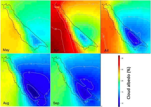
Figure 3. Monthly mean cloud albedo (proxy for cloudiness) for the full record 1996–2018.
Download figure:
Standard image High-resolution imageThe diurnal cycle is the time scale of greatest CLCF variability (figure 4). The intra-day range reaches ∼20% time-averaged cloud albedo while interannual and monthly scales exhibit a range of 10% time-averaged cloud albedo or less. In the northwest, 0600 PST cloud albedo is on average up to 37% and reduced down to 17% at 1200 PST. The greatest daytime clearing occurs in June. Over the island and nearshore waters, domain cloud albedo goes from over 40% in the early morning to less than 20% at midday. While a typical cloudy morning usually clears out (how quickly and how often depends on location), there are often instances of no daytime clearing. These fully overcast days are associated with much lower daytime temperatures, especially when compared against cloud-free days. For example, at the Nursery weather station (figure 4(b)) cloud-free days start out in the early morning (before 5 am) about 2°F warmer than fully overcast days, yet the difference increases to over 8°F from 900 to 1500 PST.
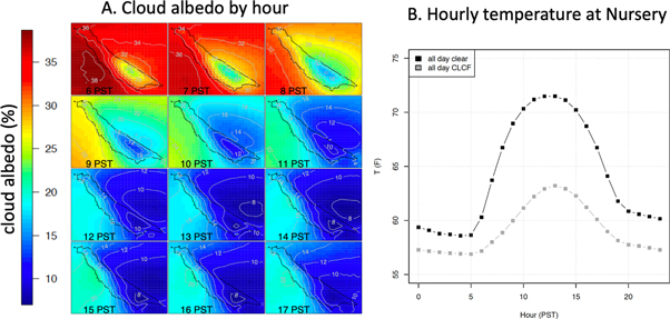
Figure 4. (A) Mean cloud albedo (proxy for cloudiness) by hour for the full record (May—Sep, 1996–2018). (B) Time series of mean hourly temperature at the Nursery weather station for days with CLCF present all day (cloud albedo > 20% for more than 20 daytime observations) and clear days (cloud albedo < 15% for more than 20 daytime observations).
Download figure:
Standard image High-resolution image3.2. Influence of coastal low clouds and fog on plant distributions
The plant distribution outputs were from 14 vegetation suitability models that used ten environmental variables each (figure 5). We kept the environmental variables the same for all models to be able to discern how these factors influenced, or did not influence, different vegetation alliance distributions. Most models produced excellent results with the test AUC greater than 0.9 (table 1). The high AUC values, combined with high test gain, indicate that the models built with training data accurately predict the occurrence of data withheld to test the model. Lower performing models were for the Californian Annual and Perennial Grassland Macrogroup, which encompasses a wide range of mostly non-native species, and Opuntia littoralis Shrubland Association.
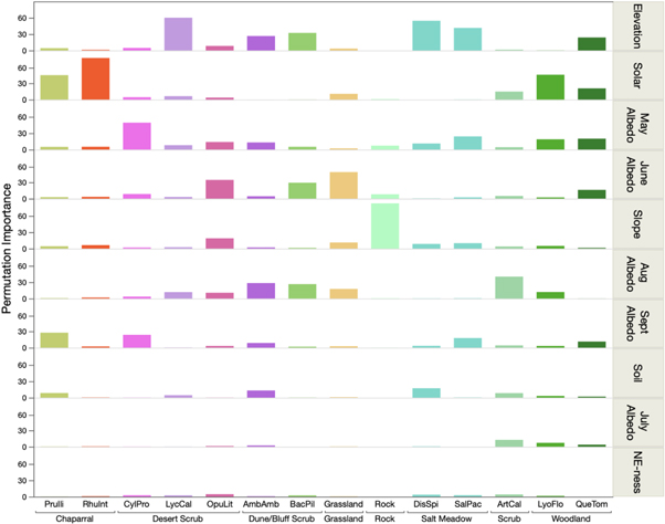
Figure 5. Permutation importance of each environmental factor on distribution models for fourteen vegetation classifications, sorted by group membership. Environmental variables are ranked from top to bottom by mean importance value across all models.
Download figure:
Standard image High-resolution imageTable 1. Vegetation groups modeled, with number of training points, test AUC, and test gain.
| Vegetation group | Number of training points | Test AUC | Test gain |
|---|---|---|---|
| Quercus tomentella (Species) | 342 | 0.99 | 9.6 |
| Lyonothamnus floribundus (Species) | 675 | 0.95 | 3.1 |
| Prunus ilicifolia (Species) | 643 | 0.94 | 2.6 |
| Ambrosia chamissonis-Abronia maritima Herbaceous Alliance | 1149 | 0.94 | 4.4 |
| Western North American Cliff, Scree and Rock Vegetation Macrogroup | 165 | 0.93 | >10 |
| Salicornia pacifica Herbaceous Alliance | 270 | 0.91 | >10 |
| Distichlis spicata Herbaceous Alliance | 75 | 0.90 | >10 |
| Cylindropuntia prolifera Shrubland Association | 1273 | 0.90 | 2.2 |
| Baccharis pilularis Scrub Alliance | 1223 | 0.90 | 2.0 |
| Rhus integrifolia (Species) | 1020 | 0.89 | 1.8 |
| Artemisia californica Shrubland Alliance | 1614 | 0.86 | 1.4 |
| Lycium californicum Desert Scrub Alliance | 1657 | 0.80 | 1.1 |
| Opuntia littoralis Shrubland Association | 1802 | 0.70 | 0.3 |
| Californian Annual and Perennial Grassland Macrogroup | 1860 | 0.68 | 0.3 |
The rank order of environmental variables by their permutation importance across all fourteen models was: elevation, insolation, May cloud albedo, June cloud albedo, slope, August cloud albedo, September cloud albedo, soils, July cloud albedo, and northeastness (see figure 5). Insolation is a measure of potential insolation under clear skies, which would be modified by low clouds and fog during the year. May and June albedos are likely important because they allow for retention of moisture and delay of drought stress during the latter portion of the growing season associated with winter rains.
Cloud albedo was particularly important in models describing distribution of the larger plants sensitive to drought stress (e,g, Prunus ilicifolia, Rhus integrifolia, Lyonothamnus floribundus), which are associated with lower elevations and higher cloud cover within canyons or on the northeast slope, compared with the more drought tolerant oak Quercus tomentella, found at higher elevations with less cloud cover. The cactus Cylindropuntia prolifera is very drought tolerant and associated with higher elevations with the lowest annual cloud cover, with its distribution being nearly perfectly defined by the minimum May, August, and September albedo. Lycium californicum at lower elevations was highly associated with higher presence of fog in all months. It is associated throughout its range with coastal succulent scrub that is supplemented by summer fog drip (Mooney 1988). Although this distribution is highly correlated with elevation, high June and July albedo is an even better standalone predictor than elevation for its distribution. Coastal sage scrub, which comprises summer deciduous plants such as Artemisia californica, was associated with low July and August albedo. This is consistent with its summer deciduous drought avoidance strategy, even though it is capable of opportunistically benefitting from late summer fog (Emery and Lesage 2015).
The vegetation models demonstrate an important use for the climatological description of cloud and fog cover. The development of high-resolution and accurate models of the environmental conditions associated with different vegetation types on SCI can also guide restoration and management actions. The models illustrate locations that have appropriate conditions, including clouds and fog during critical periods of the year, for particular vegetation types that are not currently found in those locations. Targeting such locations for reintroduction and restoration activities should have a high degree of success because the environmental conditions associated with occurrence elsewhere on the island are present. The cloud and fog distributions improve these distribution models considerably over alternatives lacking these data and thus demonstrate their usefulness to land management.
4. Conclusions
Coastal Low Clouds and Fog (CLCF) are an important driver of species and community dynamics and can have strong influences on ecosystem processes such as the hydrological cycle and fire. The 1 km cloud albedo record for the spring and summer months developed here opens the door for factoring the influence of CLCF on ecological studies or management actions on San Clemente Island (SCI). The application presented here demonstrating the contribution of spatial and seasonal patterns of CLCF to plant distributions is just one potential use of this data.
CLCF impacts a number of biologically relevant environmental variables including: daytime maximum temperature, nighttime minimum temperature, diurnal temperature range, surface insolation received, proportion of diffuse light received, evapotranspiration, direct water inputs and humidity (Lawson et al 2018). Depending on the anticipated mechanism for CLCF influence on target natural resources, other studies might use different summaries of the half-hourly albedo data to explain trends and phenomena. For example, live fuel moisture can be influenced by fog (Emery et al 2018); to investigate this, the albedo data could be averaged over the 24 h prior to the fuel moisture measurement and used in the analysis. Other variables could be constructed to identify e.g. the time of transition from overcast to clear skies and such a daily metric could be analyzed against daily weather variables to provide insight on processes driving diurnal clearing. Further development could involve expanding the cloud albedo record to the whole calendar year to allow for the detection of winter fog events. In conjunction with precipitation records, such a record would provide a fuller picture of the surface moisture budget.
An advantage of the new 1 km-grid dataset is that the whole cloud field over the island can be examined. Previously, long-term cloud cover observations were only available at the airfield or at coarser spatial resolution. Any specific locations of interest can be matched to the 1 km grid and extracted to create time series for analysis with other ecological or climate data observations. In addition, the fine spatial resolution allows identification of ecological patterns and spatial trends that could be obscured at coarser resolutions.
Acknowledgments
This work was supported by the US Army Corps of Engineers through Cooperative Agreement W9126G-17-2-0029 and by the US Navy through Cooperative Agreements W9126G-17-2-0040 and W9126G-12-2-0012 (TL). This study contributes to DOI's Southwest Climate Adaptation Science Center activities and NOAA's California and Nevada Applications Program award NA11OAR43101. We appreciate constructive conversations with John P Wilson. We thank Sam Iacobellis and Dan Cayan for providing expertise in remote sensing and climate science.
Data availability statement
The data that support the findings of this study are openly available at the following URL/DOI: https://weclima.ucsd.edu/data-products/.
Appendix A. Materials and methods
Appendix. A.1. Automated geographical alignment of satellite images
To correct small geographical misalignments of the satellite images we created an algorithm to correct misalignment so that we could provide a higher quality 1 km cloud albedo product for SCI. This correction needed to be automated since the record length covers over 75,000 images. It is easiest to automatically correct a visible satellite image that is of clear skies, but if enough precision is desired to observe differences in cloud and fog within SCI it is also critical to correct images that are cloudy at SCI. Figures A1 and A2 show examples of the original satellite albedo and the corrected versions for clear and cloudy SCI time periods, respectively and will be used to explain the alignment algorithm.
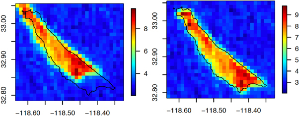
Figure A1. Example of albedo (%) on June 30, 1996 at 0900 PST (1000 PDT), a clear day at SCI. Map of the original satellite measurements (or 'satellite image') (left) and the corrected image (right). The misalignment of the albedo and coastline is clear in the left panel since dark ocean surfaces have a lower albedo than land surfaces. For a correct alignment the original image needed to be shifted 4 grid cells south and 4 grid cells east (each cell is 0.01°× is 0.0°1, ∼ 1 km × 1 km).
Download figure:
Standard image High-resolution image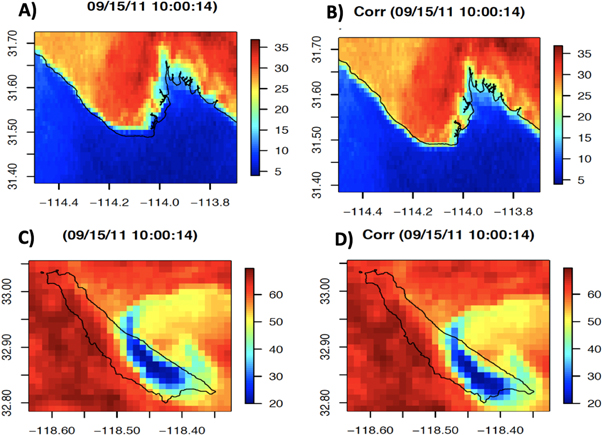
Figure A2. Example of albedo (%) on September 15, 2011 at 1000 PST, a cloudy time period at SCI. Maps of the original satellite measurements are shown on the left for (A) the interface between dark ocean waters and bright desert at the northern end of the Sea of Cortez in Baja California ('Delta') and (C) SCI. Maps of the corrected satellite measurements are shown on the right for (B) the Delta and (D) SCI. Misalignment is visible in the clear conditions of the Delta since dark water surfaces have a lower albedo than the bright desert surfaces. For a correct alignment the original image needed to be shifted 2 grid cells south and 1 grid cell east (each cell is 0.01° × is 0.01°, ∼1 km × 1 km). The alignment correction could not have occurred using albedo measurements near SCI because it was cloudy and thus the required contrast between land and ocean albedo is obscured by variation in cloud thickness. Note the different color scales of top and bottom panels as the island is cloudy (with albedo reaching over 60%).
Download figure:
Standard image High-resolution imageGeographical misalignment of albedo is easily apparent in clear sky images at the interface of land and water since land and water have such different natural reflectivity. This concept is used in the alignment correction, the steps of which are outlined below. (1) The GOES 1 km grid cells closest to the true coastline are identified. (2) For every original albedo image centered over SCI (+/− 5 cells in each direction) meridional differences in albedo (south-north) and zonal differences in albedo (west-east) are calculated. (3) The greatest positive and greatest negative meridional differences for every longitude and the greatest positive and greatest negative zonal differences for every latitude are found and marked as coastlines facing south, north, west and east, respectively. In a clear skies scene, the largest jump in albedo from one grid cell to the next should take place at coastlines and the sign of the change indicates either a transition to or away from lower albedo ocean/sea. (4) The overlap of these empirically determined coastline grid cells from step 3 with the known coastline grids of step 1 is calculated. (5) The empirically determined coastline grid cells are shifted up to 5 cells in every direction and the overlap of the shifted image coastline with the known coastline is calculated. (6) The best (highest value) overlap count between shifted and known coastline grid cells is selected as the best re-alignment.
The above procedure relies on clear skies conditions; thus, the procedure needs to be carried out elsewhere during cloudy or foggy conditions at SCI. The ideal candidate region for this is one impacted by a different cloud regime (so cloudy days at SCI are likely not cloudy days at this region) and with a large contrast between clear sky surface albedos. An ideal location was found at the northern end of the Sea of Cortez in Baja California (figure A3). Special modifications were then made to the above procedure and applied to this region. Safeguards to ensure that the alignment algorithm is not used inappropriately (that is when there is cloud present) are built into the procedure, and any alignments of poor quality (<25% potential coastline match value) are not made. The improvement in the number of overlapping coastline grid cells before and after the alignment correction is reduced during times of low sun angles because during these times an improved alignment is not found as often and thus a correction cannot always be made (figure A4).
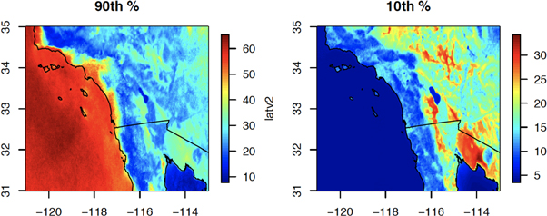
Figure A3. 90th percentile of albedo (left) and 10th percentile of albedo (right) for September 1000 PST (1996 to 2018). Note different color scales. These maps were used to help select a region to use in the alignment algorithm when SCI was cloudy. The coastline at the northern end of the Sea of Cortez in Baja California (called 'Delta'- see zoom in figure A2) was selected. Even during the top 10% highest albedo times in this region there is still over a 15% albedo contrast along the coast. The contrast is even greater on clear days (right).
Download figure:
Standard image High-resolution image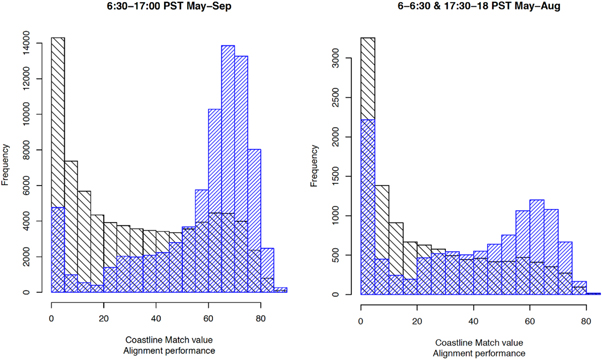
Figure A4. Histograms of the number of overlapping coastline grid cells (known/true coastline and 'coastline' as detected in each image) before alignment (black) and after alignment (blue). A higher coastline match value denotes better geographical alignment. Early morning and evening times 0600 PST, 1730 PST and 1800 PST for May-August are shown at right.
Download figure:
Standard image High-resolution imageNote during the shorter daylight hours experienced in September that cloud albedo could not be determined for the twilight hours of 0600 PST, 1730 PST and 1800 PST. Although cloud albedo is calculated for these time periods during May through August, higher uncertainty and missing data (set to NA for unexpected albedos of <0% or >100%) occur during these low sun angle time periods.
Appendix. A.2. Validation of satellite retrieval by comparison with airport observations
The cloud albedo record performs well when compared against airport observations of cloud cover at KNUC. We used the more stringent of the two methods used by Clemesha et al 2016 wherein in addition to overcast and clear observations partial cloud cover observations of 0.75 and 0.38 fractional cloud coverage are also included in comparison as cloudy and clear, respectively. When selecting a cloud albedo threshold to determine cloud absence or presence for comparison with the airport observation a threshold of 8.5% cloud albedo yields the highest skill score across all hours (figure A5). The skill score from 7 to 17 PST for May through September is 78.6% and is highest at 7 PST (83.8%), and lowest during low sun angles (61.5% at 18 PST, September excluded). These skill scores are comparable or better than other cloud satellite-retrievals (Ellrod 2002, Jedlovec et al 2008, Clemesha et al 2016),
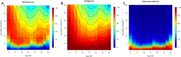
Figure A5. Optimization Surfaces for Skill Score (A), Hit Rate (B) and False Alarm Rate (C) for satellite to airport comparison for varying hours and cloud albedo thresholds. Skill Score is calculated as Hit Rate minus False Alarm Rate. Dashed line denotes cloud albedo of 8.5%.
Download figure:
Standard image High-resolution imageAppendix B. Results and discussion
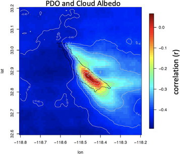
Figure B1. Correlation map of PDO index to 1 km cloud albedo (both are for monthly data May to September) (n = 115).
Download figure:
Standard image High-resolution imageAppendix. B.1. Spatial correlation analysis for cloud variability within SCI
We highlight intra-island structure of the cloud field through the relationship between cloudiness at a point (Eel point) and the rest of the island (figures B2 and B3). High correlations represent locations where cloudiness varies in concert with variations at Eel point. On August mornings, the day-to-day variation in cloudiness is similar across the whole island, but later in the day this is not the case (e.g. at 7 PST all parts of the island are correlated with Eel point cloud albedo r > ∼ 0.65, by 18 PST the correlation has dropped to r ∼ 0.35 in the SE). In May (figure B2) the cloud field varies more similarly from day-to-day throughout the whole island than it does in August (figure B3). Cloud albedo at OP1, in the southeast, is more correlated to Eel point in May than in August, and at 0700 PST than at 1800 PST. The inversion base height (which caps the marine boundary layer and dictates cloud top height) is known to vary seasonally (from sounding measurements in San Diego), with May inversions being higher than in the other months (Iacobellis et al 2010). This seasonal variability in the cloud base helps explain these differences in May and August cloud field structure.
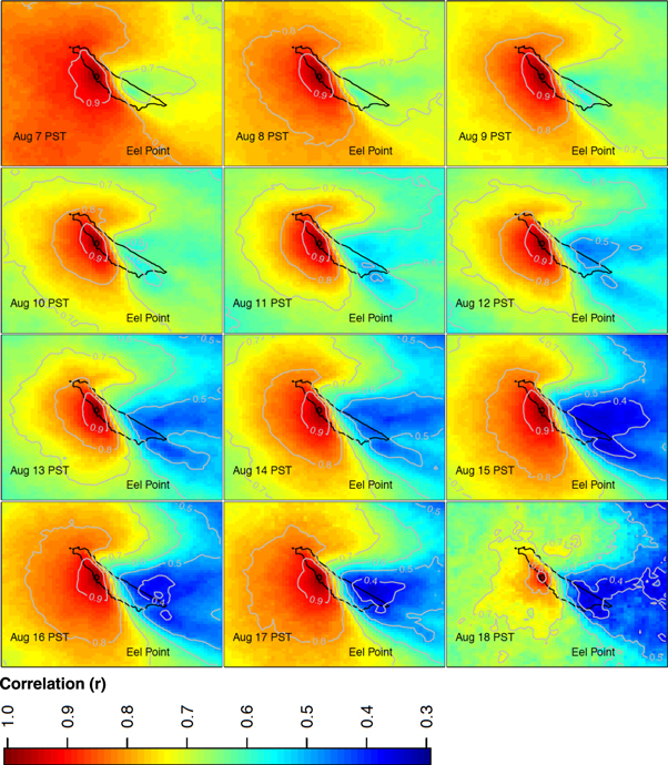
Figure B2. Cloud albedo at Eel Point (black circle) is correlated to cloud albedo at all other 1 km grid cells for August 1996–2018 (23 years). Each panel represents a time from 7 PST to 18 PST. Note these values are correlations (r).
Download figure:
Standard image High-resolution image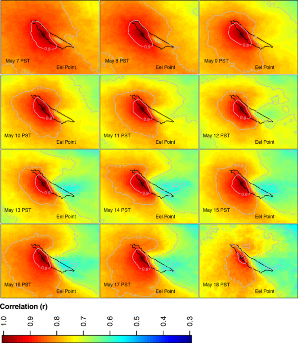
Figure B3. As in figure B2 but for May instead of August and with same color scale. Cloud albedo at Eel Point (black circle) is correlated to cloud albedo at all other 1 km grid cells. Each panel represents a time from 0700 PST to 1800 PST. Note these values are correlations (r).
Download figure:
Standard image High-resolution image