

Abstract
Peatland resilience, defined here as the rate of recovery from perturbation, is crucial to our understanding of the impacts of climate change and land management on these unique ecosystems. Many peatland areas in the UK are managed as grouse moors using small burns (or increasingly, heather cutting) to encourage heather growth and limit fuel load. These small burns or cuts are distinct disturbance events which provide a useful means of assessing resilience. Until now, it has been difficult to monitor the area affected by management each season due to the remoteness and size of moorland sites. Newer satellite sensors such as those on Sentinel-2 are now collecting data at a spatial resolution that is fine enough to detect individual burns or cut areas, and at a temporal resolution which can be used to monitor occurrence and recovery each year. This study considered four areas of moorland; the North Pennines, Yorkshire Dales, North York Moors, and the Peak District. For each of these areas Sentinel-2 optical data was used to detect management areas using the dNBR (differenced Normalized Burn Ratio), and to monitor vegetation recovery using the NDVI (Normalised Difference Vegetation Index). Significant differences were found between the four selected sites in management repeat interval, with the North York Moors having the shortest repeat interval of 20 years on average (compared to 40–66 years across the other three study sites). Recovery times were found to be affected by burn size and severity, weather during the summer months, and altitude. This suggests that the interactions between peatland management and climate change may affect the future resilience of these areas, with hot, dry summers causing longer management recovery times.
Export citation and abstract BibTeX RIS

Original content from this work may be used under the terms of the Creative Commons Attribution 4.0 licence. Any further distribution of this work must maintain attribution to the author(s) and the title of the work, journal citation and DOI.
1. Introduction
Monitoring the resilience of different ecosystems in response to anthropogenic stressors is a topic of growing scientific and policy interest (Côté and Darling 2010). In simple terms, resilience refers to the rate at which a system recovers from perturbations, which is a measure of the strength of feedbacks maintaining a particular stable ecosystem state (or configuration) (Pimm 1984). Loss of resilience can signal the approach to a 'regime shift' where an ecosystem transitions to a different stable state. Peatlands can exhibit alternative stable states, and their resilience to anthropogenic disturbances and climate change is of particular interest, as they are major stores of carbon and can become a significant source of greenhouse gases (Pastor et al 2002, Page and Baird 2016, Harris et al 2020, Lees et al 2021, Milner et al 2021). In the UK, peatlands are projected to be under threat from warming and drying caused by climate change (Gallego-Sala et al 2010, Lees et al 2021). UK peatlands are also already subject to a range of anthropogenic disturbances including deliberate drainage for grazing or forestry (and rewetting to reverse previous drainage), intensive livestock grazing, managed burns and heather cutting (JNCC 2011). Deliberate perturbations can provide a way to measure the resilience (i.e. recovery rate) of an ecosystem (Díaz-Delgado et al 2002, Chambers et al 2019). Fires are particularly promising in this respect as they are temporally and spatially discrete, readily-detectable perturbations.
Many upland peatlands in the UK are managed using small burns to encourage new heather (Calluna vulgaris) growth and thereby create the mosaic of stand ages preferred by red grouse (Lagopus lagopus scoticus). Burn management of peatland is a controversial subject with many areas of the science currently debated (Davies et al 2016a). Post-fire changes in pH, nutrient availability, erosion, hydrology, carbon balances, and vegetation communities have all been observed, but reviews of the literature often prove inconclusive (Tucker 2003, Worrall et al 2010, Grant et al 2012). It is also argued that regular burning limits the fuel load and thereby decreases the potential for large wildfires, although this is contested by others who suggest that a hydrologically restored peatland ecosystem would have a higher water table and a different vegetation community with a lower fuel load (Mcmorrow and Lindley 2006, Marrs et al 2019, Glaves et al 2020). In some areas heather cutting is becoming more widely used as an alternative to burning, although this has raised other concerns (Heinemeyer et al 2019).
Regular burning to encourage heather growth has been a management practice since the early 1800s (Tucker 2003), and estimates suggest that up to 50% of dwarf shrub heath and blanket bog in England and Wales may be managed as grouse moors through regular burning (Worrall et al 2010, Grant et al 2012). Management frequency is difficult to calculate accurately due to the paucity of available data, and spatial and temporal variability of annual burn coverage (Tucker 2003). An oft-cited calculation based on an ideal heather height for burning of 20–30 cm suggests a burn repeat interval of 10–20 years (Tucker 2003, Defra 2007). Estimates based on observations, however, suggest that management frequency is much more variable, ranging from 7 to over 100 years across England (Grant et al 2012, Allen et al 2016).
Aerial photography has previously been used by Allen et al (2016), Thacker et al (2014), and Yallop et al (2006) to map managed burns over small areas. Earlier satellite imagery spatial resolution was too coarse to accurately map the small burns typical of peatland fire management, although burn detection has previously been attempted using MODIS data (Douglas et al 2015). Google Earth imagery has also been previously used to estimate the areal extent of managed burning, but does not have the temporal frequency to map annual burns (Anderson et al 2009, Douglas et al 2015). Newer satellite sensors such as Sentinel-2, however, have both fine scale resolution and a frequent return interval combined with large-scale coverage. The processing power of Google Earth Engine (GEE) enables detailed time series analysis over large areas using these newer fine resolution satellites.
In this study we trial the potential of Sentinel-2 data to map heather management across large managed moorland areas in England, and thereby calculate the managed percentage area and repeat interval at different sites. We also estimate vegetation recovery times following management with Sentinel-2 image series, and consider the factors that may affect the length of post-management recovery. Firstly, we hypothesized that management frequency would have an effect on regeneration period (i.e. resilience), as the management repeat interval affects the dominance of heather in the vegetation community and the stand age before the management (Tucker 2003, Nilsen et al 2005, Davies et al 2010). Secondly, we hypothesized that variations in weather conditions following the burn season, in combination with altitude, could affect recovery rate in different locations, as peatland vegetation needs cool and wet conditions to thrive (Clark et al 2010). Thirdly we hypothesized that burn size and severity would affect recovery times where burning was the management method used, as a larger and more severe fire would potentially destroy the buried shoots of heather which can facilitate regeneration (Tucker 2003). Throughout this article we use the term 'fire severity' to refer to the immediate change in vegetation caused by the burn, following Keeley (2009).
2. Methods
2.1. Selected sites and satellite imagery
Four landscapes which include large areas of managed heather moorland in England were selected; the North York Moors (NYM), Peak District (PD), Yorkshire Dales (YD), and North Pennines (NP) (Anderson et al 2009, Douglas et al 2015). ESRI and Google RGB satellite imagery was used to visually assess areas which showed evidence of recent management in the form of observed burn or cut scars within these landscapes, and shapefiles covering these areas were created in QGIS (QGIS Development Team 2018) (see figure 1).

Figure 1. Map of manually drawn areas with evidence of recent burn management shown in Northern England. Sample areas used in section 2.4.1. are also shown.
Download figure:
Standard image High-resolution imageSentinel-2 satellite imagery processed in GEE (Gorelick et al 2017) was used throughout the study, as it has a spatial resolution of 10 m in the red and near-infrared (NIR) bands, and 20 m in the short-wave infrared (SWIR) bands. It also has a return interval of 2–3 days at the latitudes of our study sites. We used level 1C throughout to maintain consistency, as level 2 data were not available for the earlier years of our study period. We removed all images with a cloud cover percentage of over 60%, and filtered the remaining images for both opaque and cirrus cloud cover using the QA60 band.
2.2. Managed area detection
The differenced Normalised Burn Ratio (dNBR) can be calculated using the NBR from a pre-fire and post-fire image (Key and Benson 2006). The NBR is the normalized difference between a near-infrared band (Sentinel-2 Band 8) and a short-wave infrared band (Band 12) as follows:


Healthy vegetation shows a peak in the NIR range and a trough in the SWIR, but this is reversed in areas affected by fire. The post-fire image is subtracted from the pre-fire image to show the change.
Many previous studies have shown good correlations between the NBR or dNBR and fire severity field measures such as twig diameter and variations of the Composite Burn Index (CBI) in a range of shrubland and grassland ecosystems (Epting et al 2005, Keeley et al 2008, Boelman et al 2011). The dNBR is usually used to assess the severity of single large fires, but we found that it can also be a useful tool for detecting multiple small fires such as those used for managing heather moorland, following Schepers et al (2014) who found that the NBR was the best index for distinguishing between burned and unburned areas, and also had an R2 value of 0.55 when compared to ground measures of severity in heather-dominated heathland. Bare soil and dead vegetation also have lower NIR and higher SWIR reflectance than healthy vegetation, meaning that areas of heather cutting can also be detected by the dNBR. Our results are similar to those recently achieved by Natural England using an alternative method (Natural England 2021).
The burn season is 1st October to 15th April each year (Tucker 2003, Defra 2007), to avoid burning during the summer when the peat is likely to be at its driest and therefore vulnerable to fires getting out of control. To use the dNBR to detect managed burns annually, we selected Sentinel-2 images from the start of the burn season and the end of the burn season (see table 1). For some sites, particularly in 2017, images after the start of the burn season in October were used as the pre-fire image. This could lead to some burns being missed if they occurred at the start of the burn season, but this effect is likely to be minor as most burns occur in the spring. This is due to the gamekeepers being busy during the grouse shooting season which ends in December, and also due to the dead plant matter being drier and easier to burn later in the burn season (GWCT 2021). Where cloud-free images within a month of the start or end of the burn season were unavailable, a cloud-free image further from the burn season start or end date was selected. If there were no completely cloud free images of the area between April and October then several partially cloud-free images were mosaiced together. In some cases it was impossible to find a completely cloud-free image using either of these methods, and so there were small areas of managed moorland which were excluded from analysis in some years.
Table 1. Pre and post burn season image dates. In some cases mosaiced images were used; these are indicated by an asterisk. 2015–16 is shown in figure 2, although not included in the analysis, and the image dates are therefore included for only the NYM.
| Fire season | NYM | PD | YD | NP |
|---|---|---|---|---|
| 2015–16 | 2015-09-30 | |||
| 2016-04-20 | ||||
| 2016–17 | 2016-07-16 | 2016-07-19 | 2016-04-20 | 2016-04-09 to 04–21* |
| 2017-05-05 | 2017-10-27 | 2017-05-25 | 2017-05-04 to 05–26* | |
| 2017–18 | 2017-10-27 | 2017-10-27 | 2017-10-27 | 2017-10-27 |
| 2018-05-27 | 2018-05-05 | 2018-06-24 | 2018-06-27 | |
| 2018–19 | 2018-10-22 | 2018-10-10 | 2018-07-01 to 07-30* | 2018-09-27 |
| 2019-04-22 | 2019-04-17 | 2019-04-19 to 04–26* | 2019-05-12 | |
| 2019–2020 | 2019-10-17 | 2019-09-30 to 10–03* | 2019-10-01 to 10–03* | 2019-10-02 |
| 2020-04-14 | 2020-04-16 | 2020-05-28 to 06–02* | 2020-04-25 to 05–30* |
Where the dNBR is used to assess fire severity for larger wildfires, it is regarded as best practice to select images from the same season pre- and post-fire, and in some cases to select the post-fire image from the year after the fire to include fire-induced mortality in the assessment of severity (Key and Benson 2006, Chen et al 2020). We decided to use images immediately preceding and following the burn season (where possible) instead due to the short repeat intervals between burns, the fast regeneration of moorland vegetation, and the likelihood of pixel overlap where burns in consecutive years were very close together. In these overlapping pixels the vegetation regeneration following an initial burn (causing a negative dNBR) could counteract the fire severity (positive dNBR) resulting from a nearby burn the following year, if the growing season was included in the time period between the pre- and post-fire images.
Once the dNBR was calculated, a threshold value of 0.4 was visually assessed to be the optimum in retaining only management-affected pixels. We found that threshold values of 0.35 or lower included areas of vegetation change along watercourses and in other areas not affected by burning. On the other hand, threshold values of 0.45 or higher missed smaller, less severe burns. A threshold of 0.4 was accordingly used to extract the managed areas for each burn season. High dNBR values not due to moorland management (e.g. field harvesting) were excluded through the use of shapefiles covering the managed moorland areas (see figure 1). Some of the areas detected as burnt areas may actually show vegetation change as a result of heather cutting rather than burns. This is discussed further in section 4, and we have used terms such as 'managed area' and 'management repeat interval' throughout to indicate that some of the detected management may not be burns. As both burns and cutting are employed for the same purpose, we considered it acceptable to include both in this study.
There were appropriate cloud-free images to calculate the dNBR for 2015–16 across the North York Moors (NYM), but not for the other three sites due to there being fewer images in that period before the second Sentinel-2 satellite had been launched. The 2015–16 dNBR for the NYM is therefore shown in figure 2, but is excluded from all other analysis to allow fair comparisons with the other three sites.

Figure 2. Detected burns in the fire seasons beginning 2015 to 2019, on an area of the North York Moors (westernmost sample area as shown in figure 1). If there is an overlap the most recent year is shown. The blue point marker shows the point used to give the graphs in figure 3.
Download figure:
Standard image High-resolution imageManagement coverage and frequency were calculated following Yallop et al (2006) who estimated burn repeat intervals by calculating the percentage of managed moorland area which was burnt each year. Using QGIS we created a grid of 500 m by 500 m squares within the managed moorland polygons, and used these grid squares to calculate percentage area managed for each year. Management repeat intervals in years were then calculated by estimating how long it would take for the whole area to be subject to management if the average percentage managed area remained constant (see figure 5). A 500 m grid was selected as the optimum grid size as smaller grid sizes (100 m) were of similar size to individual areas of management, and larger grid sizes (1 km) would in some cases have had different management styles within grid cells, thereby losing some of the spatial variation.
2.3. NDVI recovery rate
The Normalised Difference Vegetation Index (NDVI) is the normalised difference between the red band (Sentinel-2 Band 4) and the near infrared (Band 8A) as follows:

The NDVI detects vegetation health and coverage, and has been successfully used to measure fire recovery in shrubland (Malak and Pausas 2006, Hope et al 2007, Sankey et al 2013, Ireland and Petropoulos 2015, Storey et al 2016) and wetland ecosystems (Potter 2018, Sinyutkina et al 2019). First the NDVI sequence from June 2015 (when the first Sentinel-2 satellite was launched) to the end of 2020 was calculated from Sentinel-2 Level 1C data. This dataset was averaged over each of the managed moorland areas (see supplementary material (available online at stacks.iop.org/ERC/3/085003/mmedia) for further details of why this method was used), and smoothed using an average of the images within 20 days of each DoY (Day of Year), to give an average annual cycle. A 20-day window was used to capture the full seasonal range whilst removing most of the noise from the cycle. This average annual cycle was then subtracted from the NDVI values for each burnt pixel, from the 16th April following the burn season to the end of the year. The residuals were smoothed using a 20-day moving average, and the time taken for these residuals to reach zero (i.e. to recover to the average seasonal cycle) was then calculated (see figure 3). If the NDVI residuals had not reached the average seasonal cycle by the end of the year, i.e. after 259 days, the recovery period was automatically set to 260 days.
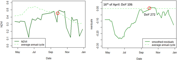
Figure 3. Graphs showing the NDVI recovery calculations for point -1.02409, 54.41982 (WGS84, see figure 2) on the NYM which was burnt in the 2017–2018 burn season (this graph therefore shows data from 2018). The recovery time is 166 days (the difference between the 16th of April and the cross-over point).
Download figure:
Standard image High-resolution imageA two-way ANOVA followed by Tukey HSD statistical analysis was used to consider the differences between recovery times across the four sites and the four years which had useable data from all sites (2016–17; 17–18; 18–19, 19–20). All statistical analysis was completed in RStudio (R Core Team 2019).
2.4. Factors affecting recovery times
Management frequency, fire severity, weather conditions, and altitude were assessed as potential factors affecting recovery times. Fire severity was assessed using the results of the dNBR datasets which were initially used to detect the burns (see section 2.2.).
To test whether climatic conditions had an effect on recovery timescales, the ERA5 reanalysis dataset was used (Munoz Sabater 2019). Following Clark et al (2010) we hypothesised that water availability and temperature were likely to be the most important weather factors. We therefore downloaded mean 2 m air temperature and total precipitation data for the study sites. Data averages across the moorland areas were used for longer-term site comparisons, and preliminary analysis in comparison to recovery results. This preliminary analysis suggested that summer (JJA) weather had the greatest impact on recovery times, and ERA5 datasets at the original spatial resolution of 0.25 arc degrees covering this period for each year were therefore downloaded and analysed by extraction using the grid. To test the effect of altitude, SRTM (Shuttle Radar Topography Mission) 1 Arc-Second Global dataset was downloaded from USGS for the four sites. This 30 m resolution elevation data was then extracted using the grid.
All variables were correlated using the Corrplot package (Wei & Simko 2017). Multiple linear regressions were used to assess the significance of the factors affecting recovery times, and interactions between factors were included in the models to determine the R2 values. Weighted Least Squares (WLS) was used where the initial model residuals were non-normal. All statistical analysis was completed in RStudio (R Core Team 2019).
2.4.1. Individual fires analysis
We hypothesized that fire size is a large factor in both severity and recovery. It was challenging, however, to develop a method to measure fire size, as the resolution of the satellite data often caused burns close to one another to be conflated into a single fire if only a threshold value was used (see figures 2 and 10). We therefore decided to undertake a smaller case study on three areas of the NYM and manually outline individual fires using visual assessment of the dNBR and RGB imagery. This smaller case study also alleviates potential concerns about comparing fire severities calculated using different images (Chen et al 2020), as all three areas selected were within the same satellite images for calculation of the dNBR.
The individual burns to manually detect were selected by drawing three rectangles over areas of the NYM following the 2017–18 fire season (the NYM was selected due to the high density of managed burns, and the 2017–18 season was selected due to the longer recovery times in that year—see section 3). The three rectangles were drawn in areas where there were many burns of different sizes and severities apparent (see figures 1 and 2). The burnt areas were manually detected and converted to shapefiles, and the average and maximum severity and recovery time for each fire were then extracted. The area of each burn was calculated using QGIS, and the area was also divided by the perimeter to give a variable we have named 'shape'. This variable distinguishes between fires which are more circular in shape, and those which are elongated (see figure 10). All these variables were correlated using the Corrplot package (Wei and Simko 2017). Multiple linear regressions were then used to assess the significance of the factors affecting recovery times, and interactions between factors were included in the models to determine the R2 values. Weighted Least Squares (WLS) was used where the initial model residuals were non-normal. All statistical analysis was completed in RStudio (R Core Team, 2019).
3. Results
3.1. Management occurrence and frequency
The percentage areas managed are different between sites, but also vary year to year (table 2 and figure 4). The average management repeat interval was found to be shortest on the NYM (20 years), followed by the YD (40 years), then the PD (45 years), with the NP having the lowest percentage area managed each year, and the longest repeat interval (66 years). A one-way ANOVA on the average managed area percentages showed that all sites apart from YD and PD were significantly different. The results shown in table 2 and figure 4 appear different because table 2 shows the percentage area managed and repeat intervals calculated across the whole of each moorland area, whereas figure 4 shows the ranges of the repeat intervals for each of the grid squares within the moorland areas. Some repeat intervals appear unrealistically high (>100 years) due to grid squares where very few pixels were burnt during the four-year study period.
Table 2. Managed area statistics for the four areas. The individual burn seasons are given as percentage managed area, the total is given as the overall repeat interval calculated using the four burn seasons.
| Burn season | North York Moors (NYM) | Peak District (PD) | Yorkshire Dales (YD) | North Pennines (NP) |
|---|---|---|---|---|
| 2016–17 | 6.67% | 1.58% | 0.23% | 0.62% |
| 2017–18 | 2.11% | 3.44% | 1.53% | 0.51% |
| 2018–19 | 4.32% | 1.06% | 5.59% | 3.95% |
| 2019–20 | 6.92% | 2.88% | 2.70% | 0.94% |
| Total management repeat interval | 19.99 years | 44.69 years | 39.81 years | 66.42 years |
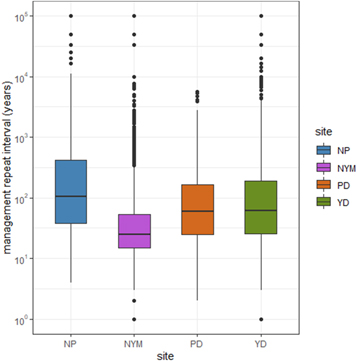
Figure 4. Box plot of the differences in management repeat intervals between the four managed moorland sites, shown on a log scale. Each point is a grid square (n = 1537, 1927, 439, 2082).
Download figure:
Standard image High-resolution imageThe large spatial variation in management repeat intervals across the four sites is also worth noting (figure 5). Some grid squares had high percentage management coverages in several years of the study, and therefore calculated management repeat intervals of less than ten years.
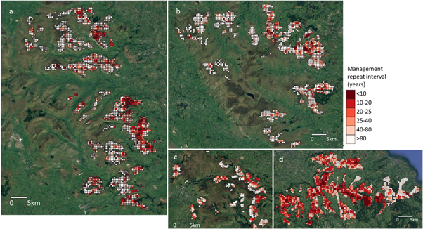
Figure 5. Management repeat intervals over (a) the Yorkshire Dales, (b) the North Pennines, (c) the Peak District, and (d) the North York Moors.
Download figure:
Standard image High-resolution image3.2. NDVI recovery rates
NDVI recovery rates also varied between years and sites, and within sites (figures 6 and 7). The results of the two-way ANOVA showed that both year and site had a significant effect (p < 0.001) on recovery times, and that the interaction between year and site was also significant (P < 0.001). The Tukey HSD post-hoc testing showed that the recovery times for all four years were significantly different, and that all the sites were significantly different to each other. The linear model including site and year gave an adjusted R2 value of 0.28 (p < 0.001).
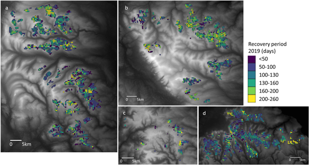
Figure 6. Mean recovery rates across (a) the Yorkshire Dales, (b) the North Pennines, (c) the Peak District, and (d) the North York Moors in 2019, displayed on the SRTM digital elevation data.
Download figure:
Standard image High-resolution image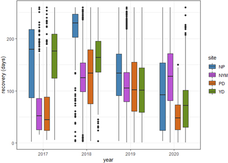
Figure 7. Box plots showing the differences in mean NDVI recovery period (days from 16th April) for the grid squares within each of the four managed moorland sites across the four years of the study period.
Download figure:
Standard image High-resolution imageRecovery times were generally longer in 2018 than in the other years of the study. The NP and YD had longer recovery times than the NYM and PD in general, although this varied between years (figure 7).
3.3. Factors affecting recovery times
A multiple linear regression model combining all factors (severity, average percentage managed area, altitude, precipitation, temperature, year, and site) showed that all factors were highly significant (p < 0.001) except percentage managed area (p < 0.1) and altitude (not significant). Table 3 shows the results of the linear models used to analyse the strength of influence of each of the factors on the recovery times, and figure 8 shows the correlations between factors. The model containing all factors had the highest R2 value of 0.42. Year was the most influential factor, followed by site, as these have comparatively higher R2 values when modelled independently (0.097 (0.11) and 0.052 respectively) and removing them from the total model has the greatest impact (R2 values of 0.28 and 0.33 respectively). The other factors are all relatively similar in terms of their explanation of variance, apart from percentage managed area which has minimal effect, and they all add in small but significant ways to the overall model, as shown by the reduced R2 value when each is removed (see table 3). Further investigation into the high R2 value of percentage managed area when using WLS revealed that a few fragments of grid cells with unrealistically high percentage managed areas (>20%) were having a disproportionate impact on the model. When these were removed the model was no longer significant and explained almost no variance.
Table 3. Linear models showing the impact of the different factors affecting recovery. Numbers in brackets show values for Weighted Least Squares (WLS) models where the residuals of the original model were non-normal and WLS improved the fit.
| Model factors affecting recovery | Adjusted R2 | p-value |
|---|---|---|
| Severity | 0.0027 (0.087) | 0 |
| Percentage managed area | 0.00033 (0.14) | 0.02 (0) |
| Altitude | 0.013 | 0 |
| Precipitation | 0.041 (0.045) | 0 |
| Temperature | 0.0035 | 0 |
| Year | 0.097 (0.11) | 0 |
| Site | 0.052 | 0 |
| All factors | 0.42 | 0 |
| Factors apart from severity | 0.37 | 0 |
| Factors apart from percentage managed area | 0.41 | 0 |
| Factors apart from altitude | 0.38 | 0 |
| Factors apart from precipitation | 0.39 | 0 |
| Factors apart from temperature | 0.39 | 0 |
| Factors apart from site | 0.33 | 0 |
| Factors apart from year | 0.28 | 0 |

Figure 8. Correlation plot of the factors affecting recovery. Blank squares show correlations that are not significant at the 99% level. Darker colours and larger squares show stronger correlations; blue shows positive correlations, red shows negative.
Download figure:
Standard image High-resolution imageThe JJA precipitation across the study period clearly shows that 2018 had much lower summer rainfall than the other years, and the JJA temperatures of 2018 were also slightly higher than those of the other three years (figure 9). Precipitation and temperature have a negative correlation of −0.68 (figure 8), as higher temperatures are associated with lower rainfall in the summer.
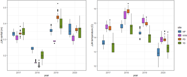
Figure 9. JJA total precipitation and average temperature over the four years of the study. Data from ERA5.
Download figure:
Standard image High-resolution image3.3.1. Individual fires analysis
Individual fires were manually detected from three areas on the NYM following the burn season 2017–2018 in order to analyse the effects of fire size and shape (figure 10). The burn sizes across the three sample rectangles ranged from 365 to 27,823 m2; 211 to 8,889 m2; and 364 to 18,249 m2, with means of 3,859 m2 (0.39 ha), 1,921 m2 (0.19 ha), and 2,499 m2 (0.25 ha) (for sample rectangles west to east respectively).

Figure 10. Westernmost sample square as shown in figures 1 and 2 showing burns in the 2017–18 burn season. Clockwise from top left the images show: burn severity calculated using dNBR; grid square management repeat intervals as shown in figure 5; grid square and individual burn recovery times as shown in figure 6; burn shapes.
Download figure:
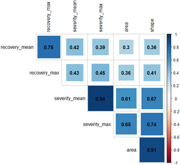
Standard image High-resolution imageFigure 11 shows a correlation plot of fire size, shape, severity, and recovery. Both severity and recovery are positively correlated with area and shape, and the strongest correlations in each case are between maximum values and fire shape (0.74 and 0.41 respectively). This indicates that larger, more circular fires have higher severities and take longer to recover. There is also a positive correlation between fire severity and recovery time (0.45 between maximum values).
Figure 11. Correlation plot of the individual fire variables. All correlations are significant at the 99% level. Darker colours and larger squares show stronger correlations; blue shows positive correlations, red shows negative.
Download figure:
Standard image High-resolution image
A multiple linear regression model analysing the impacts of the factors (severity mean and max, area, and shape) on the mean recovery showed that mean severity and shape were significant (<0.01) whilst maximum severity and area were not significant.. The R2 value of the linear model including all factors and interactions was 0.18, and remained the same when only mean severity and shape were included. When a multiple linear regression model was fitted for maximum recovery only the maximum severity was significant (p < 0.05). The R2 value of the linear model including all factors and interactions was 0.23, and 0.20 when only maximum severity was used. A multiple linear regression model analysing the impacts of area and shape on severity showed that only shape was significant (p < 0.001) in relation to both mean and maximum severity, and the linear model using only shape gave an R2 of 0.45 for mean severity (0.40 using WLS) and 0.54 for maximum severity (0.50 using WLS).
4. Discussion
4.1. Management occurrence and frequency
We found that management frequencies varied greatly between and within the four moorland study areas used in this work. The averages across the four sites gave management repeat intervals ranging from 20 to 66 years, but within the sites some areas were found to have repeat intervals of less than ten years.
Yallop et al (2006) used aerial imagery collected in 2000 to calculate that approximately 4% of managed heather moorland area in England was burnt each year, and the average repeat interval was approximately 20 years. The results from the NYM in the current study give very similar results, with 5% being managed per year on average over the four-year study period, and therefore a repeat interval of 20 years. The other three sites, however, show lower management percentage areas and therefore longer repeat intervals. Following a similar method to Yallop et al (2006), Thacker et al (2014) found a repeat interval of 26.6/25.1 years (deep peat/other soils) in England, with 11.3/13.8 for the NYM, 19.8/21.2 for the YD, 23.7/27.0 for the PD, and 28.0/26.3 for the NP. They used aerial imagery from years 1999–2009, but coverage was not complete over all sites. These results agree with our study in the order of most frequent to least frequently managed over the four areas, but suggest shorter repeat intervals. Using satellite data allows much larger areas to be assessed, and also has a much more frequent return interval, allowing individual years to be considered rather than a visual estimation of burn scars.
Allen et al (2016) found a rate of only 0.9% (0.7%–2.4% of the 'potentially burnable' area) per year on Howden Moor in the Peak District, giving repeat intervals of 42–142 years. However, they also noted that 13% of burnt area during the study period had been burnt less than 10 years previously (the actual figure was likely to be higher due to the limitations of the 21-year study period), and that some areas were burned five times during the period. This suggests that the frequency of management is not even, with some areas being burnt very frequently and some very infrequently, and agrees with the results from our gridded datasets which show repeat intervals ranging from less than 10 years to more than 80. Our results show that 11.1% of the NYM area with evidence of heather management had repeat intervals of ten years or less, but across the PD this was only 1.1%. This estimate is much lower than Allen et al's (2016) 13%, but includes areas which were not managed at all during our study period. Allen et al's (2016) study covered a much smaller area over a longer time period, ensuring that areas with burn management were accurately defined. In contrast, the current study relied on a cruder visual estimation of management areas from RGB imagery from a limited date range. Over the area of Howden Moor used in Allen et al's (2016) study, only some of the areas of burn management shown in their work were included in our method, and the areas we included showed repeat intervals of 16–980 years. Applying our method over longer timescales would improve the reliability of repeat interval estimates, although changes in management regimes between different study periods are also a factor (Thacker et al 2014).
The differences between sites and years may be partly due to image selection, as in some cases there were no cloud-free images available within a month of the start or end of the burn season. In these cases, images further from the burn season, mosaiced images, or images with minor cloud cover were used. A longer gap between pre- and post- images may have caused only more severe fires to be detected, as less severe fires may have been obscured by the natural changes in vegetation over the seasons (Chen et al 2020), whilst using images with some cloud cover may have led to a slightly lower burned area percentage. Using data from multiple years helped to minimise the potential effects of image selection in calculating the differences between sites. Another potential concern was that the fire severity calculated by the dNBR can vary depending on the vegetation structure and phenology of the site, and previous studies have used adaptive thresholding rather than a specific value to overcome this (Chasmer et al 2017, Chen et al 2020). We considered this a minor issue in our use of the dNBR however, as the areas used in this study were all heather-dominated managed moorland, and so we made the assumption that they have similar vegetation.
This study was limited by the short time period of available data, with only four years with imagery suitable to calculate the dNBR and the recovery rate for all four managed moorland sites. This may lead to some misrepresentation of management repeat intervals at individual grid squares, as areas where large areas were subject to management in the years preceding the study might not have been managed so heavily during the period when imagery was available, leading to a lower repeat interval. Conversely, areas which were only minimally managed in the years preceding, but where large areas were subject to management during the study period, may have a falsely high repeat interval.
Weather conditions through the burn season have a large impact on the percentage land area which can be burnt each year, as wet weather can make the vegetation difficult to ignite, snow cover can prevent burns, and high winds can increase the risk of fires getting out of control (Tucker 2003). In the early part of 2018, for example, there was unusually heavy snowfall across much of the UK, which would have prevented burning during this period. This can be seen particularly well in the 2017–18 burn season on the NYM, where the percentage burnt was only 2.1% compared to the average of 5%. In contrast, the area managed on the YD and NP appears to have been particularly high during the burn season of 2018–19, perhaps due to the warmer weather in the early months of 2019.
In recent years heather cutting has become an increasingly popular alternative to burn management (Heinemeyer et al 2019). Our method using dNBR thresholding may in some cases mis-identify heather cutting as (lower severity) burns due to the change in vegetation, and there is a need for further work to develop remote sensing methods that can distinguish between these management methods. The inclusion of heather cutting areas in the study may also have had some effect on recovery times (see below).
Our developed method for detecting burns using high resolution satellite data is useful for gaining overviews of heather moorland management rapidly and remotely. We hope that this technique will be useful for land managers mapping and monitoring management locations and repeat intervals, and for researchers seeking to analyse changes in management across moorland areas.
4.2. Management recovery rate
We hypothesised that management frequency, weather, altitude, and fire size and severity would all affect vegetation recovery times. The results explored in section 3.2 can support most of these hypotheses, although the interactions between them are complex. Additionally, the differences in recovery times between the four selected sites are not fully explained by these factors alone, and it is likely that there are other factors playing a role such as stand age (Nilsen et al 2005, Davies et al 2008), slope aspect (Ireland and Petropoulos 2015), heather beetle damage (Rosenburgh and Marrs 2016), pollution levels or grazing densities (Milner et al 2021).
The recovery times shown in the results of this study should not be taken as absolute values; that is, it should not be assumed that the vegetation of a managed area is likely to recover completely within a year from the end of the burn season, although the greenness may recover quickly due to young heather shoots and fast growing species such as grasses and bilberries. The NDVI is also far more sensitive to horizontal vegetation spread than vertical growth with age (Storey et al 2016). In reality, fire scars can be seen on the landscape for several years after a burn, and vegetation communities can be different even when the NDVI recovers (Noble et al 2018, Grau-Andrés et al 2019). Noble et al (2019) found that on many sites one-year post-burn there was high vegetation cover and few areas of bare peat, suggesting that recovery in terms of greenness is plausible on such short timescales. Similarly, Grau-Andrés et al (2017) showed that the photosynthetic capacity of fire-affected Sphagnum capillifolium recovered after less than two years. Nilsen et al (2005) studied burn-managed heather specifically, and noted that percentage cover reached up to 50% after one year. Sinyutkina et al (2019) found that NDVI and vegetation of a drained bog in West Siberia recovered two to three years post-fire. This was a larger and most likely more severe fire than managed burns, however. It must also be considered that the small size of many areas of management relative to the size of the Sentinel-2 pixels means that the NDVI of detected managed areas is likely to also include some edges where there was still untouched vegetation, as well as areas within the managed area where some vegetation survived. The results displayed in figures 6 and 7 are averages of whole grid squares, which include small, fast-recovering management areas, as well as larger burn scars which may take longer than a year to recover. There may also be areas where fires earlier in the burn season (October) could already have seen some vegetation recovery by the end of the burn season (April) (Sankey et al 2013), although we assume this effect to be minimal given that most recovery is likely to occur during the spring and summer growing season. A different vegetation index, or combination of indices and other remote sensing data, might give more accurate recovery timescale results, but validation with ground data is needed.
The method used to calculate the seasonal NDVI cycle has an impact on the resulting recovery times, and was therefore carefully considered. The four different managed moorland areas selected in this study have similar seasonal cycles, with the NP having the highest summer peak in NDVI at 0.56, and the YD the lowest at 0.53. We decided to include the recently managed areas in the calculation of the seasonal cycle in order to get a complete picture of the moorland area (see supplementary material for further explanation). Given the assumptions made in the calculation of the seasonal cycle, it is important to stress that the recovery times used in this study are an estimate of the resilience of each site in its current state. The longer recovery times of the NP, for instance, may be partly a result of the vegetation communities across those sites having a lower resilience to disturbance. The inclusion of some areas of heather cutting may also affect the recovery times of areas where this method is becoming more popular and the use of managed burns is decreasing. Future work could use this method to compare areas of managed burns to areas of heather cutting to assess the recovery times of each, which could add to our understanding of the pros and cons of each management strategy.
The weak relationships between recovery and percentage managed area suggest that management frequencies (repeat intervals) have limited impact on recovery times. This is a somewhat surprising result, as it had been hypothesised that a higher management frequency would mean lower stand ages and therefore faster recovery (G.M Sedláková and Chytrý 1999, Nilsen et al 2005, Davies et al 2010, Davies et al 2016b). It may be the case that the impact of stand age on recovery times is limited by other factors also affected by management frequency, such as changes in the vegetation community. It is also likely that the correlation between percentage managed area and severity (see figure 8) impacts on the relationship between management and recovery, as areas with larger fires will have higher management percentages, and are also likely to have higher average severities.
The calculated recovery times have significant relationships with weather conditions, particularly summer rainfall, agreeing with Clark et al (2010) who found that peatland areas are more vulnerable where maximum summer temperatures are higher and annual moisture availability is lower. The differences in summer weather conditions between sites and years contributed to the differences observed in recovery times (figure 7), such as the summer of 2018, when the summer was hot and dry and recovery times were longer (see figure 8). More detailed statistical analysis of the relationships between recovery and weather is needed, but is currently limited by the short duration of the satellite data available, and by the coarse spatial resolution of the ERA5 dataset. It is likely that the relationship between weather and resilience is more complicated than a simple linear relationship with summer rainfall and temperature, as indicated by the difference in recovery times between the years of the study period which was not fully explained by the precipitation and temperature data included in the model. Previous studies have found that drought can have long-term impacts on peatland vegetation (Lees et al 2019), and it may be the case that vegetation recovery times are affected by preceding weather conditions as well as patterns in the summer following management. The positive relationship between altitude and recovery times indicates that factors such as growing season length and exposure to higher winds may also have an impact.
Manual detection of individual fires showed fairly strong correlations between fire size, severity, and recovery. The shape of the burn also had an impact, with larger, more circular burns having higher severities, and in particular higher maximum severities at the centre of the burnt area. It must be noted, however, that this may be partly a result of the satellite pixel size, which includes some unburnt vegetation in the edges of the managed areas. Higher fire severity has previously been associated with larger burn sizes, particularly burns wider than 30 m (Tucker 2003). There are limitations to using this method of individual fire analysis, including the difficulty of visually distinguishing between small, clustered burns. There is also the potential for large burns of lower severity to be missed or to appear smaller than they truly were, as the threshold value of the dNBR used to detect fires may mean that very low severity areas are excluded from analysis. This potential issue was minimised by visually comparing threshold-selected images of burns with the raw dNBR data for the whole area, and also RGB imagery, to consider patterns. Machine learning object detection methods, such as regional convolutional neural networks, could help to minimise user error. Machine learning would also enable larger volumes of data to be analysed cost-effectively, especially as finer resolution optical images become available. Fire recovery times, especially maximum recovery times, were related to the severity of the burn, and therefore to fire size and shape. Higher fire severities can destroy buried shoots, thereby affecting the regeneration period (Tucker 2003). Grau-Andrés et al (2017) found that photosynthetic capacity in Sphagnum capillifolium was lower following higher severity fires, but recovered at the same pace as areas affected by lower severity fire, whilst Davies et al (2010) showed that heather regeneration is highly dependent on stand age preceding the fire, and only minimally affected by fire severity. The current study adds to our knowledge of the effect of fire severity on peatland vegetation regeneration by suggesting that higher severity fires may take longer to recover, but that other factors also play an important role. There is potential for future studies to consider in more depth the relationships between managed burn size, severity, and recovery, which could have important management implications regarding recommended burn sizes.
There is a need for further studies to compare ground data with remote sensing measures of fire severity and management recovery. Previous studies have shown that the methods used in this article are viable for estimating severity and recovery in these environments (Schepers et al 2014, Sinyutkina et al 2019), but there is still work needed on the detail of these relationships. In particular, research comparing the range of field measures of fire severity to the dNBR and other severity indices, and comparing recovery in vegetation cover, height, and species composition to NDVI and other vegetation indices, would be very useful for reliable application of these methods. Comparison between field and remote sensing data over longer-term recovery of post-fire vegetation communities spanning several years would be especially useful. Future studies could also consider combining Synthetic Aperture Radar (SAR) or Light Detection and Ranging (Lidar) data with Sentinel-2 optical data to study management recovery (Chasmer et al 2017). Stand-age has previously been found to affect recovery of managed heather moorland, and there is the potential for SAR or Lidar data to be used to estimate stand-age (Davies et al 2010, Grau-Andrés et al 2019). In the case of SAR data, however, there are complex interactions between surface roughness and soil moisture content (Zhou et al 2019, Lees et al 2021) which would require comprehensive post-fire ground truthing to analyse accurately. Future work should also consider the interaction of managed burns with wildfire and the effect of limiting the fuel load by regular burning or cutting. At the time of writing there have not been enough wildfires on managed moorland during the period covered by Sentinel-2 data for this to be studied in depth.
The results of this study have implications for moorland management. The heather and grass burning code (Defra 2007) recommends avoiding burn repeat intervals of less than 10 years, especially on deep peat. It also recommends smaller burns with a maximum width of 30–55m and an area of less than 2ha (20,000m2), and our results provide further evidence that larger fires are detrimental to the resilience of moorland ecosystems. Our findings regarding the impacts of weather on resilience suggest that the impacts of climate change, especially on summer rainfall, should be taken into account in decisions on how to manage upland peatlands in the future.
5. Conclusions
This study has demonstrated the potential of finer resolution satellite sensors such as those of Sentinel-2 to monitor management frequency and vegetation regeneration on managed heather moorland. Remote sensing is becoming more widely used amongst conservation practitioners in peatland landscapes, and this work provides further evidence of the value of satellite data in monitoring these large and remote ecosystems.
Using satellite data allowed us to compare the four selected study sites and consider the variations in management coverage and frequency between them. This would have been difficult and costly to achieve using aerial imagery, and provides valuable new information on management frequencies across England. Our results show that the North York Moors had shorter management repeat intervals than the other three sites, but that the vegetation recovery times varied widely between sites and years.
Sentinel-2 NDVI time series provide an efficient way to estimate vegetation recovery following management. We found that recovery times were affected by weather, particularly summer rainfall when peatland areas can be susceptible to drought. Altitude also played a role, as vegetation in higher areas recovered more slowly. Regeneration was also affected by fire severity, with larger and more severe fires taking longer to recover fully. These results add to our growing knowledge of the effects of management on heather moorland, and suggest potential interactions with ongoing climate change. Recovery rates can be used as a resilience indicator, suggesting that areas where summer weather is becoming hotter and drier may lose resilience in the future. This agrees with previous studies (Clark et al 2010, Gallego-Sala et al 2010), and indicates that management in peatland areas could be adapted to limit future vulnerability.
Acknowledgments
Thanks to the three anonymous reviewers for their comments which helped to improve this manuscript.
Data availability statement
No new data were created or analysed in this study.
Funding
K Lees, T Lenton, C Boulton & J Buxton were funded by Leverhulme grant no. RPG-2018–046.