


Abstract
Energy policy and investment are commonly informed by a small number of scenarios, modelled with proprietary models and closed data-sets. It limits what levels of insight that can be derived from it. This paper overcomes these critical concerns by exploring a large number of scenarios with an open-data and open-source model to address regional mitigation policy. Focusing on South America, we translate an ensemble of long-term electricity supply scenarios into policy insights and use post-processing methods to present a systematic mapping of solution outputs to model inputs. We find demand levels, the cost of capital and the level of CO2-limits to be significant determinants of total investment cost. Low-carbon pathways are associated with low demand and low cost of capital. When cost of capital increases a shift away from wind and hydropower to natural gas and solar PV is seen. We further show that appropriate concessionary finance together with energy efficiency measures are critical—at a continental level—to unlock economic, low-carbon investment.
Export citation and abstract BibTeX RIS

Original content from this work may be used under the terms of the Creative Commons Attribution 3.0 licence. Any further distribution of this work must maintain attribution to the author(s) and the title of the work, journal citation and DOI.
Introduction
Investment in low-carbon energy is a central topic to low- and middle-income countries' development policy. This is recognised by the United Nations' 2030 Agenda for Sustainable Development that highlights that two of its 17 Sustainable Development Goals (SDG) should be dedicated to, respectively, the provision of affordable and clean energy for all (SDG7) and the imperative of climate action (SDG13) (UN General assembly 2015). SDG 7 was the focus of the High Level Political Forum (HLPF) held in New York in 2018. Further, the 2015 Paris agreement targets a global development path that keeps temperature rise to well below 2 degrees Celsius above pre-industrial levels (UNFCCC 2015). Within this framework, most countries have submitted nationally determined contributions (NDCs), all of which include mitigation measures in the energy sector. Most countries, however, still need to understand the implications that their plans carry in terms of technology choice, timing of investment, and total system cost.
Overcoming the lack of scrutiny that can be associated with the analysis that underpins energy infrastructure development is crucial to unpacking future energy investment decisions. As Pfenninger (2017) points out, key analysis that informs energy strategy in the United States is obscure. In Europe, similar analysis has simply been called 'closed' (Clark 2011). In this paper, we propose a transparent method to inform South American electricity investments by 2050 that relies on generating several hundred scenarios and applying a scenario discovery method.
South America has almost closed its energy access gap with 90% of the population having electricity connections in Bolivia and Peru and almost 100% having access elsewhere (World Bank, WDI 2016). The carbon intensity of the electricity sector in South America is the lowest in the World. Paraguay produces 100% of its electricity from hydropower. This share is above than 60% in Brazil, Venezuela, Colombia and Uruguay (World Bank, WDI 2016).
Notwithstanding, the energy sector in South America could be at a turning point (Elizondo Azuela et al 2017). Demand is increasing due to rapid urbanization and a growing middle class. Though it remains high, the share of electricity produced from hydropower has declined in recent years through drought and poor water resource management. Further, hydropower expansion in the region may be difficult due to mounting opposition to new large-scale projects (Fay et al 2017).
Future energy supply system configurations are uncertain. Selected climate scenarios have implied that lower rainfall could lead to reduced water flow, decreasing the ability of existing and any new hydro investments to generate power. For new hydro (and other capital intensive power plants), the cost of capital will influence the optimal energy investment mix. A high cost of capital makes capital-intensive power plants harder to finance (Schmidt 2014) and therefore relatively less attractive. In parallel other renewable energy technologies (RET) are experiencing high learning rates and have correspondingly falling costs, reducing the appeal of conventional RET such as hydro. All RET technologies stand to benefit from GHG mitigation policies such as carbon taxes and emission caps. It is however unclear how such policies would be configured and whether they would endure.
These considerations, together with institutional, behavioural and social uncertainties, all influence the penetration of low-carbon technologies (Iyer et al 2015a). This in turn impacts the competitiveness of other technologies and affects investment decisions in energy supply. Nevertheless, investment decisions must be made. To understand the influence of one or more of these uncertainties on decision making this paper develops and models scenarios that reflect uncertainty through changes in key input parameters. Recognising that uncertainties are diverse and often non-exclusive, scenarios with different changes need to be combined. This can lead to increased numbers of scenarios, making tractable insight difficult to internalise and communicate. Though easier to digest, a limited number of scenarios makes it difficult to assess whether the most important parts of the solution space are accounted for (McJeon et al 2011).
To address this, we move away from traditional scenario development and use a 'scenario discovery' approach (Bryant and Lempert 2010, Rozenberg et al 2014a). A large set of scenarios is designed using ranges of selected input parameters, or determinants. These scenarios are assessed using key metrics, or attributes. The relations between important attributes and their determinants are then post-processed with data-mining tools that help to decipher the multidimensional solution space. Further, the data, model and methods are all transparent and open source6 . This ultimately allows for complete repetition of the experiment and for policy transparency. To our knowledge, it is the first time that open-source approaches and the scenario discovery methodology have been combined for South America. Extending this work outlines a future where complexity can be deciphered and policy support can be scrutinised.
Method
Model description
The energy system is both strategic and capital intensive. Policies and development support therefore need to be easy to audit and review. Because energy infrastructure outlast any electoral or administrative cycle, such transparent information is critical for stakeholders including the public, that is, taxpayers and voters, and support organisations, like development banks. To this end, the analysis uses the Open Source Energy MOdelling SYStem (OSeMOSYS) which is an open source energy model generator that uses linear optimization techniques, and has global application (Fattori et al 2016, Löffler et al 2017, Niet et al 2017, Pfenninger et al 2018, Taliotis et al 2016, UN DESA 2016). It determines the cost-optimal long-term investment and operation required to satisfy an exogenously defined energy demand (Howells et al 2011). It overcomes recent criticism levelled at similar energy systems models that are not open. Pfenninger (2017) argues that lack of transparency, stemming from lack of open source methods leads to lack of trust in analysis. Yet trust and transparency will be needed to address future long-term low-carbon investment trajectories.
For the same reasons, this paper uses the OSeMOSYS-generated South AMerica Model BAse (SAMBA): an open-source, open-access, long-term, integrated electricity sector model. It explicitly represents eleven South American countries: Argentina, Brazil, Bolivia, Chile, Colombia, Ecuador, Guyana, Paraguay, Peru, Uruguay and Venezuela. Each country is included as an individual region except for Brazil, which is represented using four sub-systems (ONS 2015). The final model has fourteen regions and a time horizon spanning 2013–2063 in one-year time-steps.
SAMBA includes a wide range of technologies, which are represented on a national level. These comprise renewable, nuclear and fossil-fuelled technologies. Hydropower storage is included in the four sub-regions of Brazil and in Venezuela; a detailed list is included in appendix A—table A1. An early application of SAMBA can be found in (de Moura et al 2017 and de Moura et al 2018). Changes as implemented for this project can be found in appendix A—table A2.
Electricity trade between countries relies on the 21 existing international interconnection lines (CIER 2013). It also accounts for a 700 MW connection between Argentina and Bolivia that will come online in 2019 (Power Engineering International 2016). Further trade expansions are not considered in this formulation of the model.
Recent and announced power plant projects are 'hard-wired' into the model as 'committed'. On the one hand, these include large hydropower additions of 48.8 GW expected between 2013 and 2022. This represents a capacity increase of 21% from 234 GW installed capacity in the region. Major projects such as e.g. Belo Monte, Madeira or Teles Pires dams in Brazil as well as large hydropower expansions in Argentina, Chile, Colombia, Ecuador, Peru and Venezuela are represented. On the other hand, they cover 2.4 GW of planned wind and solar capacity (Brazil, Argentina, Chile, Ecuador, Peru, Uruguay and Venezuela) as well as smaller installations of thermal power plants including 1.4 GW of nuclear power in Brazil.
This capacity data is kept constant between model runs. New investment beyond 2022 may change flexibly in the model. All other scenario data is described below.
Scenario database
This work goes beyond the selection of a limited number of cases and instead explores different uncertainty combinations by developing 324 scenarios. These explore changes in six key model inputs: (1) electricity demand, (2) fossil fuel price, (3) renewable technology learning curves, (4) discount rate (cost of capital), (5) CO2-emission cap and (6) the effects of climate change on hydropower (see table 1). Each of these a discrete number of settings are considered. Each setting in the range is termed a lever7 . This parameterisation is described below.
- Electricity demand is modelled using three levers (low, medium and high). Each level is linked to assumptions of GDP, population, urbanization rates and the penetration of electric vehicles (see next section 'Demand and climate change') that are loosely based on views of the future described by the Shared Socio Economic Pathways (SSPs) commonly employed in global modelling efforts (O'Neill et al 2017).
- Fossil fuel prices are defined using two levers (low and high). Values are based on the World Bank Commodities Price forecast (World Bank 2016 July), for the short term, and the World Energy Outlook (IEA 2015) low oil price scenario and current policies scenario, for the long term.
- RET cost and performance outlooks are defined using three levers (low, medium and high). These are based on the projected learning rates from (NREL 2016).
- The discount rate is represented using three levers at 3%, 6% and 12% and is a proxy for the cost of capital (as referred to hereafter).
- CO2 levers were set as targets for 2050. They include zero emissions, 50% reduction compared to 2013, and no target.
- Finally, climate change impacts are modelled using changes in hydro-generation. Two levers cover 'reference'—no change in anticipated output—and 'low' water availabilities. The latter rely on downscaled precipitation, and resulting river runoff analysis, from (Alfieri et al 2017) calibrated using outputs from a climate model of Representative Concentration Pathway 8.5 (RCP 8.5, see section 'Demand and climate change').
Table 1. Input LEVERS (and 'Determinants' of the Output).
| LOW | REF | HIGH | |
|---|---|---|---|
| Demand | Low | Medium | High |
| Fuel prices (Oil and Gas, and Coal) | WEO low oil price | WEO Current policies | |
| Capital cost and performance outlooks for renewable tech. (non-hydro) | NREL low | NREL medium | NREL high |
| Discount rate (cost of capital) | 3% | 6% | 12% |
| CO2 target | 0% | 50% | no target |
| Water availability profile (Climate change impact) | RCP 8.5 | No change |
Appendix B contains full details for each input parameter along with the documentation of corresponding model adjustments.
Demand and climate change
The purpose of this analysis is to generate country-level electricity demand projections that represent a range of plausible future pathways. For narrative consistency across countries, these projections are, where possible, linked to the five SSPs (O'Neill et al 2017). Note however that this does not necessarily imply that demand projections for the region are identical to those found in the SSPs.
Future GDP, population and urbanization rates are calculated at the country level for each of the SSPs. These form the basis for the projected demand to which electric vehicle electricity consumption projections is then added. The latter are not based on SSP narratives. (See appendix B, figure B3). The resulting maximum, medium and minimum demand trends for the region are then chosen.
Effects of climate change on hydropower in South America are projected following an econometric Vector auto regression (VAR) modelling approach. VAR models are widely used for multi-variate analysis and use predictors for projecting data series (Lütkepohl 2005). This work calculates the potential for hydropower electricity generation using projected discharge for RCP 8.5 from Alfieri et al (2017) as a predictor. Details of this projected change in hydro-power generation can be found in appendix B.
Scenario discovery
Crossing all levers for the chosen determinants results in a total of 324 scenarios. These are analysed across two cost dimensions (capital and variable8 costs) and clustered into groups using a Gaussian mixture model (GMM) (Sugiyama 2016). Clustering highlights common determinants to groups of results in the solution space. A data-mining algorithm then 'discovers' what key determinants best explain the cost parameters of each groups. The Patient Rule Induction Method (PRIM) (Friedman and Fisher 1999) algorithm for 'scenario discovery' through statistical data-mining searches for combinations of input parameters (determinants) that best explain the group of interest. The best combination of parameters is chosen through a trade-off between interpretability, 'density' and 'coverage' of different combinations of determinants. Coverage measures the share of scenarios as described by the combination of input conditions relative to all scenarios in the group of interest. Density measures the share of the scenarios in the group of interest relative to all scenarios that meet the combination of conditions. The quasi-p-value test (qp-value) estimates the likelihood that PRIM constrains some parameter purely by chance (Friedman and Fisher 1999, Bryant and Lempert 2010)9 .
Results
This work assesses each scenario in terms of CO2-emissions, cost as a percentage of GDP, capital investment requirements, stranded assets, as well as fixed- & variable- cost expenditures. These are relevant as they highlight scenarios and interventions with interesting characteristics. Examples include: high capital and low variable cost configurations that may require special financing schemes; low CO2-emission futures where emission caps are not needed thus simplifying national climate policy requirements over those requiring taxation; etc. These questions are addressed below by using our methodology to drill into different system qualities and decompose their key determinants.
Cost based scenario analysis
Cumulative total system cost (2013–2050, discounted at 6%10 ) across the 324 scenarios is spread between 900 billion USD and 1.7 trillion USD. To unpack the full scenario ensemble, we use the clustering and PRIM analysis for capital versus fixed and variable cost (including fuel cost). Four scenario clusters with different characteristics are identified (figure 1).
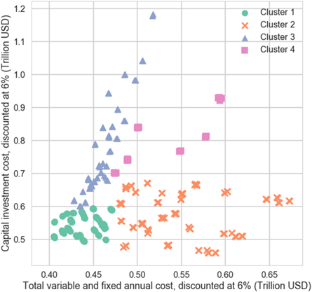
Figure 1. PRIM cluster analysis of capital cost versus variable and fixed cost for all scenarios.
Download figure:
Standard image High-resolution imageAll the clusters in figure 1 are driven by a combination of cost of capital, demand and CO2 constraint. A high cost of capital promotes technologies that have low upfront capital costs, which most often leads to investment in fossil-fuelled power plants. These tend to have a high variable cost associate with fuel purchases. However, these investment strategies are only adopted by the model, if there is no constraint on CO2 emissions. This is the case of cluster 2 (orange crosses in figure 1) in which the high cost of capital and absence, or medium level, of CO2 constraint leads to investments in fossil fuel technologies, and thus low capital costs but relatively high variable costs.
Cluster 3 (blue triangles in figure 1) is on the opposite side of the spectrum compared to Cluster 2: its outcome characteristics are only driven by a strong CO2 constraint. Cluster investments are characterised by RET deployment at a high cost (table 2).
Table 2. Results of the PRIM analysis for capital cost and variable cost.
| Determinant 1 | Determinant 2 | Determinant 3 | Coverage/Density | |
|---|---|---|---|---|
| Cluster 1: low capital cost and low variable cost | Low to medium demand (220 to 230 EJ) qp value: 10−9 | Low to medium cost of capital (3% to 6%) qp value: 10−9 | Absent or medium CO2 constraint qp value: 10−4 | 83%/83% |
| Cluster 2: low capital cost, high variable cost | High cost of capital (12%) qp value: 10−12 | Absent or medium CO2 constraint qp value: 10−7 | 65%/83% | |
| Cluster 3: high capital cost, low variable cost | CO2 constraint (strong) qp value: 10−27 | 82%/85% | ||
| Cluster 4: high capital cost and high variable cost | High demand (250 EJ) qp value: 10−12 | CO2 constraint (medium) qp value: 10−12 | Medium to high cost of capital (6% to 12%) qp value: 10−5 | 100%/100% |
Cluster 4 (pink squares) is characterised by high capital and high variable costs. These scenarios are driven by high demand levels; combined with medium to high cost of capital; in futures with a medium CO2 constraint. The high demand leads to higher costs, but this is exacerbated by the combination of a high cost of capital (which favours fossil fuel technologies) and a medium CO2 constraint (which favours renewables). The result is a trajectory in which there are high investments in fossil-fuel generation at the beginning of the period (by 2030), followed by stranded fossil fuel capacity and high renewable penetration towards the end of the period (by 2050). Note that the CO2 cap peaks in 2040.
At the opposite end of the spectrum, the first cluster (green circles) has limited capital and variable costs. It is characterized by low to medium levels of both demand and cost of capital combined with either an absence, or a medium level, of CO2 constraint (table 2).
Cost results as a percent of GDP
To better compare scenario results with past investments, we report total investment cost as percentage value of projected GDP (figure 2). Most scenarios have a total discounted system cost below 1.4% of the projected GDP associated with its respective scenario. (For context, the region spent 1.4% of GDP on energy investments before investments declined in the years 2000s (Fay et al 2017)).
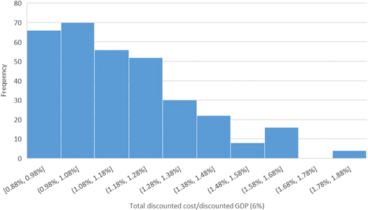
Figure 2. Total discounted cost of GDP (2013–2050) for South America for all 324 scenarios.
Download figure:
Standard image High-resolution imageA PRIM analysis is carried out on the 20% most expensive scenarios (these spend 1.34% of GDP on electricity investments). The analysis shows that they are characterized by a high demand and a medium or strong CO2-emission cap. Additionally, 60% represent a future characterised by a high cost of renewables. This combination of factors causes initial investment to focus on low capital intensity technologies (fossil fuels) which are then stranded by a switch to renewables occurring toward the end of the period. This is when the CO2 constraint becomes more stringent. While cost-optimal given the range of determinants, the strategy is expensive. This suggests that policies should be prepared to either recover the value of stranded assets, or invest in adequate retrofit schemes with e.g. carbon capture storage (CCS).
Emission based analysis of scenarios with no cap
Given that a continent wide-CO2 scheme may be difficult to impose, we focus here on scenarios without any emission caps (108 futures). Looking at determinants that lead to low/high carbon emission reveals three scenario clusters (figure 3, table 3). Cases with low-carbon emission futures are in Cluster 2 (orange crosses). They are characterised by low to medium demand and low to medium cost of capital. Conversely, the cluster with high emissions (green circles) is characterized by high demand and high cost of capital (12%). These are the futures in which fossil fuel power plants are optimal investments. Interestingly there is little impact on costs and emission levels when fuel prices change. This reflects the critical role that financial incentives (e.g. low interest loans) and demand reduction can have, highlighting that—for CO2 emissions reduction—both can be more important than the use of an emission cap.
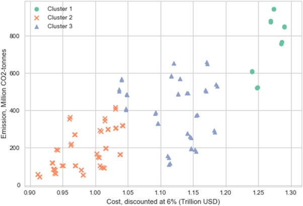
Figure 3. PRIM cluster analysis of emissions versus cost for the 108 scenarios with no CO2–cap.
Download figure:
Standard image High-resolution imageTable 3. Results of the PRIM cluster analysis for CO2-emissions.
| Determinant 1 | Determinant 2 | Coverage/Density | |
|---|---|---|---|
| Cluster 1: high emissions, high cost | High demand (251 EJ) qp value: 10−6 | High cost of capital (12%) qp value: 10−6 | 100%/100% |
| Cluster 2: low emissions, low cost | Low to medium demand (220 to 230 EJ) qp value: 10−9 | Low to medium cost of capital (3%,6%) qp value: 10−7 | 92%/100% |
| Cluster 3: medium emissions medium cost | High demand (251 EJ) qp value: 10−3 | 54%/66% |
Changes in capacity and cost for the six determinants
Demand is identified as a determinant for overall system cost, both in absolute and relative terms (percent of GDP). That is because additional electricity demand leads to additional capacity and/or additional fuel consumption. Both result in increased average total cost of electricity11 with values ranging from 123 USD/MWh in low demand cases to 154 USD/MWh in high demand futures. None of the low demand scenarios exceeds a total cost of 1.12 trillion USD, whereas the high demand scenarios consistently stay above 1.11 trillion USD. There is also a strong correlation between demand, overall system cost and emission levels.
The cost of capital is a determinant of whole system cost and CO2-emissions. The technology changes under different costs of capital have similar characteristics. High cost of capital will favour technologies with low upfront investment costs to minimize depreciation or interest during construction. These technologies include Gas, Biogas, Coal, and Photovoltaic (figure 4). A higher cost of capital will favour biogas over biomass. This is due to the seasonality of the biomass compared to the year round availability of biogas.
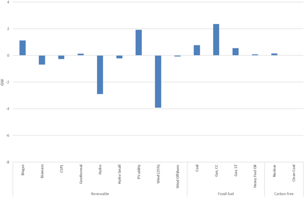
Figure 4. Average change in capacity from low cost of capital to high.
Download figure:
Standard image High-resolution imageRET learning rates—or rather the lack thereof—have a lower impact than might be expected. They are found to be the third most significant factor for explaining high total system costs, when combined with a high demand and a CO2 target. There is however a noticeable shift away from wind and PV panels in scenarios with higher RET costs (figure 5). The capital cost for PV (in 2050) varies between 422 USD/kW and 1897 USD/kW across RET learning rate futures. These are modest values when compared to hydropower, coal and nuclear per unit capacity costs, yet the latter however favoured under low RET learning rates. Nuclear has both higher per kW carbon free power output than either PV or wind. Further, the variability of wind and solar input requires intermittency contingency capacity either in the form or storage or of production capacity for wind-still or cloudy days and nights.

Figure 5. Average capacity changes of technologies from low RET cost to high.
Download figure:
Standard image High-resolution imageThe CO2-emission cap is a significant determinant for both capital and operational system costs. The 'no emission limit' scenarios never exceed 1.3 trillion USD. Conversely, the zero emissions scenarios can have costs of up to 1.7 trillion USD. Importantly, there are trajectories that can meet zero emission scenarios at a low cost (below 1 trillion USD). The common characteristics for such trajectories are low demand and a low cost of capital.
Looking at stranded assets, figure 6 illustrates fossil-fuel power plant capacity under zero emissions scenarios. These still have operating life after 2050 with a range of installed capacity of between 50–85 GW for the whole region. Similar to the PRIM analysis for capital and operational cost, demand and discount rate are main determinants of stranded asset levels in the zero emissions scenarios (table 4). Further, looking at Cluster 4 (pink squares) shows that low to medium renewable technology capital costs decrease total system cost without necessarily decreasing overall stranded asset capacity.
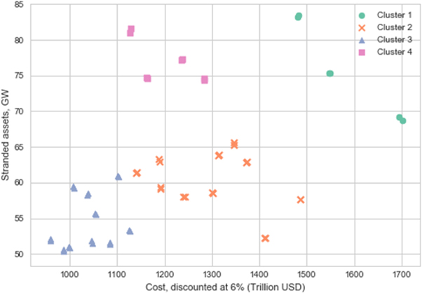
Figure 6. PRIM cluster analysis of stranded assets in zero emissions scenarios (GW) (108 scenarios).
Download figure:
Standard image High-resolution imageTable 4. Results of the PRIM analysis for stranded assets.
| Determinant 1 | Determinant 2 | Determinant 3 | Coverage/Density | |
|---|---|---|---|---|
| Cluster 1: high capacity, high cost | High demand (251 EJ) qp value: 10−6 | High cost of capital (12%) qp value: 10−6 | 100%/100% | |
| Cluster 2: low capacity medium cost | Medium to high demand (230 to 251 EJ) qp value: 10−3 | Low to medium cost of capital (3%,6%) qp value: 10−2 | 80%/66% | |
| Cluster 3: low capacity, low cost | Low to medium demand (220 to 230 EJ) qp value: 10−5 | Low to medium cost of capital (3%,6%) qp value: 10−5 | 100%/83% | |
| Cluster 4: high capacity, medium cost | High cost of capital (12%) qp value: 10−8 | Low to medium demand (220 to 230 EJ) qp value: 10−3 | Low to medium learning rates of renewable technologies qp value: 10−3 | 100%/100% |
Removing the CO2-emission limit has distinct impacts in terms of installed capacity with mixes shifting from low-carbon technologies such as Nuclear, Biogas and Wind to e.g. Gas and Coal. Some technologies prove to be competitive regardless of the CO2-emission cap: PV is also favoured in the high emissions scenarios. This implies that nuclear energy ambitions are likely to be a function of government support.
Fossil fuel price and climate change impact scenarios were not identified as significant determinants in the PRIM analysis. The first is linked the changes in fossil fuel price impacting mainly the price of oil, which is not widespread for electricity generation in South America (for details see appendix B, figure B7). Natural gas, much more widely used in the region, has a variation in price of 0.39 USD/GJ (IEA 2015). Similarly, climate change impacts across the continent are reflected by changes in hydropower capacity factor changes for South America of −0.5% from 2013–2050. Additionally, planned hydropower projects (48.8 GW) are included in the base model which and are therefore installed across all possible futures. The change of −0.5% in the capacity factor will not be a determining factor for further investments for hydropower.
Discussion
Cost of capital and fossil fuel price
Low-carbon pathways are generally correlated with perceptions of low investment risk. As results show, fossil fuel prices are not a significant driver of either whole system cost or low-carbon futures for South America and would not, at modelled levels, have enough impact to turn the system towards a low-carbon future. The cost of capital however is found to be a key determinant throughout our analyses with low cost of capital favouring more capital-intensive, often low-carbon, technologies. Higher levels of perceived risk, conversely, increase the cost of capital and hamper the introduction of these same technologies (Schmidt 2014, Iyer et al 2015b).
Both financial and political measures can be introduced to help de-risk these investments. Examples of 'financial' interventions might include subsidizing the interest rate or offering tax breaks for low-carbon technologies. Political 'interventions' could include the removal of barriers in the associated investment environment - such as streamlining the construction process (Carbon Pricing Leadership Coalition 2017).
Curbing the demand
Demand reduction has an important effect on both emissions and relative scenario costs. Contingent on them being cost effective, energy efficiency measures could decrease electricity demand without affecting major economic processes or decreasing living standards. As they would lower supply-side investment requirements, such measures would not need to mobilise higher levels of funding. By mapping the cost of energy efficiency measures under a US utility's efficiency program, Hoffman et al (2017) found the 'savings-weighted average cost' of efficiency measure to be 46 USD/MWh12 across all sectors. The residential sector cost averaged at 30 USD/MWh whereas for the non-residential sectors cost savings averaged at 53 USD/MWh. Residential sector measures included the deployment of energy efficient lighting and appliances. Non-residential sector measures were mainly prescriptive and custom rebate program based.
These results indicate that efficiency measures are cheaper to implement compared to expanding power capacity. While US and South American conditions are different, the energy efficiency costs from Hoffman et al of 46 USD/MWh compare to the cost of increasing the demand in South America which ranges from 123 USD/MWh to 154 USD/MWh. In addition to energy efficiency measures, demand-side management systems (DSM) also offers peak shaving and can thus reduce the need for peaking or backup power plants. DSM (including demand response) systems also provide opportunities to utilize the energy from intermittent capacity such as wind and solar (IRENA 2015).
These findings suggest that energy efficiency and DSM should be the focus of future refinements of the OSeMOSYS based scenario discovery approach presented in this paper.
Trade in the region
South America has significant natural resources along with large inter-connection and trade capacity. Together, these can protect the region from expensive generation options that are higher up the supply curve. Note however that this may change under cases with limited trade where countries with lower hydropower resources, unable to rely on their neighbours, may need to resort to more expensive options that drive up the cost to consumers. Further analysis may include the 'degree of inter-connectedness' as an additional scenario matrix dimension.
The CO2 cap is set to the same target over all the countries, which provides information about the implications of the CO2 cap in the region. As the countries are interconnected and have different NDC targets, analysis into the possible carbon leakages would also represent interesting future work.
CO2-emission cap can lead to higher costs
With a high cost of capital, it is optimal to keep investing in gas generation ahead of the net zero-emissions cap in 2050 after which phasing out of fossil-fuelled power leaves idle capacity which remains unused (between 50–85 GW). In order for the system to have zero emissions, the reserve margin for the zero-emission scenarios has to be supplied by low-carbon technologies. These scenarios therefore lead to additional low-carbon capacity installation. This is consistent with other work (Lecuyer and Vogt-Schilb 2014), that notes that stranded assets increase the cost of the transition, and might be politically unacceptable (Rozenberg et al 2014b). There are several ways of mitigating this issue. One would be to use the idle fossil capacity to supply the reserve margin while investing in negative emissions options including e.g. CCS of the forestry sector. Another way is to lower capital costs by offering financial incentives for stakeholders to invest today in larger renewable capacity (see for instance the chapter on Finance in (Fay et al 2015)). Appropriate concessionary finance, with low interest rates on borrowing, may be an important key to unlocking clean growth.
Conclusions
In this paper we apply a simple approach to 'discover' both scenarios of interest, and determinants of their attributes. This was undertaken on a case study of the South American electricity system, in its most detailed regional model. We find that it is easy to relate scenario attributes to their inputs for a larger ensemble of model runs that might ordinarily be attempted. The relationships and thereafter the insight gained are valuable. Two general lessons are learned. First, there is little to limit the exploration of a much larger set of inputs (we identify degree of interconnectedness as being one). Second, rather than trying to design, or understand, the role of some input 'within' a scenario, we can explore the determinants of many inputs and scenarios on an attribute of choice. This holds important insight for policy and investment outlooks that need to be formulated in anticipation of differing futures.
Results show that future investment needs in the energy sector in South America range from 1 to 2% of GDP per year depending on the scenario considered. Most of the uncertainty is driven by future demand, by the cost of capital, and by the climate mitigation constraints. In scenarios with high demand and high cost of capital—which favour fossil fuel power plants—climate mitigation constraints exacerbate tensions and significantly increase the costs.
It is however possible to completely decarbonize the electricity sector by 2050 at a low cost (below 1 trillion USD) if demand and cost of capital is low. Increases in demand could be more cost efficiently mitigated through energy efficiency measure than by increasing supply13 . Furthermore, the 'cost of capital' drives the system's structure and cost. This suggests concessionary finance products, as well as engineering-construction support, might effectively lower construction interest rates and risks. Such measures would make capital-intensive technologies like hydropower and wind more competitive. They would also prevent stranded fossil fuel capacities over the next decade should more stringent climate targets be implemented. One way of modelling concessionary financing is to have technology specific cost of capital, favouring renewable technologies.
Finally, all aspects of this work are open source14 . Together with the method applied it is hoped that adoption will be eased, transparency improved (Pfenninger et al 2018) and the tool kit needed to address increasing complexity in models more easily managed.
Acknowledgments
This research work was financed by the World Bank and Formas. Parts of the results are highlighted in (Fay et al 2017) as well as in the global infrastructure investment report 'Beyond the Gap : How Countries Can Afford the Infrastructure They Need while Protecting the Planet' (Rozenberg and Fay 2019). The initial SAMBA model on which all scenarios were built and revisions made was built by Gustavo de Moura who has been very helpful in assisting with the initial phase of the project. For the econometric modelling valuable input was provided by Gabriela Peña Balderama. For the hydrological discharge changes, the GIS-dataset was kindly provided by Ad de Roo from Joint Research Centre (JRC).
Author contribution
N M, J R, C T and O B were involved in data gathering, processing and analysis of different sections of the paper. M H and H R provided internal review and supervision. The final results were integrated by N M. N M wrote the manuscript, and all authors contributed to revising the paper.
Appendix A
Table A1. Represented technologies in SAMBA.
| Technologies represented in SAMBA | ||
|---|---|---|
| Renewable technologies | Fossil fuelled technologies | Storage options |
| Wind off-shore | Nuclear | Hydro power reservoir Brazil |
| Wind on-shore | Natural Gas Combined Cycle | Hydro power reservoir Venezuela |
| Solar Photovoltaics | Natural Gas Open Cycle | |
| Concentrated Solar Power | Pulverized Coal | |
| Clean coal (carbon capture and storage) | Oil Products | |
| Biomass Incineration | ||
| Biogas | ||
| Geothermal | ||
| Large Hydro | ||
| Small Hydro | ||
Table A2. Changes from SAMBA 2015 (Moura 2017) to SAMBA 2017.
| Main Model changes from SAMBA 2015 to SAMBA 2017 | |
|---|---|
| 1 | Guyana was added to the reference scenario. |
| 2 | Minimum generation equation is removed from the model file and replaced with a lower limit for the residual capacity with same percentage except for where there are too little resources in the country to meet the lower limit (valid for Ecuador, Hydropower Itaipu and Yacireta). |
| 3 | Reserve margin was implemented from 2020 with a linear increase to 15% by 2030. |
| 4 | Demand was updated according to new country projections based on Vector auto regression based on GDP, population, urbanization rate and electric vehicles penetration. |
| 5 | Renewable energy technologies: PV, Concentrated solar power, Wind on shore, Wind off-shore and Geothermal were updated to National Renewable Technology Laboratories (NREL). |
| 6 | Fuel cost is updated to international price from World Bank Commodities Price Forecast (June 2016) and World Energy Outlook (2015) for: Natural gas, Heavy fuel oil and Coal. Off shore Natural gas price was not updated. |
| 7 | Fuel cost for the domestic market is assume to be 5% less due to decreased logistical costs. |
| 8 | The OSeMOSYS model is updated to use the new storage equations (version 2016–08–01). |
| 9 | New output variables are added to the OSeMOSYS model file: Total Non-Discounted Cost and Total Non-Discounted Cost By Technology. |
| 10 | Paraguay electricity system is merged into one system instead of two (Itaipu and Yacireta) as the trade in the Paraguay system with a reserve margin gives skewed results (BACKSTOP) which is not realistic. |
| 11 | Transmission cost between the countries is decreased to 1USD/GJ to allow more trade between the countries. |
| 12 | Wind capacity factors are modified to a hourly shape per country to avoid wind being installed as baseload using data from Renewables Ninja for GDP coordinates with good wind potential based on wind map from dESA KTH. |
| 13 | Capacity credits for all countries were updated for the reserve margin. |
| 14 | CO2 emission cap was updated to (1) no limit (2) 50% reduction by 2050 from 2013 CO2 emissions 3) 0% emission by 2050 with peak in 2020. |
| 15 | Hydropower capacity factors is adjusted to climate change based on Representative Concentration Pathway 8.5 W m−2 for all Hydropower technologies. |
| 16 | Renewable technologies are allowed to install more per year later in the model period (2030 –>) as long as there are natural resources in the country. |
Appendix B
Appendix. Demand projection
Forecasting the electricity consumption using econometric approaches have been widely used e.g. (Mohamed and Bodger 2005, Bianco et al 2009), using economic and demographic variables as predictors. The demand projections for SAMBA are divided into three steps. First, the electricity consumption is forecasted using econometric forecasting Vector Auto-Regression (VAR) or Vector Error Correction Model (VECM). The predictors used in the analysis are GDP and population forecasts for the 10 countries (except for Guyana as data was unavailable, where respective growth rate was applied) as seen in table B1.
Table B1. Dataset for the VAR and VECM (UN DESA Population division 2015) (World Bank, WDI 2016) (IIASA 2013).
| Historical data (1971–2015) | Forecasting data 2015–2060, Shared socioeconomic pathways SSP1-SSP5 |
|---|---|
| Electricity consumption: World bank WDI Electricity consumption/capitaa UNDESA Population | GDP: OECD Env-Growtha |
| Population: UNDESA Population | POP: OECD Env-Growtha |
| GDP (current $): World Bank WDI |
aFor both population and GDP the growth rate was applied to the historical data so discrepancies between the data would not affect the transition.
Appendix. Methodology
As illustrated in figure B1, the evaluation process for the VAR and VECM follows three steps.
- 1.To avoid spurious regression analysis a unit root test is preformed to determine whether the variables are stationary or not. For the test, the Augmented Dickey-Fuller (ADF) test is used for both intercept and time trend (for results, see table B2).
- a.If all variables are stationary at first difference I(1), a Johansen co-integration test is performed. If there are co-integrated equations, then Vector error correction model (VECM) is performed (for results see table B3).
- b.For the mixed integration degrees an unrestricted VAR model is developed where the variables are differentiated if non-stationary.
- 1.For all residuals a heteroskedasity test, serial correlation test and normality test are performed to see if the residuals are white noise (for results see table B4).
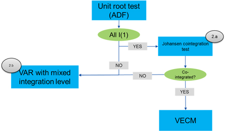
Figure B1. Evaluation process for the demand projection for GDP and Population.
Download figure:
Standard image High-resolution imageTable B2. Unit root test for all countries.
| Augmented dicker-fuller (Trend and intercept) | ||||||
|---|---|---|---|---|---|---|
| Level | First difference | Second difference | ||||
| Unit root test | Variable | p-value | p-value | p-value | Integration order | Methodology |
| Argentina | Electricity consumption | 1 | 0*** | I(1) | VAR | |
| GDP (current $) | 0.9963 | 0.0001 *** | I(1) | |||
| Population | 0 | I(0) | ||||
| Brazil | Electricity consumption | 0.9999 | 0 *** | I(1) | VAR | |
| GDP (current $) | 0.9998 | 0.0001 *** | I(1) | |||
| Population | 0.0021 *** | 0.2468 | I(0) | |||
| Bolivia | Electricity consumption | 1 | 0.026 ** | I(1) | VAR | |
| GDP (current $) | 1 | 0.034 ** | I(1) | |||
| Population | 0.03 ** | 0.2545 | I(0) | |||
| Chile | Electricity consumption | 0.999 | 0.0258 ** | I(1) | VECM | |
| GDP (current $) | 1 | 0.0041 ** | I(1) | |||
| Population | 0.9765 | 0.003 ** | I(1) | |||
| Colombia | Electricity consumption | 0.9987 | 0 ** | I(1) | VAR | |
| GDP (current $) | 1 | 0.9954 | 0 *** | I(2) | ||
| Population | 0.1195 * | 0.8743 | 0.5379 | I(0)* | ||
| Ecuador (ln) | Electricity consumption | 1 | 0.001 *** | I(1) | VECM | |
| GDP (current $) | 1 | 0.0027 *** | I(1) | |||
| Population | 0.093 * | I(1)* | ||||
| Paraguay (ln) | Electricity consumption | 0.9999 | 0.0145 ** | I(1) | VAR | |
| GDP (current $) | 0.999 | 0.0037 *** | I(1) | |||
| Population | 0.0344 ** | I(0) | ||||
| Peru | Electricity consumption | 1 | 0 *** | I(1) | VECM | |
| GDP (current $) | 1 | 0.0001 *** | I(1) | |||
| Population | 0.5809 | 0.1144 * | 0.1745 | I(1)* | ||
| Venezuela, (ln) | Electricity consumption | 0.01 *** | I(0) | VAR | ||
| GDP (current $) | 0.84 | 0.002 *** | I(1) | |||
| Population | 0.0735 | 0.0158 ** | I(1) | |||
| Uruguay, (ln) | Electricity consumption | 0.0033 ** | 0.0094 | I(1) | VAR | |
| GDP (current $) | 0.0484 ** | 0.0061 | I(1) | |||
| Population | 0.1261 * | 0.3482 | 0.0156 | I(0) | ||
***, ** 1% resp. 5% significance. * denotes variable which has been chosen with lower significance than 10%.Vector error correction model (VECM), Vector auto regression (VAR).
Table B3. Johansen integration test results.
| Johansen cointegration test | Trace test | ||||
|---|---|---|---|---|---|
| Number of cointegrated variables | Eigenvalue | Statistic | Critical value | Prob.a | |
| Chile | Nonea | 0.928 606 | 132.496 | 42.915 25 | 0 |
| At most 1 | 0.279 301 | 24.274 92 | 25.872 11 | 0.078 | |
| At most 2 | 0.232 439 | 10.846 03 | 12.517 98 | 0.0936 | |
| Ecuador | Nonea | 0.843 38 | 91.822 91 | 42.915 25 | 0 |
| At most 1 | 0.253 687 | 15.811 64 | 25.872 11 | 0.5077 | |
| At most 2 | 8.88E-02 | 3.814 606 | 12.517 98 | 0.7688 | |
| Peru | Nonea | 0.882 106 | 114.9895 | 42.915 25 | 0 |
| At most 1b | 0.438 365 | 27.3327 | 25.872 11 | 0.0327 | |
| At most 2 | 0.085 838 | 3.679 643 | 12.517 98 | 0.7878 | |
aTrace test indicates 1 cointegrating eqn(s) at the 0.05 level. bTrace test indicates 2 cointegrating eqn(s) at the 0.05 level.
Table B4. Residuals diagnostics of the auto-regression.
| Country | Heteroskedacity test (ARCH) | Histogram test | Serial correlation | Comment |
|---|---|---|---|---|
| Argentina | 0.8955 | 0.02 | 0.1634 | The residuals are not serial correlated nor heteroskedastic which is good. The residuals are though not normally distributed. |
| Brazil | 0.6785 | 0.000 001 | 0.6848 | The residuals are not serial correlated nor heteroskedastic which is good. The residuals are though not normally distributed. |
| Bolivia | 0.7533 | 0 | 0.0614 | The residuals are not serial correlated nor heteroskedastic which is good. The residuals are though not normally distributed. |
| Chile | 0.8996 | 0.71 | 0.219 | The residuals are not serial correlated nor heteroskedastic which is good, and normally distributed. |
| Ecuador | 0.5378 | 0.44 | 0.6255 | The residuals are not serial correlated nor heteroskedastic which is good, and normally distributed. |
| Paraguay | 0.4629 | 0.35 | 0.0679 | The residuals are not serial correlated nor heteroskedastic which is good, and normally distributed. |
| Peru | 0.8573 | 0.0001 | 0.3593 | The residuals are not serial correlated nor heteroskedastic which is good. The residuals are though not normally distributed. |
| Venezuela | 0.1798 | 0.17 | 0.74 | The residuals are not serial correlated nor heteroskedastic which is good, and normally distributed. |
| Uruguay | 0.777 | 0.69 | 0.1002 | The residuals are not serial correlated nor heteroskedastic which is good, and normally distributed. |
Step 2.
Urbanization rates are based on SSP1-SSP5 and connected to respectively forecasted SSP. The rates stay the same for SSP1, SSP4 and SSP5, thus the change in urbanization is accounted for only in SSP2 and SSP3 as seen in equation B.
Appendix. Equation B. Demand calculation for GDP, POP and Urbanisation rate
The delta between urban demand compared to rural demand is estimated for Bolivia in (Peña et al 2017) at 349 kWh/capita in 2035. Bolivia is a country in the region with a high urbanization rate. Its delta is assumed representative for the other South American countries. The data was extrapolated to 2060 with a difference between urban and rural consumption of 510 kWh/capita.
Step 3.
The electric vehicle (EV) electricity consumption from (Guivarch and Fisch 2016) is defined for Latin America based on the EMF-450 scenario from Assessment Report 5 (AR5) scenarios. There are 6 scenarios developed for the transport sector, which follow the narrative of the AR5 scenarios. The assumed corresponding SSPs with the transport scenarios from AR5 scenarios are illustrated in figure B2. The data were disaggregated in two steps. First, the total electricity demand was divided by the projected population for EMF-450 scenario. Second, the electricity demand per capita was multiplied by each SSP projected population per country.
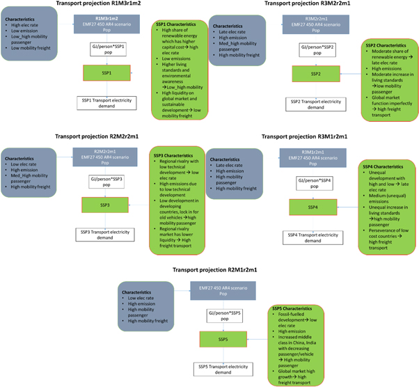
Figure B2. Connected Electric vehicle projection to each SSP.
Download figure:
Standard image High-resolution imageThe electricity demand from transportation was assumed to be an additional demand which was not included in any of the previous steps. Thus the EV demand/capita was added to the total demand.
The results did not reach satisfactory levels in the VAR/VECM analysis for Colombia. Colombia and Guyana was therefore assumed to have the average growth rate of South America for each SSP scenario. The final results for the region can are illustrated in figure B3.

Figure B3. Demand projections for SAMBA.
Download figure:
Standard image High-resolution imageAppendix. Renewable technologies learning curve
Renewable technology learning curves were based on the National Renewable Laboratories (NREL) projections (NREL 2016). The RET technologies with learning potential considered in the analysis are: On-shore Wind, Offshore Wind, Solar Utility PV, CSP and Geothermal. Two parameters are considered for the learning curves: Efficiency and cost. As shown in figure B4 the highest capital cost reductions are for CSP, Off-shore Wind and PV.

Figure B4. Renewable technologies capital cost.
Download figure:
Standard image High-resolution imageRegarding capacity factors, seen in figure B5, learning curves are related to wind power while other technologies are expected to stay the same throughout the modelling period. (Therein efficiency and cost improvements are assumed to fully account for the learning).

Figure B5. Renewable technologies capacity factors.
Download figure:
Standard image High-resolution imageAppendix. Discount rate
The discount rate was set to 3%, 6% and 12% to represent a spread of plausible pathways. For all power plant technologies, the discount rate was similarly used to represent interest rate during construction (IDC)—thus capturing the cost of borrowing capital and not simply the overnight cost. The modelled costs for the three discount rates are illustrated for 2013 and 2050 in table B5 (renewable technologies are based on medium cost). For the renewable technologies the capital cost is dynamic, meaning that depending on the combination of discount rate and renewable technology (with its respective learning) the capital cost varies with both the discount rate and the technology cost profile.
Table B5. Capital cost with IDC for all technologies, (Renewable technologies medium cost).
| 3% | 6% | 12% | ||||
| Technology | 2013 | 2050 | 2013 | 2050 | 2013 | 2050 |
| Biogas | 2026 | 2026 | 2272 | 2272 | 2832 | 2832 |
| Biomass | 1576 | 1576 | 1767 | 1767 | 2203 | 2203 |
| Clean Coal | 5402 | 3801 | 6060 | 4263 | 7553 | 5314 |
| Coal | 2589 | 1932 | 2904 | 2167 | 3619 | 2700 |
| CSP | 8769 | 3861 | 9558 | 4209 | 11 274 | 4965 |
| Distribution | 1422 | 1422 | 1463 | 1463 | 1546 | 1546 |
| Gas, CC | 1093 | 1093 | 1191 | 1191 | 1405 | 1405 |
| Gas, ST | 530 | 530 | 562 | 562 | 627 | 627 |
| Geothermal | 5140 | 5140 | 5766 | 5766 | 7186 | 7186 |
| Heavy Fuel Oil | 1273 | 1273 | 1348 | 1348 | 1505 | 1505 |
| Hydro | 2048 | 2048 | 2359 | 2359 | 3095 | 3095 |
| Hydro Small | 3183 | 3183 | 3371 | 3371 | 3763 | 3763 |
| Nuclear | 5680 | 5004 | 6557 | 5776 | 8635 | 7607 |
| PV utility | 2037 | 857 | 2096 | 882 | 2215 | 932 |
| T&D | 608 | 608 | 626 | 626 | 661 | 661 |
| Wind (25%) | 1994 | 1929 | 2173 | 2102 | 2563 | 2480 |
| Wind Offshore | 5891 | 4029 | 6421 | 4391 | 7575 | 5180 |
The life span, fixed and variable cost of each technology was obtained from the Energy Technology Systems Analysis Program (ETSAP) Technology Brief reports (IEA ETSAP 2010a, 2010b, 2010c, 2010d, 2010e, IEA ETSAP 2010a, 2010b, 2010c, 2010d, 2010e, IEA ETSAP 2010a, 2010b, 2010c, 2010d, 2010e, IEA ETSAP 2010a, 2010b, 2010c, 2010d, 2010e, IEA ETSAP 2010a, 2010b, 2010c, 2010d, 2010e, IEA ETSAP 2013a, 2013b, IEA ETSAP 2013a, 2013b, IEA ETSAP 2014). For fossil fuel technologies, the thermal efficiency and its corresponding future improvements was obtained from the Energy Technologies Perspectives report (IEA ETP 2012, IEA ETP 2014, IEA ETP 2015).
Appendix. CO2-emission cap
The CO2-emission cap was set to three levers:
- (1)No limit
- (2)50% reduction of 2013 emissions by 2050, with a peak in 2040.
- (3)0% emissions by 2050 with a peak in 2020.
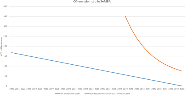
Figure B6. CO2-emissions cap.
Download figure:
Standard image High-resolution imageThe capacity changes with changes (as a function of demand, but also) in technology investment—in particular as variable renewable energies are added. This reflects the power system reliability needs—and the requirement to maintain an invoke-able reserve margin. The reserve margin is the difference between the effective installed capacity and the system peak load, expressed in percentage value. A functional power system usually operates with 15%–18% reserve margin (Rochlin 2004). These vary as a function of system specifics, reliability requirements, risk perception and other factors. For SAMBA, a 15% reserve margin was set for all countries. To account for variability, and yet maintain a reserve margin, 'capacity credits' are assigned. These represent the amount of capacity for which can be accounted for the reserve margin. For the SAMBA model the chosen capacity credits are shown in table B6 where solar and wind power would have a lower capacity credit as the timing of the peak demand might not coincide with the availability of solar and wind.
Table B6. Capacity credits for all technologies in SAMBA.
| Technology | Capacity credit |
|---|---|
| Biogas | 100% |
| Gas, CC | 100% |
| Geothermal | 100% |
| Heavy Fuel Oil | 100% |
| Hydro | 100% |
| Nuclear | 100% |
| Gas, ST | 100% |
| Wind Offshore | 5% |
| Wind (25%) | 5% |
| PV utility | 5% |
| CSP1 | 30% |
| Clean Coal | 100% |
| Coal | 100% |
| Geothermal | 100% |
| Biomass | 66% |
Because the energy system in the 0% emissions scenario has no carbon emissions, the reserve margin contributions from fossil fuelled technologies are from 2040 gradually phased out. By 2050 only carbon free technologies are allowed to satisfy the capacity reserve constraint. With their associated capacity credit, total investment numbers increase.
Appendix. Fossil fuels price development
The fossil fuel price development is based on two reports: World Bank Commodities Price Forecast (constant US dollars) July 2016 and World Energy Outlook (2015) (World Bank 2016, July) (IEA 2017). For the years 2013–2025 all scenarios are based on the same forecasted price from World Bank Commodities Price Forecast (figure B7). From 2025–2040 the two projected scenarios: Current policies scenario (high) and Low oil price scenario (low) is applied. From 2040 and onwards the Compound Annual Growth Rate (CAGR) from 2013–2040 is applied.
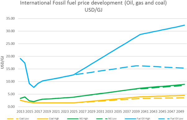
Figure B7. Fossil fuel price development.
Download figure:
Standard image High-resolution imageMany of the South American countries have large reserves of fossil fuels and the domestic price of fuels are assumed to be 5% cheaper than the international price due to reduced costs for logistics. Trade between the interlinked countries such as Argentina and Bolivia the international price is assumed for the consuming country.
Appendix. Climate change affecting hydro power
The climate change scenario has two levers: one with a static future climate and the other with a climatic change following the Representative Concentration Pathway (RCP) 8.5. The RCP 8.5 is the scenario with the highest emissions and temperature changes for AR5 (IPCC 2007, 19–21 September). The data which was used were from two data sets:
- (1)Discharge projection (Alfieri et al 2017) 2006–2057. The monthly average discharge was identified for locations with existing hydro power plants (Geofabrik 2016) (as seen in figure B8). This was identified based on changes in the geographically closest location. Discharge data was aggregated to the level at which generation data is available.
- (1)Monthly generation data for all hydro technologies are considered in SAMBA. For power plants in Brazil and Venezuela with hydro storage, the Affluent Natural Energy (ANE) was modelled instead of generation as this is more closely connected to the discharge compared to the generation collected from the national databases: (CONELEC 2010, Goberno de Bolivariano de Venezuela 2012, Autoridad de Fiscalización y Control Social de Electricidad 2013, COES 2013, ADME 2013, Comisión Nacional de Energía Atómica 2013, ONS 2013, SIEL 2014, CNE 2015).
Appendix. Exceptions
In the case of Guyana and Tele Pires, generation data was not available and were instead based on discharge change from 2013 (average of 2006–2013) to 2050 (average 2045–2055). Bel Monte Dam, Paraguay Large hydro, Tapajos, Madeira did not have available discharge data nor generation data and the closest regional change was assumed for these.
Appendix. Methodology
To be able to use the discharge as a predictor, a vector auto regression (VAR) with seasonal adjustment with dummy variables was applied. The following steps for the VAR for each hydro technology in SAMBA were executed.
- 1.Unit root test (Augmented Dicker Fuller) to assess if the process (both generation and discharge) is stationary.
- 2.Unrestricted VAR with generation as dependent variable, discharge as endogenous and dummy variables as exogenous.
- 3.Lag-length criteria is assessed from Akaike Information Criterion (AIC) and Schwarz Information Criterion (SC) to find the optimal lag length.
- 4.Evaluation of the quality of the forecast is based on R-squared, Durbin-Watson, AIC, Root Mean Square Error (RMSE), Covariance Proportion and Thiel Inequality coefficient.
- 5.The process is reiterated from step 2 to find the best fit with different seasonal division (6 months, 12 months and no season).
To keep the model from having any changes from the 'no climate change' scenario in the starting years the percentage change from the VAR was applied to existing capacity factors to keep consistency between scenarios. All percentage changes were calculated on a monthly basis to capture the seasonal changes of generation with climate change.
The results are shown in figure B9 for both the discharge changes (average of 2006–2013 to average of 2045–2055) and forecasted generation changes (2013 to average of 2045–2055). In general, the discharge changes are higher than the generation changes.
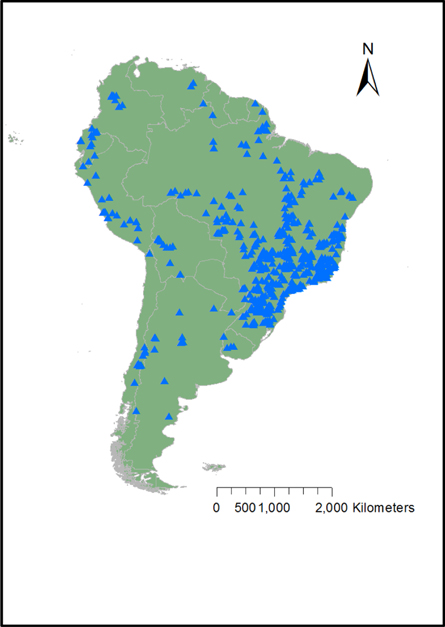
Figure B8. Modelled hydro power plants in South America developed in ArcGIS.
Download figure:
Standard image High-resolution image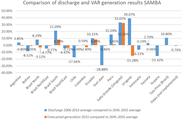
Figure B9. Changes in the electricity generation compared to the discharge.
Download figure:
Standard image High-resolution imageA study by (Schaeffer et al 2008) analysed the impact of climate change in hydrology for Brazil. Schaeffer et al based their analysis on the Special Report on Emissions Scenarios (SRES) A2 scenario, which in Assessment Report 4 (AR4) was the high emissions scenario. They found a hydrology generation impact of −1% for Brazil for the period 2071–2100. The results from this study found an overall generation impact for Brazil of −1.5% for the RCP 8.5 for the period 2045–2055. Comparing the RCP 8.5 to SRES the scenario it is comparable to the A1F1 scenario which has higher emissions than A2 (IPCC 2000, SEI 2016). The higher impact in this study can be explained by the difference in scenario projections.
Footnotes
- 6
All data is available on zenodo.org: https://doi.org/10.5281/zenodo.2238771.
- 7
The lever represents the different levels that the input parameters are set to.
- 8
Note that in this formulation, 'variable cost' is assumed to include both variable maintenance and fuel costs.
- 9
- 10
This is a social discount rate, to be distinguished from the 'cost of capital' used as an input parameter to the model results.
- 11
 where N is the lifetime in years (here assumed the modeling period, 38 yeras)
 - 12 where N is the lifetime of measure in years.
- 13
As such, further analysis on efficiency measures would be the next step to see the impact in the electricity system. Furthermore, as Welsch et al (2012) developed a module for Smart Grid modelling in OSeMOSYS, peak shaving of demand in the South American system would also be an important future task.
- 14
