
Abstract
Artificial neural networks can be an important tool to improve the search for admissible string compactifications and characterize them. In this paper we construct the heterotic orbiencoder, a general deep autoencoder to study heterotic orbifold models arising from various Abelian orbifold geometries. Our neural network can be easily trained to successfully encode the large parameter space of many orbifold geometries simultaneously, independently of the statistical dissimilarities of their training features. In particular, we show that our autoencoder is capable of compressing with good accuracy the large parameter space of two promising orbifold geometries in just three parameters. Further, most orbifold models with phenomenologically appealing features appear in bounded regions of this small space. Our results hint towards a possible simplification of the classification of (promising) heterotic orbifold models.
Export citation and abstract BibTeX RIS

Original content from this work may be used under the terms of the Creative Commons Attribution 4.0 licence. Any further distribution of this work must maintain attribution to the author(s) and the title of the work, journal citation and DOI.
1. Introduction
Compactifying the six extra dimensions of any of the string theories yields a huge number of four-dimensional (4D) models. Recent scans include compactifications based on intersecting D-branes [1–3], fermionic constructions [4–6], orientifolds of Gepner models [7, 8], Calabi-Yau manifolds [9–13] and supersymmetric [14–19] and non-supersymmetric [20, 21] heterotic orbifolds [22, 23]. Many of those constructions include three generations 3 of the standard model (SM), its minimal supersymmetric extension (MSSM) or their completions in grand unified theories (GUT). However, most models are not of this kind, i.e. they display features that are not compatible with observations.
The properties of the resulting 4D theories depend on the choice of the geometry of the compact space, which is characterized by some selectable parameters. Their quantity and admissible values are determined by the type of string compactification and strict consistency constraints, such as modular invariance and tadpole cancelation. The parameters and their possible values build enormous convoluted multidimensional spaces. Hence, the task of exploring all points in such parameter spaces yielding admissible models and, then, identifying among them the best candidates to describe nature becomes insurmountable or, in the best of cases, extremely challenging. Despite being time-consuming, random searches have shown certain efficacy [25–30], but we may profit from a more ingenious approach.
The latest developments of numerical methods and, specifically, of machine learning (ML) techniques for information processing along with the accessibility to faster computational hardware, has favored the applications of ML in various fields, including string phenomenology [31]. Basic numeric applications in this endeavor, such as genetic algorithms [30, 32–34], have led to more complex ML string-phenomenology setups based on decision trees [19, 35, 36], deep neural networks [37–41], support vector machines [42, 43], reinforcement learning [44–46], autoencoders [47–49], and several others [50–52].
In particular, autoencoders [53] are artificial neural networks (NN) frequently used to furnish a compressed representation of some multidimensional input data. By using them to reduce the dimensionality of their parameter spaces, they might become instrumental in the classification of string models and the identification of the most phenomenologically suitable ones.
We focus here on (Abelian toroidal) orbifold compactifications of the E8×E8 heterotic string in the bosonic formulation. In their simplest form, they correspond to assuming that the compact space adopts the structure given by the quotient  , where S denotes any of the Abelian space groups classified in [54]. Once S and thereby the orbifold geometry is chosen, modular invariance demands the orbifold to be embedded in the gauge degrees of freedom of E8×E8, which can be done via eight 16-dimensional (16D) rational vectors known as shifts and Wilson lines. These 128 rational parameters are then subject to additional modular invariance conditions [55], which ensure anomaly freedom of the resulting 4D effective theory. The exploration of this 128-dimensional parameter space has been automatized in the orbifolder [56]. However, it is known that not all models can be found with this software [19]. In [47] it has been shown for one particular S that an autoencoder may pack with acceptable accuracy the properties of an orbifold in a two-dimensional latent space.
One of our goals here is to extend the results of [47], to achieve a tool capable of analyzing various space groups at the same time, aiming at a general classification of all orbifolds in a simplified latent space. This poses a challenge as models arising from different orbifold geometries exhibit very different patterns in their parameter spaces. Additionally, our tool should achieve a better accuracy than previous efforts and yield a better understanding of how promising compactifications are accommodated in the latent space. With this aim, we design a (fully connected, symmetric) deep autoencoder, which we call heterotic orbiencoder, that can receive multiple orbifold geometries and encode their information in a tridimensional (3D) latent space.
Our work is organized as follows. After a noncomprehensive review on heterotic orbifolds in section 2, we devote our section 3 to exploring a variety of architectures and function configurations (combinations of optimizer, activation and loss functions) in order to identify the optimal structure of our deep autoencoder. These findings allow us develop the heterotic orbiencoder, whose properties and commands are described in section 4. We exemplify its power by applying it on two phenomenologically appealing orbifold geometries ( –I (1,1) [57, 58] and
  –I (1,1) [59–61]) in section 5. Finally, we discuss our main observations in section 6. In our appendix we discuss some challenges we face to optimize the speed and accuracy of the autoencoder while avoiding overfitting.
2. Features of heterotic orbifolds
In order to fix our notation, let us introduce some basics on heterotic orbifold compactifications. (For more detailed discussions, see e.g. [62–65] or [18]). The space group S of a six-dimensional (6D) orbifold  leading to
  supersymmetric effective field theories at low energies can be specified by up to two generators, ϑ, ω, of the orbifold rotational subgroup, and six basis vectors eα
, α = 1,...,6, of the lattice of a
supersymmetric effective field theories at low energies can be specified by up to two generators, ϑ, ω, of the orbifold rotational subgroup, and six basis vectors eα
, α = 1,...,6, of the lattice of a  torus. An arbitrary element of S can be written as (ϑk
ωℓ
, mα
eα
) ∈ S, where 0 ≤ k < N and 0 ≤ ℓ < M,
torus. An arbitrary element of S can be written as (ϑk
ωℓ
, mα
eα
) ∈ S, where 0 ≤ k < N and 0 ≤ ℓ < M,  , such that N and M denote the orders of ϑ and ω, respectively. Further,
  only in the absence of roto-translations. It is convenient to identify the conjugacy classes of S, such that we can build a set of inequivalent space-group elements by choosing one representative from each conjugacy class.
Orbifolds have curvature singularities also known as fixed points, since they are left invariant under space group elements. Each singularity can be associated with a conjugacy class of S exhibiting nontrivial rotational action. This implies that the number of fixed points nfp depends on S, i.e. nfp = nfp(S). In order to better identify the fixed points, it is customary to split the conjugacy-class representatives into sectors labeled by the pairs (k, ℓ). A fixed point  is said to belong to the (k, ℓ) sector if there exists a conjugacy-class representative (ϑk
ωℓ
, mα
eα
) ∈ S, such that
is said to belong to the (k, ℓ) sector if there exists a conjugacy-class representative (ϑk
ωℓ
, mα
eα
) ∈ S, such that

The next building block to obtain a heterotic orbifold is the embedding of S into the 16D gauge degrees of freedom associated with E8×E8. Both the six toroidal shifts eα and the two rotational generators of S can be embedded as 16D rational gauge shift vectors. In our conventions, the gauge embedding is given by

In this embedding the vectors VA , A = 1,...,8, encode the orbifold action on the E8×E8 space as shifts in the gauge momenta. Vα are frequently called Wilson lines.
The gauge shift vectors VA must comply with a number of consistency conditions. For example, since V7 (V8) is a gauge embedding of the rotation ϑ (ω) of order N (M), then it must fulfill that NV7 (MV8) be in the root lattice of E8×E8. Hence, N and M are also known as the orders of V7 and V8, respectively. The relations among the various eα due to the actions of ϑ and ω on them, are translated as relations among the different VA , A = α = 1,...,6, that must be fulfilled, and also establish the order NA of these shift vectors. Additionally, these shift vectors must satisfy certain modular invariance conditions [55].
For each choice of S, there is a large (and unknown) number of inequivalent gauge embeddings VA that fulfill all consistency conditions, and lead to admissible 4D effective field theories. This vast set of effective theories can be regarded as the landscape of heterotic orbifold models. These models exhibit various gauge groups G4D ⊂ E8 × E8 of rank 16 and (massless and massive) matter fields building representations under G4D. One can focus only on the massless states because the fundamental scale of these constructions is the string scale, which is close to the Planck scale and hence decoupled from observable physics.
The massless matter spectrum is given by the closed strings that are invariant under the orbifold. They can be split into i) strings that are closed (and massless) prior to the orbifold action, known as untwisted strings, and ii) strings that close only due to the action of the orbifold, called twisted strings. In fact, the representatives of the conjugacy classes of S indicate how strings transform at the fixed points and, thus, are used to establish the boundary conditions of the strings to close. In this scheme, untwisted strings are associated with the (k, ℓ) = (0, 0) sector, as neither ϑ nor ω twists the strings to close in this case. Twisted strings arise from the (k, ℓ) ≠ (0, 0) twisted sectors. We focus here on untwisted strings because they yield the gauge group, which is considered in this work to be the key property of the model. 4
Untwisted matter states carry the gauge momenta p associated with the original E8×E8 gauge bosons of the heterotic string in 10D that are left invariant under the gauge embedding of the orbifold. The unbroken gauge group G4D can be obtained from requesting that the momenta p be invariant under the gauge shifts VA , which amounts to demanding that

where, for future convenience, we have separated the two E8 components, such that each p(a), a = 1,2, and  , A = 1,...,8, are elements of the eight-dimensional (8D) root lattice of E8. The E8 momenta can be written as

where the power in the entries denotes repetition, and the underscore stands for all possible permutations.
The subset I0 of the momenta (4) satisfying equations (3) builds G4D, and clearly depends on the gauge embedding vectors VA
. It will be convenient to define the subgroups  , such that
  , which are built by the invariant E8 simple roots in the subsets

Note that the same  can be generated for different (although equivalent) sets
  . This is related to the symmetries of the E8 root lattice, which include E8 Weyl rotations and lattice translations, among other transformations, see e.g. [66]. Modding out these symmetries is not feasible at the moment. However, observe that the number of invariant roots
  must be an invariant under all symmetry transformations, and can hence be used as a characteristic feature of a heterotic orbifold model.
Interestingly, at the fixed points of the twisted sectors, the closed strings related with the gauge bosons do not perceive the whole action of the orbifold, but only its local action. This is encoded in the conjugacy-class representative (ϑk ωℓ , mα eα ) ∈ S that defines each fixed point. By using equation (2), we see that the shift vector Vlocal associated with the localized action of the orbifold at such fixed point is given by

Hence, the local gauge symmetry group Glocal,n realized at the nth singularity is built by the momenta in the sets

As for the gauge group G4D associated with the untwisted sector, the cardinalities  are invariant properties of the local gauge group Glocal,n
.
are invariant properties of the local gauge group Glocal,n
.
3. Optimizing an autoencoder for heterotic orbifolds
3.1. Orbifold datasets
Considering the eight 16D shift vectors VA
that define them, heterotic orbifold models with a given space group S exhibit 128 defining parameters. However, as mentioned before, there are highly nontrivial symmetries relating different gauge embeddings that may reduce the number of truly free parameters. Noting that the symmetry invariants  encode information about the shift vectors, one might entertain the possibility to replace the original parameters by a set of cardinalities
  , which has shown to be a reasonable strategy [47].
Our purpose here is to design an autoencoder capable of analyzing models of various orbifold geometries at once. The challenge here arises from the fact that each orbifold geometry has very different properties. This implies that the defining parameters associated with each S exhibit e.g. different values and statistical characteristics, see our auxiliary material for two sample orbifold geometries [67]. We must find a method to deal with the various geometries simultaneously. For instance, since in general the total number of fixed points nfp(S) depends on S, we must restrict the selection of fixed points to a subset of size sfp, such that sfp ≤ nfp(S) and is equal for all considered space groups. In addition, we must consider a numerical label L for the space group associated with each model and, in order to capture more features about the 4D spectrum, we shall include the number of U(1) gauge factors NU(1). Therefore, we choose as characteristic features of a model the subsets

Thus, in this scenario, the number of considered features is 2sfp + 4.
There is some arbitrariness on the choice of sfp that we can use to our advantage. It is clear that the larger sfp is, the better X captures the properties of the orbifold. This is because each chosen fixed point can contain information about a single shift vector VA
and we need information about all of them. However, sfp cannot be too large because there are some space groups S that admit only a small number of fixed points. Further, taking the maximal number of fixed points of a given geometry is not necessary in general because the definition (6) of the local gauge embedding implies that there are Vlocal,n
at different singularities that can lead to the same values  . Moreover, we must also take into account that the computation time grows with the dimensionality of X. So, we find it convenient to consider sfp of order 10, and choose the fixed points from the (first) twisted sectors (k, ℓ) = (1, 0) and (0, 1) in addition to some others from higher twisted sectors, in order to capture at various (preferably geometrically inequivalent) singularities as much information provided by all shift vectors VA
as possible. Note that choosing sfp of order 10 exhausts the information coming from all eight VA
unless we incorrectly take only geometrically equivalent fixed points.
. Moreover, we must also take into account that the computation time grows with the dimensionality of X. So, we find it convenient to consider sfp of order 10, and choose the fixed points from the (first) twisted sectors (k, ℓ) = (1, 0) and (0, 1) in addition to some others from higher twisted sectors, in order to capture at various (preferably geometrically inequivalent) singularities as much information provided by all shift vectors VA
as possible. Note that choosing sfp of order 10 exhausts the information coming from all eight VA
unless we incorrectly take only geometrically equivalent fixed points.
Once the feature vector X to be used on different orbifold geometries is defined, we must build the datasets that will allow us to train the autoencoder. With this goal, one must first generate a large number (a few hundred thousands) of inequivalent admissible orbifold models with one or more space groups by using the dedicated automatized tool orbifolder [56]. This generates the 'raw data' containing a large number of sets of gauge shift embeddings {VA
}. In a second step, we run our Makedataset code [68] (detailed in section 4.1) that translates these vectors into the sets of gauge momenta  defined in equations (5) and (7) and the resulting gauge group in 4D, and then computes the invariant feature vectors X.
Due to the differences among the various orbifold geometries, the process previously described will, in general, generate very different sets of data for different geometries. This is not surprising since the process leading to the cardinalities Na n involves information that is particular to the geometry, namely the centralizers and the orbifold twisted sectors. Putting all these elements together means that dealing with more than one geometry is not just a matter of extending the data to some extra elements of a given set, it is a whole new extension to study a different problem. Including more than one geometry gives a more generic perspective of the 4D models arising and, possibly, independent of the geometry. This allows us to explore the heterotic landscape in a somewhat more general perspective.
3.2. Autoencoder configurations
A deep autoencoder is a feedforward NN, mainly used to dimensionally reduce or compress some complex high dimensional data. It is built by two components: the encoder and the decoder. The purpose of the encoder is to identify and reduce the redundancies (and noise) of input data defined by a large number of parameters, lowering step-wise in various (hidden) layers the dimensionality of the parameter space. If the encoder is deep enough, i.e. if it has a large number of layers, and the data is adequate, its capability to encode the input data into a small number of parameters tends to improve. The last layer of the encoder is known as the (central) latent layer or latent-space representation, and it contains a 'compressed code' of the input data, represented in a small number of parameters. The decoder operates inversely to the encoder, reconstructing the data from the latent layer back to its original higher dimensional form. 5 One can define the accuracy of an autoencoder as the level of likeness between the output resulting from the decoder and the corresponding original information in the input layer.
Given some input data, one must choose hyperparameters that maximize the accuracy of the algorithm. The properties that describe an autoencoder configuration are:
- Topology: overall structure that defines the way the neurons of the NN are connected among different layers. The topology can be symmetric or asymmetric with respect to the latent or bottleneck layer, fully or partly connected, and can include convolutional layers or other types of substructures. We avoid convolutional or other complex layers for simplicity. 6
- Architecture: number of layers and number of neurons per layer (layer size). In the case of an autoencoder, it includes the sizes of all hidden layers of the encoder and decoder, the input and output layers, as well as the size of the latent layer.
- Initial weight distribution: the values of the trainable parameters or weights that characterize the neurons must be initialized at random values using a method that may be useful to arrive at the best accuracy; it is customary to take a Gaussian or uniform distribution, but other options (such as Xavier or He initializations [69–73]) are possible.
- Activation function: together with a bias, it defines the output of a neuron given some input information; it adds some non-linearity to the learning process in order to improve it. Some examples that we shall use in this work include Leaky-ReLU, Softplus, ELU, CELU, ReLU, SELU, Hardtanh, Softmax and LogSigmoid (see e.g. [74–78] for details of activation functions). In principle, every layer can have a different activation function, but we apply, as usual, homogeneously the same activation function to all layers for simplicity. Despite the expectation of a poor performance of Hardtanh, Softmax and LogSigmoid, as will be confirmed, they can be used here as a basis for comparison.
- Loss function: evaluation during the training stage that determines the magnitude of the inaccuracy that the NN has achieved before updating the weights of the network. Motivated by the encouraging results of [47], where the L2 loss function (equivalent to MSE) provides a good accuracy, we decide to test various loss functions besides the most natural choice of Cross Entropy (CE). Some examples of loss functions used in this paper are CE, SmoothL1, MSE, Huber, BCEWL, L1 and Hinge Embedding (see e.g. [79, 80] for details).
- Optimizer: optimization algorithm used to minimize the loss; some examples applied in this work are Adam, AdamW, Adamax, RMSProp, Adagrad, Adadelta, SGD and ASGD (see e.g.[81–84] for details on these functions).
- Number of epochs: number of times that the algorithm is run to improve the learning skills of the algorithm, trying to minimize the error.
- Batch size: for each epoch, it is the number of samples in which the training input data is split in order to have several training subsets. Typically, large batch sizes lead to better statistical characterizations; however, although commonly varied only to adapt it to the availability of memory, we shall see that the choice of batch size can also help to improve the accuracy of the model.
- Shuffling: to optimize the learning process, whether or not the elements contained in each batch per epoch are randomly shuffled.
- Dropout: if applied, it defines the number of dropout layers and the fraction of neurons that are randomly dropped out; this is typically used with the goal of reducing overfitting.
The choice of the best configuration can be either 'handcrafted' by some educated guess or achieved by a systematic study of the properties that define the autoencoder. We mix both methods: we vary systematically three of the configuration parameters (activation and loss functions, and the optimizer) while fixing all others. In detail, based on the results of [47], we first fix the topology to be feedforward fully connected and symmetric with respect to the latent layer, the initial weight distribution to be Gaussian, and we apply shuffling of the data in each epoch.
To fix the architecture, we adapt the feature vectors X so that they can be readily handled by the autoencoder. Since the selected features are all categorical (they admit a limited set of values), it is convenient to perform a one-hot encoding (OHE). To minimize the use of resources as well as arrive at good results, we take sfp = 8, leading to 18 features which accept various different sets of values ![${N}_{n}^{(a)}\in [0,240]$](https://content.cld.iop.org/journals/2399-6528/8/2/025003/revision2/jpcoad246fieqn21.gif) . In addition, the number of U(1) gauge symmetries in 4D is constrained by 0 ≤ NU(1) ≤ 16, and L is limited by the number of orbifold geometries that one incorporates in the autoencoder. Each feature Xi
is then mapped to a subvector XOHE,i
of (different) dimensionality γi
. The resulting full one-hot encoded feature vector XOHE has dimensionality
. In addition, the number of U(1) gauge symmetries in 4D is constrained by 0 ≤ NU(1) ≤ 16, and L is limited by the number of orbifold geometries that one incorporates in the autoencoder. Each feature Xi
is then mapped to a subvector XOHE,i
of (different) dimensionality γi
. The resulting full one-hot encoded feature vector XOHE has dimensionality  . This is the size of the input and output layers. We shall aim at arriving at a three-dimensional latent layer, in order to better capture the information from various orbifold geometries. We shall include 7 or 9 hidden layers, aiming at a NN deep enough to provide admissible results.
Other configuration parameters are defined in various tests, as we now describe.
3.2.1. Testing configurations
In order to arrive at the best configuration, we have used orbifold models based on two phenomenologically promising and distinct orbifold space groups, which are known as  –I (1,1) and
  –I (1,1) in the notation of [54]. For simplicity, we label them as
  and
and  , respectively. The features and phenomenology of
  orbifold compactifications have been studied in detail in [58, 85], while many interesting properties of
  models have been presented in [59–61, 86–89]. It is known that these space groups correspond to two of the most fertile
  orbifold geometries, as they yield large sets of MSSM-like models [17–19]. We emphasize that, even though our method is trained here for these geometries, it can be generalized to any choice of geometries. While implementing our method for larger sets, one must consider that the larger the set of geometries and models is, the more computational resources are required.
With the help of the orbifolder [56], we have built a database of nearly 270,000 inequivalent, anomaly-free models from each chosen geometry, with several different gauge groups G4D. The total of 540,000 models is randomly split into a 66.7% for the training set and a 33.3% for the validation set.
In this case, we have considered sfp = 8 fixed points per geometry, 7 which means that the feature vectors X of equation (8) are 20-dimensional. Analyzing the total of our models, the OHE enhances the feature vectors to 810-dimensional one-hot encoded vectors XOHE. This represents the input layer.
After some quick tests with various libraries, we found optimal the use of PyTorch [90] and some Pandas [91] and Scikit-learn [92] functions, as they are simple and economic in notation and as effective as other options.
Now we are ready to implement and test our proposal. Since we wish to test for several activation, loss and optimizer functions, we define a basic or 'vanilla' configuration, which is given in table 1. As anticipated, we use seven hidden layers, including the 3D latent layer. The dimensions of the layers of our symmetric NN are 810, 200, 26, 13, 3, 13, 26, 200, 810. We run the training stage for 1,000 epochs, with no assumption about overfitting or other undesirable properties that we want to identify in this phase.
Table 1. Parameters of our 'vanilla' configuration. While others are fixed, we vary the parameters with the label 'default value', one at a time, in order to arrive at the best autoencoder configuration. E.g. we test different optimizers while taking the default values specified here for the activation and loss functions.
| Configuration parameters | Chosen values |
|---|---|
| Topology: | Fully connected and symmetric |
| Architecture: | 810, 200, 26, 13, 3, 13, 26, 200, 810 |
| Initial weight distribution: | Gaussian |
| Activation function: | SELU (default value) |
| Loss function: | MSE (default value) |
| Optimizer: | Adam (default value) |
| Number of epochs: | 1, 000 |
| Batch size: | 25 |
| Shuffling: | True |
| Dropout: | False |
We test the different functions of our setup as follows: we choose the one function in the vanilla configuration that we want to test and leave the other two fixed with the 'default values' given in table 1; then, we vary systematically the chosen function through the options listed in section 3.2, training the NN during 1,000 epochs for each resulting configuration. We tested various batch sizes ranging from 23 to 27, which are within the capabilities of any small or large computer, and observed that varying the batch size also allowed us to arrive at a better accuracy. Finally, we arrived at a batch size of 25 = 32 to minimize the hardware demands while aiming at good results. 8 The default values are considered taking into account their good performance in NN for similar purposes and their reduced computing time. In order to evaluate the performance of each configuration, we examine the NN accuracy and loss.
While assessing the results, we realized that the typical definition of the loss function, which compares the full predicted and input feature vectors, exhibits some weakness because of the large number of zeroes appearing in the one-hot encoded vectors that are compared. We improve this situation by demanding that the loss function compare the input and output one-hot encoded vectors by feature. In detail, we implement the redefinition of the loss

where i runs over all features, j over all elements of a batch, and k over all batches in the training set. As usual, XOHE denotes the input one-hot encoded feature vector, and  the prediction of the autoencoder. The chunk
  associated with the ith feature of the jth element of the kth batch has dimensionality γi
, which is the number of values that the ith categorical feature admits. The loss function F( · , · ) is chosen here to be one of our testing set: Cross Entropy (CE), SmoothL1, MSE, Huber, BCEWL, L1 and Hinge Embedding.
associated with the ith feature of the jth element of the kth batch has dimensionality γi
, which is the number of values that the ith categorical feature admits. The loss function F( · , · ) is chosen here to be one of our testing set: Cross Entropy (CE), SmoothL1, MSE, Huber, BCEWL, L1 and Hinge Embedding.
Our results at this stage are presented in figures 1–3. In figure 1 we show a comparison of the evolution over 1,000 epochs of the accuracy and loss of the various activation functions that we consider in our tests. The best accuracy is achieved by Softplus and Leaky-ReLU, which corresponds to NN that predict correctly up to about 14 out of 20 features. Simultaneously, we observe that these activation functions lower their loss very fast, with a slight preference for Leaky-ReLU, as suggested in the literature, see e.g. [93]. It turns out that this preference is stressed by the fact that including Softplus in our NN requires much longer computation time to arrive at an accuracy comparable with that of Leaky-ReLU.

Figure 1. Performance during training of various activation functions on an autoencoder based on the vanilla configuration given in table 1, with default values for the loss function and optimizer. We confirm that the activation functions LogSigmoid, Softmax and Hardtanh are not efficient for our purposes, as they predict correctly only up to eight features out of 20. On the other hand, Softplus and Leaky-ReLU display the best performance. These results also allow one to note and compare the promising performance of other activation functions when applying deep learning methods.
Download figure:
Standard image High-resolution imageIn figure 2, we compare the accuracy and loss that our autoencoder achieves for various loss functions along with the default values for activation function and optimizer of our vanilla configuration, see table 1. The loss has been computed using the redefinition of equation (9). We see that Cross-Entropy (CE) leads to the most accurate NN while the loss function keeps decreasing. However, our results suggest that it is convenient to explore the performance of other almost as accurate loss functions. MSE, SmoothL1 and Huber display very similar performance, so that we may consider any of them as equivalent for our purposes.

Figure 2. Performance of various loss functions on an autoencoder based on the vanilla configuration of table 1, with the specified default values for the optimizer and activation function. The L1, Hinge Embedding and BCEWL loss functions reached quickly a maximal accuracy below 20%. On the other hand, CE reached a higher accuracy that showed a stable growth, although also the highest loss. This must be contrasted with other less accurate with comparable small loss, such as MSE or SmoothL1. The slope for the various loss functions in the loss frame (b) is what matters and not the absolute scale.
Download figure:
Standard image High-resolution imageIn figure 3 we present the comparison of the performance of the autoencoder with various optimizers. We observe that the best accuracy and smallest loss, with high variation over the first 400 epochs are Adam, AdamW and Adamax. Interestingly though, we note that the maximal accuracy is about 12 out of 20 features, which differs from the previous comparisons. This is most likely the result of the choice for the default values of loss and activation functions, see table 1. This suggests that we must change our selection in the final configuration.

Figure 3. Performance of various optimizers on an autoencoder based on the vanilla configuration of table 1 with default activation and loss functions. Adadelta, SGD and ASGD exhibit the worst performance, while Adam and its variants display the best accuracy and smallest loss.
Download figure:
Standard image High-resolution image3.2.2. Our best autoencoder configuration
The results of the previous section do not suffice to identify the best configuration. We use now a much larger dataset with 1,260,000  and
and  orbifold models, split as before in a 2/3 training and 1/3 validation set. We consider autoencoder configurations based on our vanilla proposal, table 1, with the following modifications:
- include a pair of 1620-dimensional hidden layers next to the input and output layers as a means to improve the accuracy of the NN [94];
- instead of the 'default values' of the vanilla configuration, we use the selection of the best activation functions (Leaky-RELU and CELU), error functions (CE and MSE), and optimizers (Adam, AdamW and Adamax), and test the performance of the resulting combinations.
The size of the newly included hidden layers has been tested for best performance.
Given these specifications, we let once more our NN run over 1,000 epochs with each of the proposed configurations. In order to better compare the performance, now we compute the accuracy and loss in both the training set and the validation set. Our results are displayed in figures 4 and 5. We first note the stability of our autoencoder configurations as they all perform similarly in both the training and validation sets. Further, from the evolution of the accuracy of our NN shown in figure 4 we see that the most accurate configurations always include Leaky-ReLU [95] as activation function 9 and CE as error function. All variations of Adam optimizer perform very well. Including the evaluation of the loss from figure 5, we find that the combination of activation, error and optimizer functions and the architecture presented in table 2, together with the other NN parameters of the vanilla configuration of table 1, lead to the best autoencoder configuration. Further, this configuration takes the most optimal computation time. 10

Figure 4. Accuracy of the most promising autoencoder configurations on (a) the training set and (b) the validation set. We have included a pair of additional 1620-dimensional outermost hidden layers in order to improve accuracy. All configurations perform similarly in both sets. The most favored configuration includes Leaky-ReLU universal activation function, Adam optimizer and Cross-Entropy error function.
Download figure:
Standard image High-resolution image
Figure 5. Loss of the most promising autoencoder configurations on (a) the training set and (b) the validation set. We split the plots because of the different (arbitrary) scales of MSE and CE error functions. Taking into account the accuracy reported in figure 4, we see that Leaky-ReLU combined with Adam and Cross Entropy yields the smallest error. Yet we observe hints of potential overfitting around epoch 400.
Download figure:
Standard image High-resolution imageTable 2. Best parameters for the autoencoder configuration. Based on the various performance tests, we replace the 'default values' provided in the vanilla configuration, table 1, by the selection presented here.
| Configuration parameters | Best values |
|---|---|
| Architecture: | 810, 1620, 200, 26, 13, 3, 13, 26, 200, 1620, 810 |
| Activation function: | Leaky-ReLU |
| Loss function: | Cross-Entropy |
| Optimizer: | Adam |
4. Handbook of the heterotic orbiencoder
The main goal of the present work is to introduce a machine capable of encoding heterotic orbifold models from various Abelian geometries with the purpose of analyzing their common properties in a reasonably small parameter space. We release the generated tools in a couple of easy-to-use and customizable jupyter notebooks: MakeDataset and the actual heterotic orbiencoder. The process is depicted in the flowchart shown in figure 10 of appendix A.
4.1. MakeDataset
The first tool that will be required is MakeDataset, which is available as a jupyter notebook at [68]. It allows one to translate the input shift and Wilson lines of orbifold models into feature vectors X to be used by the heterotic orbiencoder(see equation (8)), which is a mandatory step prior to train our NN. In its containing folder, you can find a README file with instructions on how to install it. Once installed, you have just to choose five parameters to start the process:
- Use name_models_from_orbifolderto set the path and name of the input file that contains all shifts and Wilson lines of a given orbifold geometry that will be translated into the characteristic features to train the heterotic orbiencoder. For example
- name_models_from_orbifolder="Z6_models_SP_3.txt"
- Use name_geometryto set the path and name of the orbifold-geometry file that corresponds to the models to be read by the heterotic orbiencoder. Please, observe that this file must be provided in the precise format defined in the orbifolder. For example
- name_geometry="./Geometry/Geometry_Z6-I_2_1.txt"
- Use name_datasetto set the name of the output file. For example
- name_dataset="Dataset_Z6_I_2_1_[1,3,5].csv"
- Use list_sectorsto set the twisted sectors of the orbifold geometry that will be used to generate the characteristic features. It is important to match the number of fixed points of the various geometries used. Take into account that the number of fixed points depends on the selected sectors. (You can verify it with the command sector(), which returns the list of sectors and fixed point for each geometry.) For example
- list_sectors=[1,3,5]
- Once the process starts, MakeDatasetdisplays the number of feature vectors that have been computed and stored. May you need to interrupt this process, you can restart the generation of feature vectors by restarting the program with an advanced starting point. This is set by the parameter start. For example,
- start=100
It is important to mention that one needs first to run MakeDataset for each one of the orbifold geometries of interest, then label properly the datasets, and finally concatenate them. (This can be easily done in Pandas.) The name of the resulting concatenated file must feed the variable datasetname of the configuration of the heterotic orbiencoder.
4.2. Heterotic orbiencoder
The notebook of the heterotic orbiencoder is configured to work directly by loading the pre-trained example (Trained_Machine.pt) used in the present paper. Following the standard ML nomenclature, hereafter we will refer to the NN configuration together with a set of hyperparameter values as NN-model. Hence, changing some parameters and then attempting to run the default NN-model will unavoidably lead to spurious results.
According to our best configuration given in table 2, the default value for the activation function of all layers is set to Leaky-ReLU, and the dimension of the layers, the loss function and the optimizer must be fixed as follows
| dimensions = [l_ohe, 2∗ l_ohe, 200, 26, 13, latent, 13, 26, 200, 2∗l_ohe, l_ohe] |
| latent = 3 |
| criterion = nn.CrossEntropyLoss() |
| optimizer = optim.adam(NN-model.parameters(), lr = 1e-4) |
In addition, we provide a number of training parameters that can be dialed, although they are set to the best values we identified:
- Use epochsto set the number of epochs that the NN will be trained. For example
- epochs=1000
- If you would like to save the resulting NN-model after a number of training epochs, set this periodicity in the parameter save_each_epoch. For example, to save the NN-model every 100 epochs, set
- save_each_epoch=100
- Use train_setto set the fraction of the total of the input feature vectors to be used for training. For example
- train_set=0.6
- Use batchsizeto set the size of the batches (number of feature vectors per batch) to be used for the training. For example
- batchsize=32
- Use labelto set a label for all the output files generated. For example, you may want to indicate the number of epochs and the activation function to label the files of your training:
- label="1000e_leaky"
- You can use a schedulerto adjust the learning rate after a specified number of epochs. This modification in the learning rate can help prevent getting trapped in a local minimum during the gradient-descent optimization procedure. A possible configuration of a scheduleris given by
- scheduler=lr_scheduler.StepLR(optimizer, step_size=400, gamma=0.1)
These parameters, along with some others further detailed in the jupyter notebook, are contained in a Python dictionary called parameters.
Once the training is finished, you can perform a series of tasks devoted to use the trained NN-models. First, you can visualize the files of the saved NN-models with
- !ls savedModels
The NN-model leading to the best accuracy is denoted by 'best' whereas other NN-models in the list are displayed according to the epoch number at which they are saved.
One of the relevant properties of the saved NN-models is their accuracy in reconstructing the feature vectors X. As expected, every NN-model will have an error. To determine it, one can execute the command routines.reconstruction, which generates two separate files stored in the latentSpace and success folders within the heterotic orbiencoderpath. The first file contains the encoded feature vectores X in the 3D latent space, while the success file counts the number of correctly predicted individual features (Xi ). The command is invoked as follows
- routines.reconstruction(NN-model, saved_model_file_name, **parameters)
where parametersrefers to the Pythondictionary defined in the notebook, saved_model_file_namemust be taken from the list generated by !ls savedModelsand NN-modelrefers to the variable used when the NN-model was saved. You can visualize the resulting files by using the commands
- !ls success
- !ls latentSpaces
We also include some functions to visualize useful information regarding the success rate and the latent space produced by the saved NN-models, using the files contained in the success and latentSpaces folders. The commands to invoke those functions are:
-
utils.plot_features_statistics(success_file_name): generates bar charts with the success rates by feature and the success rates by number of correctly predicted features. You can get the success_file_namefrom the list generated by the command ls sucess. For example,
- utils.plot_features_statistics("success_model-700epoch_1010_e_leaky")
-
utils.plot_report(label): generates the plots of the evolution by epoch of accuracy and loss for the validation and training sets. For example,
- utils.plot_report("1000_e_leaky")
-
utils.plot_2d_latent_space(latent_geom1_file_name, latent_geom2_file_name): generates the latent space plots for the pair of geometries that were fed in to the heterotic orbiencoder. You can get latent_geom1_file_nameand latent_geom2_file_namefrom the list generated by the command ls latentSpaces. For example,
- utils.plot_2d_latent_space("latent_z8_model-100epoch_1010_e_leaky", "latent_z12_model-100epoch_1010_e_leaky")
An intriguing question arises once the heterotic orbiencoderis trained: Can the latent space be used to learn properties of known orbifold models, which were not used for training? Can we gain some insight about the properties in the latent space of orbifold models with promising properties? This is particularly relevant when you have a trained NN-model and want to locate MSSM models in the latent space that were not included in the training dataset. In this scenario, you can copy to the data folder the associated input files containing the feature vectors of the promising orbifold models. Without modifying the training parameters, you can select one of the saved NN-models and process the new data, granting quick access to relevant reports. The parameters and commands to evaluate the parametrical details of the newly inserted models in the latent spaces are:
-
datasetname_other: specifies the name of the file that contains the promising models that will be encoded into the 3D latent space. For example
- datasetname_other="./data/Z12_SM_554models.csv"
-
routines.reconstruction_other_models(NN-model, saved_model_file_name, datasetname_other, new_label, **parameters): This command performs the same task as routines.reconstruction, but working on models unknown during training. The parameter new labelsets the name of the file containing the data that encodes in the 3D latent space the promising models. For example
- routines.reconstruction_other_models(NN-model, "model-700epoch_1010_e_leaky", datasetname_other,"z12_MSSM", **parameters)
- One can generate a plot of the latent space containing the pair of analyzed geometries, and additionally the promising models from each geometry analyzed. For this to work properly, it is important that the labels of the plots be set to MSSM. The parameters needed in this function are: latent_geom1_file_name, latent_geom2_file_name, latent_MSSM_geom1_file_nameand latent_MSSM_geom2_file_name, in that specific order. For example
- utils.plot_2d_latent_mssm('latent_z8_model-100epoch_1010_e_leaky', 'latent_z12_model-100epoch_1010_e_leaky', 'latent_z8_MSSM-model-100epoch_1010_e_leaky', 'latent_z12_MSSM-model-100epoch_1010_e_leaky')
Although we do not recommend to make changes in the configurations, our routines allow the user to test different configurations easily. One of the most important characteristics to consider is the topology of the heterotic orbiencoder, which is defined in the array dimensions as well as the latent space size, defined by the parameter latent. Note that changing the size of the latent space will need a consecuent change in the functions defined in the module utils.py.
5. Two orbifold geometries in the eyes of the heterotic orbiencoder
As anticipated, our autoencoder, based on the configuration of table 1 and amended by the improved parameters of table 2, can adopt any number of orbifold geometries. For each set of geometries chosen, it must be trained as we discuss here. The goal of this section is to demonstrate the power of our heterotic orbiencoder, while improving over previous results and gaining some physical insight from the compressed form of the parameter space provided by the autoencoder to represent the information of heterotic orbifolds.
Our heterotic orbiencoder is accessible and can be easily executed for any set of orbifold models. The complete Python code for training the heterotic orbiencoder for an arbitrary set of orbifold geometries is made public at [96].
5.1. Final accuracy
Considering the total of 1,260,000  and
and  orbifold models, we aim now at obtaining the best configuration of the heterotic orbiencoder for those particular geometries that achieves as fast as possible the maximal possible accuracy while avoiding issues such as overfitting. We split once more the dataset into 2/3 training and 1/3 validation set, and train over a number of epochs. Our first step is to train as long as possible to arrive at high accuracy and observe the behavior of the heterotic orbiencoder. Yet in appendix B we show that it is very easy to fall into overfitting. As we discuss in our appendix, we have tested various methods to reduce overfitting, which turn out to be unsuccessful in our case, implying a positive observation though: The chosen configuration parameters, specifically those of table 2, allow one to obtain high accuracy in short time, before overfitting sets in. In order to avoid it while delivering the best results, our autoencoder must be trained for less than 448 epochs. We saved the best trained NN-model at epoch 445; you can find it in the folder saved models in the documentation [96].
After reducing the  parameters that define heterotic orbifold models to just 20 features of the kind introduced in equation (8), as before, our choice of autoencoder configuration can further encode them in just three parameters, delivering the final accuracy displayed in figure 6. From a 3D latent layer our decoder can reconstruct in average 14.4 out of 20 features successfully, corresponding to a 72% of accuracy. Moreover, we note from figure 6(b) that in 37% (46%) of
  and
and  orbifold models our autoencoder can successfully reconstruct 18 (16) or more out of 20 features from the three parameters of the latent layer. Further, there are models in which only five features are correctly predicted; however, they are a very small fraction of the models.

Figure 6. (a) Performance of an orbifold autoencoder trained with the parameters of table 2. From our appendix B we learn that the maximal accuracy that avoids overfitting is reached at epoch 448. Using an autoencoder trained over 445 epochs, we find that 72% (75%) accuracy is reached for the validation (training) set. (b) Frequency of accurately predicted features in all orbifold models. 18 or more features are correctly reconstructed in 37% of the models from the 3D latent space, and at least five features are always correctly predicted.
Download figure:
Standard image High-resolution imageIn previous efforts [47], studying just one orbifold geometry with a different NN configuration, an average of 63% accuracy was achieved when using a 2D latent layer. We have made a test to verify whether the extra dimension of the latent layer is responsible for the improvement we see. We found that, in the case of two geometries, considering the activation function and optimizer of that work and a 2D latent layer leads to a worse accuracy than the one reported. Further, insisting in a 2D latent layer, but keeping other functions as in our configuration leads to a 10% improvement. This delivers some interesting observations: our selection of configuration parameters is the key to improve accuracy, and one needs more than two parameters to encode the information of heterotic orbifold models. We must emphasize that our results are obtained over models from two orbifold geometries (and that this can be readily generalized to more geometries with our code), whereas previous results were only on one geometry.
We expect that our results can be improved by making our autoencoder even deeper, which will be studied elsewhere by getting access to richer hardware resources than currently available to us.
5.2. Physical insight from the latent space
In order to learn to draw some information about heterotic orbifold models from the three parameters (say {y1, y2, y3}) of the latent parameter space of our autoencoder, we must explore the behavior of our models in the latent layer. In figure 7 we display the localization in the latent layer of a sample of 2,000 (randomly chosen)  and
and  orbifold models per geometry. We observe an interesting segmentation of the models by geometry (i.e. by space group), which is evident in the plane y1 − y3. This property most certainly shows that the information of the feature Xi
= L of equation (8) is correctly encoded in the latent space. The boundary of the two regions is described by the curve given by
orbifold models per geometry. We observe an interesting segmentation of the models by geometry (i.e. by space group), which is evident in the plane y1 − y3. This property most certainly shows that the information of the feature Xi
= L of equation (8) is correctly encoded in the latent space. The boundary of the two regions is described by the curve given by

that is also plotted in the central panel of figure 7.

Figure 7. Three orthogonal 2D projections of the localization of orbifold models in the 3D latent space. We present 1,000 sample models of the  (blue) and
  (red) orbifold geometries. Note that the second projection clearly shows that the geometries separate in latent space. We observe that this segmentation is subtle and would not be direct to identify, should we avoid the label for the
  and
and  models. However, once stablished the separation between different orbifolds, some interesting information about the most phenomenologically suitable models will arise, as we shall see in figure 8.
Download figure:
Standard image High-resolution imageAnother interesting observation is that the distribution of the models in the 3D latent space is not so wide, so that a classification of heterotic orbifold models would just require a scan of a relatively small 3D region, which is much more feasible than the same task in the original  -dimensional parameter space. This is the motivation of a larger work in progress, which will be reported elsewhere. An important pending task is the translation of the information contained in the outer layer back to the parameters that define an orbifold compactification.
Although this information is already important, we would like to explore whether one can identify some properties of e.g. phenomenologically promising models in this new parameter space. With this purpose, we use the orbifolder to produce the 128 input parameters of a set of promising  and
and  orbifold models with the matter spectra of the MSSM or SU(5) GUTs [97]. It is crucial to emphasize that these models were not part of the original dataset; hence, they were neither included in the training nor validation sets. So, these models can be considered as a test set.
5.2.1. MSSM-like orbifold models
We have used the orbifolder to construct MSSM-like  and
and  orbifold models. (These models had been previously found in [18]). We identify 176 (554) models of this type arising from the
  (
( ) orbifold geometry. In order to present a balanced statistics of the behavior of our models, we display in figure 8 the localization in the latent space of 150 models per geometry.

Figure 8. On top of the localization of arbitrary  (blue) and
  (red) heterotic orbifold models, we display where MSSM-like models emerging from the
  (yellow) and
  (green) orbifold geometry are found in the 3D latent space.
Download figure:
Standard image High-resolution imageBy observing the details of the localization, we find that close to the boundary between the  and
and  orbifold regions, bounded by the line described by equation (10), most of the MSSM-like models are found. To see this in more detail, in the plane y1 − y3 (central panel) of figure 8 we depict by the dashed (dotted) lines the boundaries where 50% (75%) of all promising models are found. In the units of these parameters, the distance from the central boundary to the dashed (dotted) lines is 7 (11). In the y1 − y2 (left panel) and y2 − y3 (right) latent planes, we find that, even though the boundary between
  and
and  are not distinguishable from this perspective, on the left of the dashed (dotted) lines 50% (75%) of all MSSM-like models, including both orbifold geometries. This description holds for all MSSM-like models from the inspected orbifold geometries.
Our observations imply that a search for promising models is quite restricted in the latent layer of our autoencoder. This is unexpected since no information about the phenomenological features of the models was provided in the input dataset. Hence, this invites to further explore the question of a better classification method of heterotic orbifolds, independently of the geometry, through the new parameter space of the latent layer.
We note that, in contrast to the results of [47], no islands are built in the latent parameter space. We find that this is a general feature of our autoencoder. It would be interesting to figure out under which conditions the segmentation behavior arises.
5.2.2. SU (5) grand unified models
In figure 9 we plot the localization in the latent space of 100 models per geometry that yield the massless matter spectrum of SU(5) GUTs. As shown explicitly in appendix C for two sample models, we find that most of the models of this type are collected close to the boundary between the  and
and  regions, described by equation (10). This behavior shows that the observations made for MSSM-like models are repeated for other promising compactifications.

Figure 9. On top of the localization of arbitrary  (blue) and
  (red) heterotic orbifold models, we display where SU(5) GUT models emerging from the
  (yellow) and
  (green) orbifold geometry are found in the 3D latent space.
Download figure:
Standard image High-resolution imageWe verified the robustness and replicability of our observations, thus disentangling them from a mere stochastic result. We tested different trainings, run on different hardware, by varying initialization weights while keeping everything else fixed. All the tests showed that, although the latent space had variations, there was always a clear boundary between models arising from different geometries and most of the promising models appeared located near to it. For the curious reader, some of our tests can be found in our auxiliary material [98].
6. Conclusions and outlook
One of the challenges in string model building is the classification of large classes of consistent models. The reason is the huge dimensionality of the input-parameter space where models are specified. For example, heterotic orbifold models are defined by  parameters which can take rational values subject to some consistency constraints. With the goal of improving this situation, we have introduced a new general tool based on ML that helps reduce understand these constructions in a smaller parameter space.
By inspecting several possible autoencoder configurations, we have built a robust ML tool known as heterotic orbiencoder (available at [96]), that allows one to encode into just three parameters the information of models arising from an arbitrary number of Abelian orbifold geometries, irrespectively of the strong differences in their geometric and statistical features. Further, it is possible to establish some properties of promising models in the smaller latent space. Interestingly, we have shown that (with the right choice of activation and loss functions along with the proper optimizer and NN architecture) the heterotic orbiencoder does not require long training times to render the maximal accuracy of the machine, allowing the training process to be executed on an easily accessible computer.
We have applied our heterotic orbiencoder to the  –I (1,1) and
  –I (1,1) orbifold geometries, and found that this neural network can reconstruct with an average accuracy of 72% the input information from those three parameters. Interestingly, we find that in this 3D space (i) models split naturally by geometry, building compact clusters, and that (ii) at their borders one can identify phenomenologically appealing models, such as those exhibiting the massless matter spectrum of the MSSM or SU(5) GUTs. This curious feature reveals that the input parameters contain already implicit data about the phenomenological properties of the models, which is inherited to the 3D latent space. We inspected explicitly the translation between the input and latent spaces in SU(5) orbifold GUTs.
Our findings suggest a new classification method based on exploring the properties of the latent space. This task seems more feasible than the quest of obtaining all possible admissible values of the  original input parameters. A first short-term goal is to improve the accuracy of our autoencoder. We expect this to be reached by adding more hidden layers to our configuration, using larger computing resources than those available for the present work. A second goal will be to understand how consistency conditions, such as modular invariance, are translated into the compressed information contained in the small latent space. The results of this endeavor will be reported elsewhere.
The success of these deep-learning techniques opens up new possibilities. One interesting idea is to implement Variational Autoencoders, Generative Adversarial Networks, or diffusion models, that use known sets of string models to produce new unknown models with selected features. This is the goal of ongoing research that shall be presented in a coming paper.
Acknowledgments
It is a pleasure to thank José Alberto Vázquez and Xim Bokhimi for providing hardware support for this project. This work was partially supported by UNAM-PAPIIT IN113223, CONACYT grant CB-2017-2018/A1-S-13051 and Marcos Moshinsky Foundation.
Data availability statement
All data that support the findings of this study are included within the article (and any supplementary files).
Appendix A.: Heterotic orbiencoder flowchart

Figure 10. Description of the process to arrive at the heterotic orbiencoder. The input data consists of the 16D shift vectors and Wilson lines that define heterotic orbifold models. These vectors are obtained from previous searches and/or the use of the orbifolder [56]. In order to avoid redundancies, equivalent models are filtered out while mixing the various models. Subsequently, the orbifold data is processed by our Makedataset code [68] in order to produce a  -dimensional feature vectors X that comprise the input for the heterotic orbiencoder, as detailed in section 3.1. This dataset is stored and one-hot encoded, producing
  -dimensional vectors XOHE. The set of all OHE-processed vectors is split into a large training dataset (we take 2/3 of the total) and a validation dataset (we take 1/3 of the total). The whole data is used as input of the autoencoding NN with the parameters described in section 3.2.2. By choosing the the hyperparameters of the NN before overfitting sets in (see section 5.1), we obtain the heterotic orbiencoder of the input data. The user can modify the specifications of the NN by using the explicit details provided in section 4.
Download figure:
Standard image High-resolution imageAppendix B.: Challenges to optimize accuracy and speed over overfitting
Using our vanilla configuration with the default parameters and architecture replaced by those given in table 2, we have trained our autoencoder over 1,500 epochs, aiming at a high accuracy. We arrived at about 80% accuracy (15.8 out of 20 features correctly predicted) in the training set and 75% accuracy in the validation set, as shown in figure 11. However, we realize that at epoch 448 the validation loss starts to raise after reaching its minimum, while the training loss continues its drop. This is a clear sign of overfitting, i.e. the NN has found a way to better characterize the models in the training set while becoming unable to characterize unseen models.

Figure 11. Performance of the neural network trained with the parameters shown in table 2, with an extended training time. We see that the NN quickly arrives at great accuracy (about 15 features by epoch 500). However, we also realize that the validation loss reaches a minimum around epoch 450 and then grows smoothly, indicating overfitting.
Download figure:
Standard image High-resolution imageIn order to overcome overfitting, we incorporated some popular proposals found in the literature. We explain here some of our efforts only for pedagogical reasons, for all trials returned negative results. We consider that the main observation from this discussion is that in our general orbifold autoencoder the best results are obtained by training a few epochs.
Our first approach was to introduce a scheduler, changing the learning rate every 650 epochs by reducing the learning rate to 0.1 of the previous value. This approach is used to reduce the step size in the optimization algorithm, aiming at avoiding escaping from a given minimum, at a certain epoch. The results obtained after including the scheduler showed a quick improvement in accuracy, but were immediatly followed by overfitting and hence was not further applied, see figure 12.

Figure 12. This NN was trained with the parameters shown in table 2, including additionally a scheduler to change the learning rate, taking 0.1 of the previous value, every 650 epochs. We see that the NN accuracy jumps to a peak, but it is immediately followed by overfitting.
Download figure:
Standard image High-resolution imageOur second approach was to include dropouts in the first and last hidden layers, with 50% of the neurons. As pointed in [99], these dropout phases help typically to reduce overfitting. Unfortunately, this also decreases dramatically the accuracy to approximately 10 out of 20 features at epoch 1,000. Extending the number of epochs did not increase the accuracy to acceptable values, see figure 13.

Figure 13. This NN was trained with the parameters shown in table 2, including now two 50% dropout layers after the first and last hidden layers. We observe that, although the overfitting is overcome, the accuracy is greatly diminished, and the validation accuracy and loss behave erratically.
Download figure:
Standard image High-resolution imageOur third attempt was to reduce the size of the first and last hidden layers, setting in 400 and 325 neurons less on those layers. We observe that although overfitting is overcome, the accuracy at epoch 1,000 is less than the accuracy of the original approach around epoch 400, and extending the training for a few extra epochs turns out in a huge computational effort with negligible increase in the accuracy, see figure 14.

Figure 14. We use the parameters of table 2 except for the first and last hidden layers, which were reduced by 325 neurons each. We see that although the overfitting is overcome, the accuracy achieved at epoch 600 is similar to the one achieved prior to reducing the number of neurons. Hence, we find a similar behavior but with higher computation time.
Download figure:
Standard image High-resolution imageAppendix C.: SU(5) GUTs from heterotic orbifolds
For illustration, we present the details of a sample  orbifold model leading to the spectrum of the SU(5) GUT. Besides the parameters that define the
  –I (1,1) orbifold geometry (see e.g. [58, 85]), in the notation of section 2 we need the parameters


By using the orbifolder [56], we find that these parameters lead to the massless matter spectrum

which corresponds to the spectrum of an SU(5) GUT with three families, including right-handed neutrinos, plus some vectorlike exotics (in parentheses) that are decoupled at high energies [15].
This information is encoded in the 3D latent space of our autoencoder at the point

Analogously, we present a  –I (1,1) orbifold model which, besides the parameters that fix the toroidal geometry of the compact space, requires the Wilson lines and shifts given by


These parameters lead to the massless matter spectrum

which is encoded in

Notice the great similarity of the points given in equation (13) and equation (16). This reveals the proximity of the most promising models in the latent space.
Footnotes
- 3
Interestingly, models with a different number of generations can be phenomenologically relevant due to strong dynamics available at low energies in these models [24].
- 4
Notice that this is an oversimplification, whose effects must be considered when evaluating our results.
- 5
Our autoencoder is designed to reproduce the input data. However, sometimes autoencoders are used to improve the quality of the data by reducing its noise.
- 6
Although it might be appealing to implement convolutional layers, we observe that there is no reason to expect 'spatial' correlation among the parameters as not even shifts and Wilson lines must exhibit correlations to build admissible models. As we will see, the use of one-hot encoding, which we need for our categorical features, further justifies our choice of topology.
- 7
We have selected fixed points from the first and third twisted sectors for
 orbifolds, and from the first, second and third twisted sectors for models.
 - 8
We performed the training of our NN with an Intel Core i7-6700 CPU, 32 GB DDR4 RAM. The average training time was about 15 hours.
- 9
We remark that, even though smooth functions are usually favored in deep NN [75, 77], our benchmarking process showed that Leaky-ReLU is the most efficient activation function for this particular task, leaving the exponential-linear-unit family of functions below by at least 5% in accuracy after epoch 200. This seems compatible with previous findings that favor somewhat rectifying neurons when sparse data is analyzed [93].
- 10
The evaluation for each configuration took up to 30 hours on a computer with an Intel Core i9-10900K CPU, 32 GB DDR4 RAM, and Nvidia Quadro P620 GPU (2 GB DDR5, 512 CUDA cores).


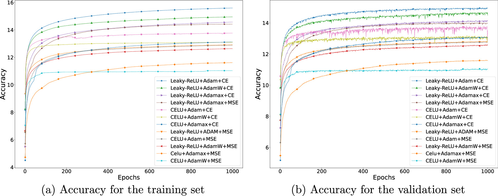