Dynamic & norm-based weights to normalize imbalance in back-propagated gradients of physics-informed neural networks

Consider the following initial and boundary value problem:

$$\begin{eqnarray}&&\displaystyle \frac{\partial }{\partial t}{\boldsymbol{u}}\left(t,{\boldsymbol{x}}\right)={ \mathcal F }\left[{\boldsymbol{u}}\left(t,{\boldsymbol{x}}\right);{\boldsymbol{\mu }}\right]\qquad \qquad \qquad \left(t,{\boldsymbol{x}}\right)\in \left(0,T\right)\times {\rm{\Omega }}\end{eqnarray} \tag{ 1 }$$

$$\begin{eqnarray}&&{\boldsymbol{u}}\left(0,{\boldsymbol{x}}\right)={\boldsymbol{f}}\left({\boldsymbol{x}}\right)\qquad \qquad \qquad {\boldsymbol{x}}\in {\rm{\Omega }}\end{eqnarray} \tag{ 2 }$$

$$\begin{eqnarray}&&{\boldsymbol{u}}\left(t,{\boldsymbol{x}}\right)={\boldsymbol{g}}\left(t,{\boldsymbol{x}}\right)\qquad \qquad \qquad \left(t,{\boldsymbol{x}}\right)\in \left(0,T\right)\times \partial {{\rm{\Omega }}}_{{\rm{D}}}\end{eqnarray} \tag{ 3 }$$

where Ω is the target domain (${\rm{\Omega }}\subset {{\mathbb{R}}}^{d}$, d is the dimension), ∂Ω_D is the Dirichlet boundary, and ${ \mathcal F }\left[\cdot ;{\boldsymbol{\mu }}\right]$ is a non-linear differential operator parameterized by μ (for instance, diffusion rate in diffusion equation, or viscosity in Navier–Stokes equation). Here we remark equation (3) corresponds to Dirichlet boundary condition, and other boundary conditions can be imposed as well (e.g. for Neumann boundary condition, $\tfrac{\partial }{\partial {\boldsymbol{n}}}{\boldsymbol{u}}={\boldsymbol{h}}$, with unit normal vector n on Neumann boundary, ∂Ω_N). PINN [17] first approximates the solution u by a neural network $\hat{{\boldsymbol{u}}}\left(t,{\boldsymbol{x}};{\boldsymbol{\theta }}\right)$ ( θ is a parameter vector) [34]. For a neural network whose input is ${\bf{x}}\left(=\left(t,{\boldsymbol{x}}\right)\in {{\mathbb{R}}}^{{f}_{\mathrm{in}}}\right)$ and output is $\hat{{\bf{y}}}\left(=\hat{{\boldsymbol{u}}}\in {{\mathbb{R}}}^{{f}_{\mathrm{out}}}\right)$,its forward propagation ${{\bf{z}}}^{(l)}\left(\in {{\mathbb{R}}}^{{f}_{\mathrm{hidden}}^{(l)}}\right)$ (l = 1, 2,...L) can be written as:

$$\begin{eqnarray}&&{{\bf{z}}}^{(l)}={\sigma }^{(l)}\left({{\bf{W}}}^{(l)}{{\bf{z}}}^{(l-1)}+{{\bf{b}}}^{(l)}\right)\end{eqnarray} \tag{ 4 }$$

where z⁽⁰⁾=x, ${{\bf{z}}}^{(L)}=\hat{{\bf{y}}}$, and σ^(l)( · ) is the activation function (element-wise non-linearity). ${{\bf{W}}}^{(l)}\left(\in {{\mathbb{R}}}^{{f}_{\mathrm{hidden}}^{(l)}\times {f}_{\mathrm{hidden}}^{(l-1)}}\right)$ and ${{\bf{b}}}^{(l)}\left(\in {{\mathbb{R}}}^{{f}_{\mathrm{hidden}}^{(l)}}\right)$ are weights and biases that form ${\boldsymbol{\theta }}\left(={\{{{\bf{W}}}^{(l)},{{\bf{b}}}^{(l)}\}}_{l=1}^{L}\right)$. The network parameter θ is then trained by minimizing the following loss function:

$$\begin{eqnarray}&&{ \mathcal L }({\boldsymbol{\theta }})={{ \mathcal L }}_{\mathrm{PDE}}({\boldsymbol{\theta }})+{{ \mathcal L }}_{\mathrm{IC}}({\boldsymbol{\theta }})+{{ \mathcal L }}_{\mathrm{BC}}({\boldsymbol{\theta }})\left(+{{ \mathcal L }}_{\mathrm{Data}}({\boldsymbol{\theta }})\right)\end{eqnarray} \tag{ 5 }$$

where ${{ \mathcal L }}_{\mathrm{PDE}}$ represents a loss term to penalize PDE residual, ${{ \mathcal L }}_{\mathrm{IC}}$ and ${{ \mathcal L }}_{\mathrm{BC}}$ are associated with IC/BC, respectively. ${{ \mathcal L }}_{\mathrm{Data}}$ could be added to equation (5) if there are available data within Ω. For typical problems, each term takes the following form:

$$\begin{eqnarray}&&{{ \mathcal L }}_{\mathrm{PDE}}=\displaystyle \frac{1}{{N}_{\mathrm{PDE}}}\displaystyle \sum _{i}^{{N}_{\mathrm{PDE}}}{\left|\displaystyle \frac{\partial }{\partial t}{\hat{{\boldsymbol{u}}}}_{i}-{ \mathcal F }\left[{\hat{{\boldsymbol{u}}}}_{i};{\boldsymbol{\mu }}\right]\right|}^{2}\end{eqnarray} \tag{ 6 }$$

$$\begin{eqnarray}&&{{ \mathcal L }}_{\mathrm{IC}}=\displaystyle \frac{1}{{N}_{\mathrm{IC}}}\displaystyle \sum _{i}^{{N}_{\mathrm{IC}}}{\left|{\hat{{\boldsymbol{u}}}}_{i}-{\boldsymbol{f}}({{\boldsymbol{x}}}_{i})\right|}^{2}\end{eqnarray} \tag{ 7 }$$

$$\begin{eqnarray}&&{{ \mathcal L }}_{\mathrm{BC}}=\displaystyle \frac{1}{{N}_{\mathrm{BC}}}\displaystyle \sum _{i}^{{N}_{\mathrm{BC}}}{\left|{\hat{{\boldsymbol{u}}}}_{i}-{\boldsymbol{g}}({t}_{i},{{\boldsymbol{x}}}_{i})\right|}^{2}\end{eqnarray} \tag{ 8 }$$

$$\begin{eqnarray}&&{{ \mathcal L }}_{\mathrm{Data}}=\displaystyle \frac{1}{{N}_{\mathrm{Data}}}\displaystyle \sum _{i}^{{N}_{\mathrm{Data}}}{\left|{\hat{{\boldsymbol{u}}}}_{i}-{\boldsymbol{u}}({t}_{i},{{\boldsymbol{x}}}_{i})\right|}^{2}\end{eqnarray} \tag{ 9 }$$

where ${\hat{{\boldsymbol{u}}}}_{i}=\hat{{\boldsymbol{u}}}({t}_{i},{{\boldsymbol{x}}}_{i};{\boldsymbol{\theta }})$. In the present work, we assume that the physical parameter μ is known; hence, we focus on forward problems. If μ is unknown and any data are available to define equation (9), one can extend PINNs to inverse problems as well [17, 18, 35]. One can rewrite equation (5) in the general form as follows.

$$\begin{eqnarray}&&{ \mathcal L }\left({\boldsymbol{\theta }}\right)=\displaystyle \sum _{j}{{ \mathcal L }}_{j}\left({\boldsymbol{\theta }}\right)\end{eqnarray} \tag{ 10 }$$

where ${{ \mathcal L }}_{j}$ represents the loss component associated with PDE residual, IC, BC, etc. In general, θ is learned with a gradient decent method or one of its variants, such as [33, 36].

$$\begin{eqnarray}\begin{array}{rcl}{{\boldsymbol{\theta }}}^{(n+1)} & = & {{\boldsymbol{\theta }}}^{(n)}-{\eta }^{(n)}{{\rm{\nabla }}}_{{\boldsymbol{\theta }}}{ \mathcal L }\left({{\boldsymbol{\theta }}}^{(n)}\right)\\ & = & {{\boldsymbol{\theta }}}^{(n)}-{\eta }^{(n)}\displaystyle \sum _{j}{{\rm{\nabla }}}_{{\boldsymbol{\theta }}}{{ \mathcal L }}_{j}\left({{\boldsymbol{\theta }}}^{(n)}\right)\end{array}\end{eqnarray} \tag{ 11 }$$

where θ ⁽ⁿ⁾ and η⁽ⁿ⁾ are the parameter and the learning rate at the n-th epoch, respectively.

2.2.1. Static weight tuning

It is natural to extend the equation (10) by introducing relative weights to each component.

$$\begin{eqnarray}&&{ \mathcal L }\left({\boldsymbol{\theta }}\right)=\displaystyle \sum _{j}{\lambda }_{j}{{ \mathcal L }}_{j}\left({\boldsymbol{\theta }}\right)\end{eqnarray} \tag{ 12 }$$

where ${\lambda }_{j}(\in {{\mathbb{R}}}^{+})$ is a weight assigned to ${{ \mathcal L }}_{j}$, controlling the relative importance of ${{ \mathcal L }}_{j}$ to ${{ \mathcal L }}_{k}$ (for j ≠ k). Accordingly, gradient descent is rewritten as follows.

$$\begin{eqnarray}&&{{\boldsymbol{\theta }}}^{(n+1)}={{\boldsymbol{\theta }}}^{(n)}-{\eta }^{(n)}\displaystyle \sum _{j}{\lambda }_{j}{{\rm{\nabla }}}_{{\boldsymbol{\theta }}}{{ \mathcal L }}_{j}\left({{\boldsymbol{\theta }}}^{(n)}\right)\end{eqnarray} \tag{ 13 }$$

It is critical to choose an appropriate λ_j as it drastically affects the learning procedure and the performance of PINNs without any change in the architecture [24, 26, 37]. Many works (e.g. [19, 24, 35, 37]) often treat λ_j as hyper-parameters, which are fixed prior to training, hence, we refer to such weight tuning as 'static weight tuning'. In many cases, the choice of λ_j is problem specific, making the cost to find the optimal λ_j prohibitively expensive, although several techniques can exploit these difficulties [38, 39].

2.2.2. Dynamic weight tuning

Back-propagated gradients often provide beneficial information to understand the training process of neural networks [40, 41]. Wang et al [31] have shown that regular training with equation (10) often causes an imbalance in multiple parameter gradients, ${{\rm{\nabla }}}_{{\boldsymbol{\theta }}}{{ \mathcal L }}_{\mathrm{PDE}}$, ${{\rm{\nabla }}}_{{\boldsymbol{\theta }}}{{ \mathcal L }}_{\mathrm{IC}}$, ${{\rm{\nabla }}}_{{\boldsymbol{\theta }}}{{ \mathcal L }}_{\mathrm{BC}}$, etc. Observing that ${{\rm{\nabla }}}_{{\boldsymbol{\theta }}}{{ \mathcal L }}_{\mathrm{PDE}}$ often dominates other gradients, they consider some positive weight ${\lambda }_{j}^{(n)}(\in {{\mathbb{R}}}^{+})$ which approximately satisfies the following.

$$\begin{eqnarray}&&\max \{| {{\rm{\nabla }}}_{{\boldsymbol{\theta }}}{{ \mathcal L }}_{\mathrm{PDE}}\left({{\boldsymbol{\theta }}}^{(n)}\right)| \}={\lambda }_{j}^{(n)}| {{\rm{\nabla }}}_{{\boldsymbol{\theta }}}{{ \mathcal L }}_{j}\left({{\boldsymbol{\theta }}}^{(n)}\right)| \end{eqnarray} \tag{ 14 }$$

Equation (14) then yields the following dynamic weight.

$$\begin{eqnarray}&&{\hat{\lambda }}_{j}^{(n)}=\displaystyle \frac{\max \{| {{\rm{\nabla }}}_{{\boldsymbol{\theta }}}{{ \mathcal L }}_{\mathrm{PDE}}\left({{\boldsymbol{\theta }}}^{(n)}\right)| \}}{{\lambda }_{j}^{(n-1)}\overline{| {{\rm{\nabla }}}_{{\boldsymbol{\theta }}}{{ \mathcal L }}_{j}\left({{\boldsymbol{\theta }}}^{(n)}\right)| }}\end{eqnarray} \tag{ 15 }$$

$$\begin{eqnarray}&&{\lambda }_{j}^{(n)}=\beta {\lambda }_{j}^{(n-1)}+(1-\beta ){\hat{\lambda }}_{j}^{(n)}\end{eqnarray} \tag{ 16 }$$

where ${\lambda }_{j}^{(n)}$ is the relative weight assigned to ${{ \mathcal L }}_{j}$ at n-th epoch (${\lambda }_{j}^{(n)}$ replaces λ_j in equation (13)). ∣ · ∣ is the element-wise absolute value, $\overline{\left(\cdot \right)}$ is the arithmetic mean, $\beta \left(\in [0,1)\right)$ is the exponential decay rate, and ${\lambda }_{j}^{(0)}$ is chosen as ${\lambda }_{j}^{(0)}=1$. Although equations (15) is the weight directly obtained from (14), they apply exponential decay to smooth out the noisy behavior of gradient descent methods (equation (16)). In this method, the weights are determined by the ratio of the maximum value of $| {{\rm{\nabla }}}_{{\boldsymbol{\theta }}}{{ \mathcal L }}_{\mathrm{PDE}}|$ to the average value of $| {{\rm{\nabla }}}_{{\boldsymbol{\theta }}}{{ \mathcal L }}_{j}|$, hence we refer to it as 'Maximum Average PINNs (MA-PINNs)'. The update interval for these relative weights is arbitrary, but it is recommended that it be large enough to avoid an additional computational cost increase, especially when the network is deep and wide.

Similarly, Maddu et al [32] considered a positive scalar to equalize the variance of each gradient. Assuming that gradients are normally distributed (${{\rm{\nabla }}}_{{\boldsymbol{\theta }}}{{ \mathcal L }}_{\mathrm{PDE}}\sim { \mathcal N }\left({m}_{\mathrm{PDE}},{v}_{\mathrm{PDE}}^{2}\right)$ and ${{\rm{\nabla }}}_{{\boldsymbol{\theta }}}{{ \mathcal L }}_{j}\sim { \mathcal N }\left({m}_{j},{v}_{j}^{2}\right)$, where ${ \mathcal N }\left(m,{v}^{2}\right)$ is a normal distribution with mean m and variance v²), we have ${\lambda }_{j}{{\rm{\nabla }}}_{{\boldsymbol{\theta }}}{{ \mathcal L }}_{j}\sim { \mathcal N }\left({\lambda }_{j}{m}_{j},{\lambda }_{j}^{2}{v}_{j}^{2}\right)$. For the variance of ${{\rm{\nabla }}}_{{\boldsymbol{\theta }}}{{ \mathcal L }}_{\mathrm{PDE}}$ and that of ${{\rm{\nabla }}}_{{\boldsymbol{\theta }}}{{ \mathcal L }}_{j}$ be (approximately) equal at n-th epoch, we have:

$$\begin{eqnarray}&&v\left[{{\rm{\nabla }}}_{{\boldsymbol{\theta }}}{{ \mathcal L }}_{\mathrm{PDE}}({{\boldsymbol{\theta }}}^{(n)})\right]={\left({\lambda }_{j}^{(n)}\right)}^{2}v\left[{{\rm{\nabla }}}_{{\boldsymbol{\theta }}}{{ \mathcal L }}_{j}({{\boldsymbol{\theta }}}^{(n)})\right]\end{eqnarray} \tag{ 17 }$$

which gives the following dynamic weight.

$$\begin{eqnarray}&&{\hat{\lambda }}_{j}^{(n)}=\displaystyle \frac{s\left[{{\rm{\nabla }}}_{{\boldsymbol{\theta }}}{{ \mathcal L }}_{\mathrm{PDE}}({{\boldsymbol{\theta }}}^{(n)})\right]}{s\left[{{\rm{\nabla }}}_{{\boldsymbol{\theta }}}{{ \mathcal L }}_{j}({{\boldsymbol{\theta }}}^{(n)})\right]}\end{eqnarray} \tag{ 18 }$$

where $s\left[\cdot \right]$ is the sample standard deviation (equation (18) is valid when we have only one set of PDEs as ${{ \mathcal L }}_{\mathrm{PDE}}$ has the highest order of derivatives; see [32] for the generalized form with multiple sets of governing PDEs). Applying exponential decay, equation (16) is performed after equation (18). This weight tuning scheme keeps the variance of each gradient component approximately equal, and such weights are proportional to the inverse of the square root of the Dirichlet energy of each loss component. Therefore, we refer to this method as 'Inverse Dirichlet PINNs (ID-PINNs)'.

Equation (23) smooths the weight defined in equation (22). As one can see, the choice of β plays a crucial role; small β (β → 0) gives a wild change in ${\lambda }_{j}^{(n)}$, while large β (β → 1) makes a gradual change. Although our preliminary numerical experiments find that large β provides stable training of PINNs, such β causes a strong bias toward its initial values. In fact, β = 1 does not update ${\lambda }_{j}^{(n)}$, hence there is no difference from the standard PINN. Here, motivated by [33], we consider the initialization bias of ${\lambda }_{j}^{(n)}$. Recursive evaluation of equation (23) gives the following.

$$\begin{eqnarray}&&x{\lambda }_{j}^{(n)}={\beta }^{n}{\lambda }_{j}^{(0)}+\left(1-\beta \right)\displaystyle \sum _{k=1}^{n}{\beta }^{n-k}{\hat{\lambda }}_{j}^{(k)}\end{eqnarray} \tag{ 24 }$$

with its initial value ${\lambda }_{j}^{(0)}$. Taking expectation of both hand side, we have:

$$\begin{eqnarray}\begin{array}{rcl}{\mathbb{E}}\left[{\lambda }_{j}^{(n)}\right] & = & {\beta }^{n}{\lambda }_{j}^{(0)}+\left(1-\beta \right){\mathbb{E}}\left[\displaystyle \sum _{k=1}^{n}{\beta }^{n-k}{\hat{\lambda }}_{j}^{(k)}\right]\\ & \approx & {\beta }^{n}{\lambda }_{j}^{(0)}+\left(1-\beta \right)\displaystyle \sum _{k=1}^{n}{\beta }^{n-k}{\mathbb{E}}\left[{\hat{\lambda }}_{j}^{(n)}\right]\\ & = & {\beta }^{n}{\lambda }_{j}^{(0)}+\left(1-{\beta }^{n}\right){\mathbb{E}}\left[{\hat{\lambda }}_{j}^{(n)}\right]\end{array}\end{eqnarray} \tag{ 25 }$$

where we used the approximation under the assumption that the change of ${\hat{\lambda }}_{j}^{(k)}$ is relatively small over different epochs, and the property of geometric progression. With the decay rate β set to 0 ≤ β < 1, βⁿ → 0 with increasing n (training epoch). However, in the early stage of the training, ${\lambda }_{j}^{(n)}$ is considered to be biased toward its initial value ${\lambda }_{j}^{(0)}$. To remove it, one can initialize ${\lambda }_{j}^{(0)}=0$ and introduce bias-corrected weight ${\tilde{\lambda }}_{j}^{(n)}$ [33] as:

$$\begin{eqnarray}&&{\tilde{\lambda }}_{j}^{(n)}=\displaystyle \frac{{\lambda }_{j}^{(n)}}{1-{\beta }^{n}}\end{eqnarray} \tag{ 26 }$$

where ${\tilde{\lambda }}_{j}^{(n)}$ is applied to ${{ \mathcal L }}_{j}$ in place of ${\lambda }_{j}^{(n)}$. The effect of this bias correction is discussed in section 4.4.

We first consider the following 1D Burgers' equation, which has been widely studied as a benchmark problem for PINNs [17, 27, 29, 45]. Burgers' equation is one of the fundamental convection–diffusion systems and can be considered as a simplified Navier–Stokes equation with a sharp solution transition.

$$\begin{eqnarray}&&\displaystyle \frac{\partial u}{\partial t}+(u\cdot {\rm{\nabla }})u=\nu {{\rm{\nabla }}}^{2}u\end{eqnarray} \tag{ 28 }$$

$$\begin{eqnarray}&&u(0,x)=-\sin (\pi x)\end{eqnarray} \tag{ 29 }$$

$$\begin{eqnarray}&&u(t,\pm 1)=0\end{eqnarray} \tag{ 30 }$$

where u = u(t, x), t ∈ [0, 1], x ∈ [ − 1, 1], and ν is the viscosity set to ν = 0.01/π. For training, we set L = 9, ${f}_{\mathrm{hidden}}^{(l)}=20$, and the number of training points as N_PDE = 10, 000, N_IC = 100, N_BC = 200, which are consistent with [17, 29]. We performed full-batch training for 30,000 epochs.

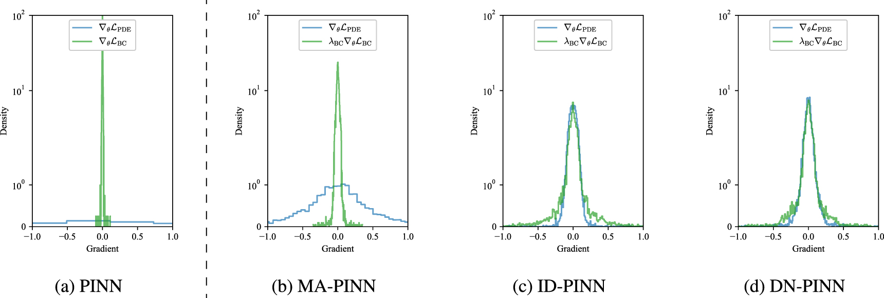
Table 1 summarizes the results obtained by the baseline PINN, MA-PINN, ID-PINN, and the proposed DN-PINN. For β = 0.9, we observe MA-PINN achieves the best performance among variants, while for β = 0.99, ID-PINN appears to be the best. Figure 2 shows the inference result and the absolute error of the baseline PINN and variants. Figure 3 shows the back-propagated gradient distribution of each method after training. In figure 2, we observe that the baseline PINN is able to learn the overall solution but still struggles to properly capture the initial condition, especially in t ∈ [0, 0.4]. This may be explained in figure 3, which shows that for PINN, ${{\rm{\nabla }}}_{{\boldsymbol{\theta }}}{{ \mathcal L }}_{\mathrm{IC}}$ and ${{\rm{\nabla }}}_{{\boldsymbol{\theta }}}{{ \mathcal L }}_{\mathrm{BC}}$ have relatively vanished compared to ${{\rm{\nabla }}}_{{\boldsymbol{\theta }}}{{ \mathcal L }}_{\mathrm{PDE}}$. On the contrary, again in figure 2, we see a small discrepancy between the reference and the inference solution for MA-PINN, ID-PINN, and DN-PINN, including t ∈ [0, 0.4] region. In addition, figure 3 illustrates that each gradient is evenly distributed for the dynamic weighting schemes presented, which explains a small error near the t = 0. One drawback of dynamic weighting schemes is their additional computational cost. Table 1 shows that all dynamic weighting schemes increase the training time from the baseline PINN. However, an increase of 30% ∼40% is reasonable considering the elimination of manual parameter search and the improvement obtained by introducing dynamic weights.

Zoom In Zoom Out Reset image size

Zoom In Zoom Out Reset image size

Table 1.  1D Burgers' equation. Mean of relative L² error (±standard error) for 10 runs and training time for 30,000 epochs of full-batch training (+ increase from the baseline PINN in percentile).

Method	β	Rel. L2 Err. (×10−3)	Training time (s)
PINN [17]	⋯	9.26 (±1.36)	526.55
MA-PINN [31]	0.9	7.68 (±0.74)	701.31 (+33%)
ID-PINN [32]	0.9	10.26 (±2.62)	705.08 (+34%)
DN-PINN (Ours)	0.9	12.70 (±2.25)	703.61 (+34%)
MA-PINN [31]	0.99	8.58 (±1.79)	704.95 (+34%)
ID-PINN [32]	0.99	7.12 (±1.28)	704.98 (+34%)
DN-PINN (Ours)	0.99	7.49 (±1.12)	703.45 (+34%)

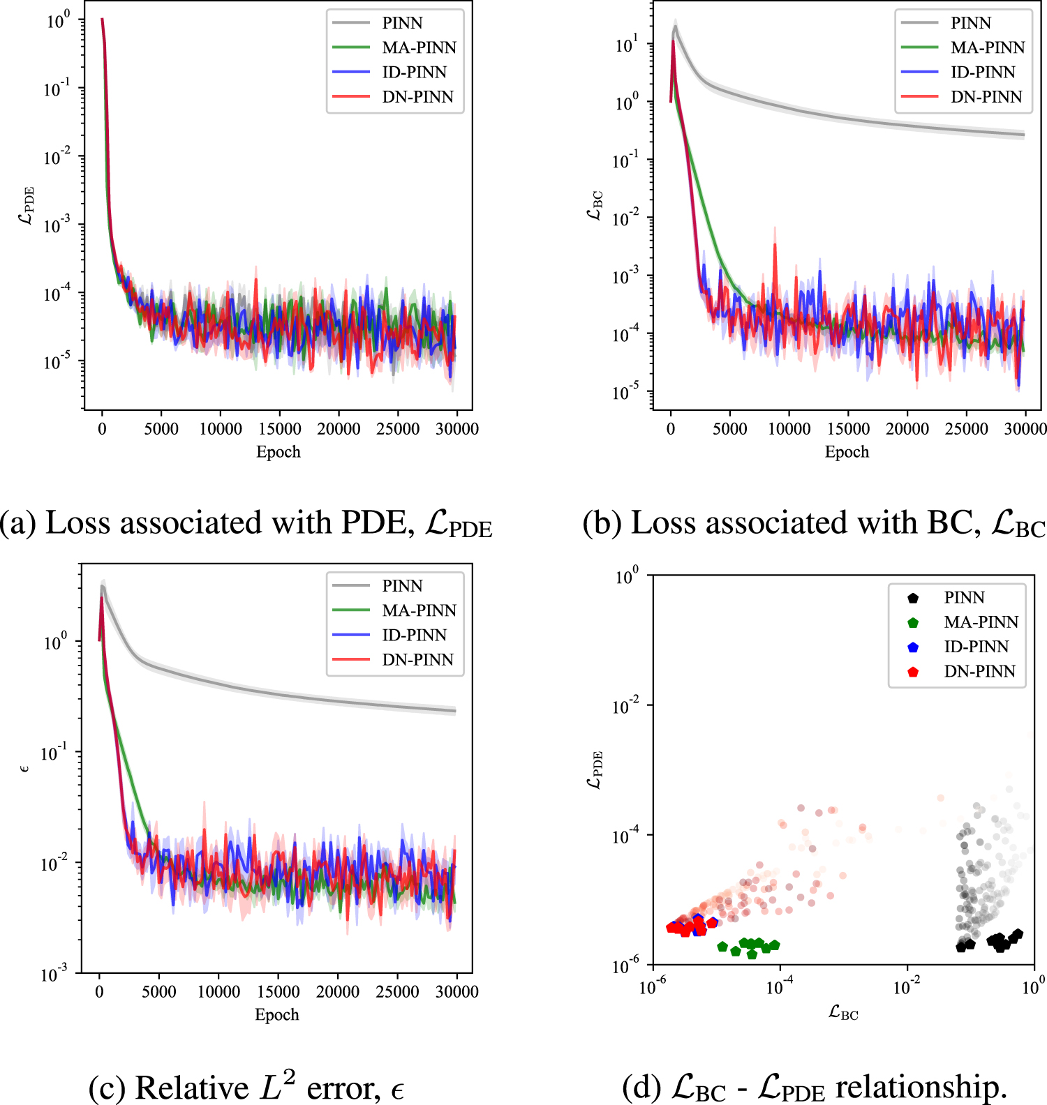
To further investigate the learning process of PINNs, in figure 4, we plot the individual loss ${{ \mathcal L }}_{\mathrm{PDE}}$, ${{ \mathcal L }}_{\mathrm{IC}}$, ${{ \mathcal L }}_{\mathrm{PDE}}$, relative L² error, , and relationship between loss components (loss values are normalized by its initial value to realize the convergence rate). Here, the relative weights of MA-PINN, ID-PINN, and DN-PINN are removed in figure 4 for comparison with PINN. For ${{ \mathcal L }}_{\mathrm{IC}}$–${{ \mathcal L }}_{\mathrm{PDE}}$ relationship and ${{ \mathcal L }}_{\mathrm{BC}}$-${{ \mathcal L }}_{\mathrm{PDE}}$ relationship (figures 4(e) and 4(f)), we plot the lowest loss achieved by 10 runs with pentagons and plot the training trajectories of PINN and DN-PINN (lighter color, earlier stage of training; darker color, later stage, only the trajectories of PINN and DN-PINN are shown for visualization purpose, but we find that those of MA-PINN and ID-PINN are similar to DN-PINN). Figure 4 (e) shows that MA-PINN, ID-PINN, and DN-PINN, compared to the baseline PINN, are possible to reduce ${{ \mathcal L }}_{\mathrm{IC}}$ even better, while being unable to lower ${{ \mathcal L }}_{\mathrm{PDE}}$ any further. This result is fairly natural; as is well known on the Pareto front, PINNs (or many multi-objective optimizations) cannot further reduce one loss component without increasing another [26]. Again, from figures 3, it is evident that PINN tends to greatly respect ${{ \mathcal L }}_{\mathrm{PDE}}$ and decrease it rapidly while paying little attention to ${{ \mathcal L }}_{\mathrm{IC}}$, resulting in a large accumulation of errors in t ∈ [0, 0.4]. MA-PINN, ID-PINN, and DN-PINN, on the other hand, successfully avoid the Pareto optimum where the standard PINN is trapped due to the effect of relative weights λ_IC. Though they cannot reduce ${{ \mathcal L }}_{\mathrm{PDE}}$ as much as PINN does, they are able to lower ${{ \mathcal L }}_{\mathrm{IC}}$ in return. As a consequence, they yield a lower relative L² error compared to the baseline PINN. For the ${{ \mathcal L }}_{\mathrm{PDE}}$ - ${{ \mathcal L }}_{\mathrm{BC}}$ relationship, we find very little difference among them. This indicates that the loss component associated with the boundary condition is of relatively small importance, as ${{ \mathcal L }}_{\mathrm{BC}}$ plateaus at almost the same level for all methods (see figure 4(f)).

Zoom In Zoom Out Reset image size

From this comparative study, although we did not find a significant improvement over the baseline PINN for this problem, we stress that all dynamic weighting schemes were successful in evenly distributing multiple loss gradients, as illustrated in figure 3, and changed the learning dynamics of the PINNs as shown in figure 4. Besides, they only require a reasonable computational cost for the improvement, although it varies depending on the choice of τ (we chose τ = 10 in this study).

As another evaluation and comparison of PINN and variants, we next consider the 2D Poisson equation. The Poisson equation is closely related to many natural science and engineering problems, such as electromagnetics and fluid mechanics.

$$\begin{eqnarray}&&{{\rm{\nabla }}}^{2}u=q(x,y)\end{eqnarray} \tag{ 31 }$$

$$\begin{eqnarray}&&u(x,0)=u(x,1)=0\end{eqnarray} \tag{ 32 }$$

$$\begin{eqnarray}&&u(0,y)=u(1,y)=\sin (\omega y)\end{eqnarray} \tag{ 33 }$$

where u = u(x, y), x ∈ [0, 1], y ∈ [ − 1, 1]. The analytical solution for equation (31) can be fabricated as $u=\cos (\omega x)\sin (\omega y)$ with the forcing term $q=-2{\omega }^{2}\cos (\omega x)\sin (\omega y)$. ω is a parameter to control the oscillation frequency of the solution, set as ω = 4π. For this problem, we used a network with L = 5, ${f}_{\mathrm{hidden}}^{(l)}=50$, N_PDE = 2, 500, N_BC = 400, and performed full-batch training for 30,000 epochs [32].

Table 2 summarizes the results by PINN, MA-PINN, ID-PINN, and DN-PINN. We find that DN-PINN slightly outperforms other variants for both β = 0.9 and 0.99, followed by ID-PINN, MA-PINN, and PINN, but the performance of DN-PINN and that of ID-PINN are almost identical. Clearly, the baseline PINN works poorly even on this simple problem. In particular, figure 5 shows that PINN accumulates a large error near the boundaries, while reducing the error near the geometric center of the domain. Similar to the previous example, this behavior can be interpreted by looking at the back-propagated gradient distribution and the convergence property of the loss function. In figure 6(a), for PINN, it can be seen that the parameter gradient of the PDE residual ${{\rm{\nabla }}}_{{\boldsymbol{\theta }}}{{ \mathcal L }}_{\mathrm{PDE}}$ is widely distributed, helping to reduce ${{ \mathcal L }}_{\mathrm{PDE}}$. However, the gradient of the boundary condition ${{\rm{\nabla }}}_{{\boldsymbol{\theta }}}{{ \mathcal L }}_{\mathrm{BC}}$ is concentrated near zero and therefore the decrease of ${{ \mathcal L }}_{\mathrm{BC}}$ is slowed down (see figure 7(d)). Note that in figure 7(d), we plot the lowest loss achieved by 10 runs with pentagons and plot the training trajectories of PINN and DN-PINN (lighter color, earlier stage of training; darker color, later stage, only the trajectories of PINN and DN-PINN are shown). As a result, the baseline PINN is driven to provide a general solution rather than a specific solution to the given boundary value problem. On the other hand, the effect of dynamic weight tuning methods is evident in this problem. In particular, MA-PINN greatly reduces the error near the boundaries, resulting in a relative L² error that is nearly 100 times smaller than that of PINN. From figure 7, we can see that MA-PINN has successfully decreased ${{ \mathcal L }}_{\mathrm{BC}}$ as well as ${{ \mathcal L }}_{\mathrm{PDE}}$. However, in figure 6, we observe that MA-PINN still struggles to alleviate the gradient imbalance. On the contrary, ID-PINN and DN-PINN successfully reduce the error throughout the domain as shown in figure 5, while distributing ${{\rm{\nabla }}}_{{\boldsymbol{\theta }}}{{ \mathcal L }}_{\mathrm{PDE}}$ and ${{\rm{\nabla }}}_{{\boldsymbol{\theta }}}{{ \mathcal L }}_{\mathrm{BC}}$ equally (figures 6(c) and (d)). Similarly to the previous 1D Burgers problem, the additional computational cost of MA-PINN, ID-PINN, and DN-PINN remains small (∼30%), while the gain in accuracy is ∼100x.

Zoom In Zoom Out Reset image size

Zoom In Zoom Out Reset image size

Zoom In Zoom Out Reset image size

Table 2.  2D Poisson equation. Mean of relative L² error (±standard error) for 10 runs and training time for 30,000 epochs of full-batch training (+ increase from the baseline PINN in percentile).

Method	β	Rel. L2 Err. (×10−3)	Training time (s)
PINN [17]	⋯	232.29 (±19.18)	245.30
MA-PINN [31]	0.9	2.05 (±0.11)	297.25 (+21%)
ID-PINN [32]	0.9	1.47 (±0.11)	300.04 (+22%)
DN-PINN (Ours)	0.9	1.41 (±0.11)	298.10 (+22%)
MA-PINN [31]	0.99	2.06 (±0.19)	299.77 (+22%)
ID-PINN [32]	0.99	1.13 (±0.11)	298.66 (+22%)
DN-PINN (Ours)	0.99	1.11 (±0.11)	297.92 (+21%)

To examine the learning process of each method, figure 7 illustrates the relationship between ${{ \mathcal L }}_{\mathrm{PDE}}$ and ${{ \mathcal L }}_{\mathrm{BC}}$, loss values of ${{ \mathcal L }}_{\mathrm{PDE}}$ and ${{ \mathcal L }}_{\mathrm{BC}}$ during training (normalized by their initial values to realize the convergence rate). Evidently, PINN can reduce ${{ \mathcal L }}_{\mathrm{PDE}}$, but it fails to deal with ${{ \mathcal L }}_{\mathrm{BC}}$ even with a long training time. In particular, the loss associated with the boundary condition ${{ \mathcal L }}_{\mathrm{BC}}$ remains 4∼5 orders of magnitude greater than the loss of PDE residual ${{ \mathcal L }}_{\mathrm{PDE}}$. These observations imply that regular PINN training is biased to satisfy the governing PDE with little attention is paid to the imposed boundary condition. Figure 7 shows that MA-PINN effectively reduces both ${{ \mathcal L }}_{\mathrm{PDE}}$ and ${{ \mathcal L }}_{\mathrm{BC}}$. As a result, it achieves an improvement of almost 2 orders of magnitude over the baseline PINN in relative L² error, as summarized in table 2. Moreover, ID-PINN and DN-PINN achieve even lower ${{ \mathcal L }}_{\mathrm{BC}}$ than MA-PINN. We consider this to be due to the aforementioned incomplete alleviation of the gradient imbalance found in figure 6, while the gradients of ${{ \mathcal L }}_{\mathrm{PDE}}$ and ${{ \mathcal L }}_{\mathrm{BC}}$ in ID-PINN and DN-PINN are equally distributed. Consequently, their inference results are more accurate.

A comparative study on this problem suggests that, in some cases, the baseline PINN may rely heavily on the PDE residual for its training while little attention is drawn to the given boundary conditions, as reported in [26, 31, 32]. These symptoms are considered due to an unequal gradient distribution over multiple objectives, as illustrated in figure 6. We observe that MA-PINN is very effective in avoiding this problem, but it still suffers from the imbalance. We also find that ID-PINN and DN-PINN could be powerful weight tuning strategies in evenly distributing multiple gradient components without being harmed by the gradient imbalance.

As the last example, we consider the following 1D Allen-Cahn equation, which is reported to be challenging for the baseline PINN [24]. The Allen-Cahn equation is a class of reaction-diffusion systems of which application spans from material science to biology [46, 47].

$$\begin{eqnarray}&&\displaystyle \frac{\partial u}{\partial t}={a}_{1}{{\rm{\nabla }}}^{2}u+{a}_{2}(u-{u}^{3})\end{eqnarray} \tag{ 34 }$$

$$\begin{eqnarray}&&u(0,x)={x}^{2}\cos (\pi x)\end{eqnarray} \tag{ 35 }$$

$$\begin{eqnarray}&&u(t,-1)=u(t,1)\end{eqnarray} \tag{ 36 }$$

$$\begin{eqnarray}&&{\rm{\nabla }}u(t,-1)={\rm{\nabla }}u(t,1)\end{eqnarray} \tag{ 37 }$$

where u = u(t, x), t ∈ [0, 1], x ∈ [ − 1, 1]. a₁ and a₂ are diffusion and reaction rates, respectively, and are chosen as a₁ = 0.0001 and a₂ = 5. As for the neural network architecture and problem setup, we chose L = 5, ${f}_{\mathrm{hidden}}^{(l)}=128$, N_PDE = 20, 000, N_IC = 512, N_BC = 200 in accordance with [24]. We performed mini-batch training for 50,000 epochs with batch size 4,096. Here, mini-batching is only applied to PDE residual computation since N_PDE ≫ N_IC, N_BC. Furthermore, we applied the aforementioned dynamic weights (MA-PINN, ID-PINN, and DN-PINN) only for the loss component of the initial condition, since the weights for the periodic boundary conditions have diverged for all methods.

Table 3 summarizes the results. For this problem, we again find ID-PINN and DN-PINN perform well better than MA-PINN or the baseline PINN. Furthermore, figure 8 shows the reference and inference solutions obtained by each method. For the result presented in 8, the baseline PINN is unable to capture the solution correctly, having a large discrepancy from the reference solution, especially in the sharp transition region, x ∈ [–0.5, 0.5], whereas dynamic weighting schemes are able to produce accurate solutions. To understand the cause of PINN failure, we again look at the back-propagated gradient distribution after training, as shown in figure 9. For the baseline PINN, the gradient of IC loss (${{\rm{\nabla }}}_{{\boldsymbol{\theta }}}{{ \mathcal L }}_{\mathrm{IC}}$) has a sharp distribution concentrated near zero compared to that of PDE loss (${{\rm{\nabla }}}_{{\boldsymbol{\theta }}}{{ \mathcal L }}_{\mathrm{PDE}}$), implying that IC training is drastically slowed down. On the contrary, dynamic weighting schemes distribute the gradient of IC loss more widely than PINN, indicating that IC training is enhanced. These results are consistent with [24, 29], where it has been found that high attention needs to be paid to the initial condition for learning this Allen-Cahn system. In figure 9, we also find MA-PINN behaves slightly differently from ID-PINN and DN-PINN. Particularly, MA-PINN distributes ${{\rm{\nabla }}}_{{\boldsymbol{\theta }}}{{ \mathcal L }}_{\mathrm{IC}}$ wider than ${{\rm{\nabla }}}_{{\boldsymbol{\theta }}}{{ \mathcal L }}_{\mathrm{PDE}}$, which is the opposite behavior from the previous example in 4.2. On the other hand, ID-PINN and DN-PINN achieve an even distribution of both gradient components. Combined with the observation in the previous example, MA-PINNs can be potentially unstable, underestimating or overestimating relative weights depending on the problems. Note that in figure 8, one can see that even dynamic weighting schemes cannot still accurately capture the sharp transition in t ∈ [0.5, 1.0]. It is well known that PINNs struggles to capture a sharp and discontinuous spatial change or a fast temporal evolution [48]. Especially for reaction-diffusion equations, sequential learning could potentially be effective for further improvement [24, 25]. As for training time, the extra cost introduced by dynamic weights was almost negligible for this problem, because we chose mini-batch training with long epochs.

Zoom In Zoom Out Reset image size

Zoom In Zoom Out Reset image size

Table 3.  1D Allen-Cahn equation. Mean of relative L² error (±standard error) for 10 runs and training time for 50,000 epochs with a batch size of 4,096 (+ increase from the baseline PINN in percentile).

Method	β	Rel. L2 err. (×10−2)	Training time (s)
PINN [17]	—	22.79 (±7.35)	8,121.97
MA-PINN [31]	0.9	3.30 (±0.19)	8,245.85 (+2%)
ID-PINN [32]	0.9	2.08 (±0.23)	8,246.31 (+2%)
DN-PINN (Ours)	0.9	1.60 (±0.19)	8,245.83 (+2%)
MA-PINN [31]	0.99	2.60 (±0.11)	8,246.16 (+2%)
ID-PINN [32]	0.99	1.50 (±0.17)	8,245.36 (+2%)
DN-PINN (Ours)	0.99	1.58 (±0.17)	8,246.36 (+2%)

To better understand the failure of PINN for this problem, figure 10 shows the loss components as a function of training epochs, relative L² error against the reference solution and the relationship between ${{ \mathcal L }}_{\mathrm{PDE}}$ and ${{ \mathcal L }}_{\mathrm{IC}}$, ${{ \mathcal L }}_{\mathrm{PDE}}$ and ${{ \mathcal L }}_{\mathrm{BC}}$. Again, in figures 10(e) and 10 (f), the loss values are normalized by their initial values and the relative weights are removed so we can compare with PINN. Pentagons indicate the lowest loss achieved by 10 independent runs, and only the trajectory of DN-PINN is shown here (the trajectories of MA-PINN and ID-PINN showed similar behavior). From figure 10(e), we find two clusters of PINN, one trapped around $\left({{ \mathcal L }}_{\mathrm{IC}},{{ \mathcal L }}_{\mathrm{PDE}}\right)=\left({10}^{-2},{10}^{-3}\right)$ and the other near $\left({{ \mathcal L }}_{\mathrm{IC}},{{ \mathcal L }}_{\mathrm{PDE}}\right)=\left({10}^{-4},{10}^{-4}\right)$. With the presence of the latter cluster, the former is considered to be local convergence solutions, and longer training could drive them closer to the latter cluster. Figure 11(a) shows 2 representatives from each cluster and (b) and (c) are the corresponding inference solutions. We can see that when PINN successfully reaches $\left({{ \mathcal L }}_{\mathrm{IC}},{{ \mathcal L }}_{\mathrm{PDE}}\right)=\left({10}^{-4},{10}^{-4}\right)$ then its inference solution is almost identical to those of dynamic weighting schemes (figure 11(b)), but it is also possible to reach $\left({{ \mathcal L }}_{\mathrm{IC}},{{ \mathcal L }}_{\mathrm{PDE}}\right)=\left({10}^{-2},{10}^{-3}\right)$ and yield very poor solution (figure 11(c)). We stress that they are independent runs with the exactly the same setup (e.g. depth, width, activation, learning rate, etc), but differ only in the random initialization (although taken from the same distribution), and therefore it is noteworthy that the baseline PINN may be able to capture the accurate solution without any weight tuning, but also has a high risk of failure.

Zoom In Zoom Out Reset image size

Zoom In Zoom Out Reset image size

While some of the PINN samples get stuck near $\left({{ \mathcal L }}_{\mathrm{IC}},{{ \mathcal L }}_{\mathrm{PDE}}\right)=\left({10}^{-2},{10}^{-3}\right)$ and have difficulty reducing ${{ \mathcal L }}_{\mathrm{IC}}$ after 10,000 epochs, MA-PINN, ID-PINN, and DN-PINN constantly lower both ${{ \mathcal L }}_{\mathrm{PDE}}$ and ${{ \mathcal L }}_{\mathrm{IC}}$ during training, being almost invariant to initialization randomness. This indicates that proper weight tuning allows for reliable training of PINNs. As a result, they successfully avoid the Pareto optimum in which PINN is trapped, as shown in figure 10(e). Although MA-PINN seems to be the fastest to start decreasing the loss of initial condition as can be seen in figure 10(b), it fails to completely resolve gradient imbalance as observed in figure 9(b). ID-PINN and DN-PINN achieve an almost equal distribution of ${{\rm{\nabla }}}_{{\boldsymbol{\theta }}}{{ \mathcal L }}_{\mathrm{IC}}$ and ${{\rm{\nabla }}}_{{\boldsymbol{\theta }}}{{ \mathcal L }}_{\mathrm{PDE}}$, providing an even better approximation than MA-PINN. As for the boundary condition loss ${{ \mathcal L }}_{\mathrm{BC}}$, we do not observe a significant difference among PINN and variants since we did not apply weights as stated above. Similarly to Burgers' problem, we consider this to mean that the loss of the loss associated with the initial condition ${{ \mathcal L }}_{\mathrm{IC}}$ is of great importance compared to ${{ \mathcal L }}_{\mathrm{BC}}$. In fact, applying the relative weight λ_IC barely changes the convergence trend of ${{ \mathcal L }}_{\mathrm{BC}}$, as illustrated in figures 10(c) and (f).

As discussed in 3.1, the choice of the exponential decay rate β is critical, but the bias correction in equation (26) can be a strong candidate to alleviate the initialization bias caused by the exponential decay. Here, we compare the results of DN-PINN without bias correction (equation (23)) and with bias correction (equation (26)). These additional experiments are performed as follows. For 1D Burgers and 1D Allen-Cahn problems, all settings (network architecture, optimizer, epochs, and batch-size) are unchanged from sections 4.1 and 4.3. For 2D Poisson problem, the neural network is trained for only 5,000 epochs (other settings are unchanged from section 4.2). This is because we have observed in section 4.2 that it quickly converges and begins to oscillate after the first few thousand epochs. We also vary the exponential decay rate as β = 0.9, 0.99, 0.999 while fixing the update interval to τ = 10.

Figure 12 shows the relative L² error, , of DN-PINN without and with bias correction, as a function of the training epochs. For 1D Burgers problem (figures 12(a)–(c)), increasing β appears to have a subtle effect on the DN-PINN training procedure without bias correction, as the convergence speed of the relative L² error, , are almost unchanged for β = 0.99 and β = 0.999. In contrast, for 2D Poisson (figures 12(d)–(f)) and 1D Allen-Cahn problems (figures 12(g)–(i)), DN-PINN without bias correction tends to require more training epochs to converge as β increases. This indicates that the weight update slows down and the effect of initialization bias becomes dominant when β is close to 1. On the other hand, DN-PINN with bias correction shows a nearly identical convergence speed for β = 0.99 and β = 0.999, suggesting that they are robust to the initialization bias caused by large β. Although it can be seen that, when β is relatively small (β = 0.9), the bias correction can sometimes make training unstable (see figures 12(a) and (g)), as our numerical experiments in sections 4.1, 4.2, 4.3 suggest, large β often provides better inference accuracy, and thus the combination of large β and bias correction can be a robust and versatile improvement. We also find that the training cost increment of introducing bias correction is negligible.

Zoom In Zoom Out Reset image size