
Abstract
Free space optical (FSO) wireless communication has emerged as a viable alternative to the existing fiber optics and radio frequency (RF) communications due to its ability to operate in unlicensed spectrum, offering huge data handling capacities and being cost effective with easy deployment. The underlying communication mechanism in the FSO link is based upon the laser beam propagation model. The propagating free space optical beam undergoes signal degradation due to refraction and diffraction caused by atmospheric turbulence measured by refractive index structure parameter (Cn2). In this work, a novel, robust analytical model for propagating Gaussian-beam through atmospheric turbulence is presented, by solving the space-fractional paraxial wave equation. We report analytical expressions for the intensity and long-term beam spreading of a Gaussian beam in terms of space-fractional parameter D, for the range 2 < D ≤ 3. This range of parameter D, defines the effective number of euclidean space corresponding to atmospheric turbulence levels faced by the propagating Gaussian beam in the FSO link. The results of the proposed fractional model and the existing models agreed well, therefore the D-dimensional parameter can be used to effectively express the value of refractive index structure parameter (Cn2). The classical values of Cn2 ranges form 10−13 to 10−16 for strong to weak fluctuations respectively. However, in fractional-dimension scale, these fluctuations can be express as D = 2.668 (strong fluctuations) to D = 2.999 (weak fluctuations). The ideal case of free space beam propagation can be expressed as D = 3, with no turbulence. Moreover, we have studied the fractional-dimension model performance for varying wavelengths. Further, based upon a practical example, we proposed a self-sustainable FSO link architecture to efficiently minimize the effect of weak and strong fluctuations on the propagating optical beam, based upon the D-dimension fractional parameter, hence ensuring reliability of FSO link.

Original content from this work may be used under the terms of the Creative Commons Attribution 4.0 licence. Any further distribution of this work must maintain attribution to the author(s) and the title of the work, journal citation and DOI.
1. Introduction
Free space optics (FSO) is considered superior to the existing radio frequency (RF), as it encompasses a wider bandwidth which has the possibility to become a viable remedy for limited spectrum currently offered by RF networks. FSO links provide data rates between 10 Mbps and 10 Gbps, making them suitable for usage as primary, secondary, or backup links [1]. FSO offers better security than current wireless and wired network systems since it is very resilient to interference. Unlicensed frequency spectrum, which can support high data rates, is an added benefit. FSO link has an edge over existing technologies due to its low hardware development cost and simplicity of use [2]. However, because the environment is a poor transmission medium for optical beams, outdoor FSO link performance is significantly impacted by optical signal loss caused by unfavourable weather conditions. The optical beam may encounter variations in signal intensity even in clear, visible conditions due to atmospheric turbulence. The air's refractive index along the course of propagation may vary because of inhomogeneity and variations in temperature and pressure values. The amount of air turbulence is measured using the refractive index structure parameter (Cn 2). Conventionally, the refractive index structure parameter has been measured using the Kolmogorov power law. The Kolmogorov theory defines the distribution of energy in turbulent cells contained in the inertial-range of eddies present in the atmosphere. Due to atmospheric turbulence, the diffraction of optical beam extends beyond that of free space. Theoretically the atmospheric turbulence models are categorized according to the intensity of fluctuations. These atmospheric fluctuations are distinguished as weak and strong based upon the Rytov parameter, which is the function of distance and Cn 2.
The atmospheric channel is a random medium by nature and its accurate modeling is complex to achieve. However some of the most common reported models to express the atmospheric turbulence include the log-normal distribution model [2], used to model weak atmospheric turbulence and the gamma-gamma distribution model [3] which is used to model moderate to strong atmospheric fluctuations. All these existing models are distinct in nature, with variable complexity level and limitations. There is a gap of a unified simple model that is capable enough to capture the turbulence in atmosphere at all given levels.
The idea of fractional-dimensional space has lately been used to effectively examine physical phenomena in complex objects that are anisotropic and nonhomogeneous in character. Using this approach of fractional-dimensional space, various electromagnetic problems have been solved such as the study of Bessel beams in space-fractional dimension [4], achieving precise values of binding-energies for optical materials [5], and charge transport in chaotic media [6, 7]. This helps to understand the underlying physical phenomenon in terms of dimensionality.
In this work, we present a mathematical model in terms of space-fractional dimension D, that is capable enough to capture the atmospheric turbulence from weak to strong fluctuations in terms of fractional parameter D. The paraxial wave equation is used to derive the wave solution in the respective coordinate system, whereas applying the fractional approach gives you an extra degree of freedom in terms of spatial dimension to model and study the electromagnetic wave propagation. Therefore, to move towards the fractional solution, the space-fractional paraxial wave equation is achieved by substituting the respective fractional Laplacian to the scalar Helmholtz wave equation.
The atmospheric turbulence is mostly considered to be homogeneous and isotropic along the propagation path, therefore the spatial power spectrum is isotropic in the sub-inertial range. The fractional approach deals with the electromagnetic wave interactions with complex mediums, by converting it to a homogeneous and isotropic medium. Therefore, in this work the results of the space-fractional model and the Kolmogorov are compared, which agrees well. However, the beam spreading model presented in [8], for non-Kolmogorov model varies in the range of 3 < α < 4, where α is the power law, which cannot be compared immediately with the fractional-dimension parameter D, as it varies in the range of 2 < D ≤ 3. Moreover, the simple analytical model is used to present a self-sustaining FSO communication system design that can adopt its input variables based on the intensity of turbulence in the atmosphere.
2. Space-Fractional optical beam model
The propagating electromagnetic wave can be expressed as time independent Helmholtz equation as follows:

where k = 2π/λ. This Helmholtz wave equation (1), is reduce to paraxial wave equation by substituting Laplacian for cylindrical coordinates. The equation is expressed as follow:
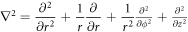

Wave propagation has three degrees of freedom in 3-dimensional Euclidean space, however moving towards fractional-dimensional space, extra degrees of freedom on each dimension in terms of α is achieved. The physical disorder of the general system is captured in terms of α1,α2 and α3. Fractional-dimensional space enables us to further regulate the degrees-of-freedom of the many physical processes within the dimensions of a space, allowing us to describe complicated phenomena. The Laplacian ∇2 D in cylindrical coordinates in a fractional-dimensional space is defined as below [9, 10]:
where α1, α2 and α3 represent the space fractional parameters in respective degree. For mathematical tractability, we make substitution in U0(r, z) = V0(r, z)eikz along with the ∇2 D in equation (1) to obtain the following:

Next, we derive the paraxial wave equation for D-dimension fractional space by applying the paraxial approximation to (4), which results as follows:

Substituting the value of α1 = α2 = α3 = 1 reduces the above equation back to equation (2). We aim to find a generalized Gaussian solution to the space-fractional model by assigning a generalized Gaussian solution as below:

given that, A(z) represents the complex amplitude and p(z) represents the parameter of propagation. Substituting the above solution in equation (5), provides the amplitude of the propagating optical beam at a given distance of z from the transmitter, in space-fractional dimension as:

By setting the values of α1 = α2 = α3 = 1, equation (7) is reduced to non-fractional Gaussian beam wave solution [11]. The Gaussian beam can be express in term of input parameters, including curvature parameter (Θ0) and Fresnel Ratio (Λ0) at the receiver as represented below:

Similarly, the beam characteristics can be express as output parameter at the receiver as:

We set α1 = α2 = 1 to explore the impacts of air turbulence on a space-fractional Gaussian beam along the propagating z-axis. The value of α3 will be varied to see how well it captures the optical beam diffraction due to atmospheric turbulence.
After all the required substitutions in equation (7), the expression for optical beam intensity in term of D-dimensional parameter is achieved as:

given that, WD is the optical beam spreading due to diffraction by turbulence in atmosphere expressed in fractional parameter D. WD is written in terms of α3 as:

where is the complex fractional part. In equation (11), the parameter A is a function of α3, which quantify the intensity of atmospheric turbulence. When α3 = 1, both equations (10) and (11) are reduced down to non-fractional expressions of intensity and beam spot size in free space respectively [11]. For complete theoretical derivation of space fractional paraxial wave equation, a reader can refer to [12].
![$A=1-{\left[z-\tfrac{i({\alpha }_{3}-1)}{2k}\right]}^{\left(\tfrac{{\alpha }_{3}-1}{2}\right)}$](https://content.cld.iop.org/journals/2399-6528/7/1/015002/revision2/jpcoacb1efieqn2.gif)
3. Results and discussion
3.1. Effects of varying α3 on Gaussian beam
To evaluate the characteristics of Gaussian beam propagation in D-dimension fractional model, the FSO link with an operating wavelength measuring 633 nm is selected for a distance of 1200 m. The initial values of the transmitter are set to W0 = 3 cm and F0 = 500 m. The optical link scenario taken into consideration for the proposed model's numerical analysis is shown in figure 1. The Gaussian beam launched at z = 0 m, radiates via the free space before coming to a point called the beam waist, which has the smallest spot size radius and is located shortly before the geometric focus. The beam spot size varies continually due to the effects of refraction and diffraction, once it passes the waist region.

Figure 1. The scheme of propagating optical beam used for this study. The transceivers are kept at a distance of 1200 m from each other, with fixed radius of curvature of F0 = 500 m.
Download figure:
Standard image High-resolution imageWe examine the space-fractional model for propagating Gaussian beam for varying the value of α3 along the propagation path. The results are shown in figure 2, where it can be seen that the spot size of the beam is directly affected by α3. The propagating beam spreads out as the value of α3 reduces. For α3 = 1, the optical Gaussian beam spot size is 4.28 cm, same as the free space spot size. For α3 = 0.7, the beam spreading increases with a spot size of 21.97 cm. This shows the ability of α3 to capture the beam spreading of propagating Gaussian beam.

Figure 2. The spreading of Gaussian beam for altering the α3 values along the path of propagation. Initial beam parameter were set to W0 = 3 cm, at z = 0 m.
Download figure:
Standard image High-resolution image3.2. D-dimensional model for atmospheric turbulence
The existing Kolmogorov turbulence model was proposed for isotropic and sub-inertial range of atmosphere. The Kolmogorov turbulence spectrum model is expressed as follows:

where Cn 2 is the refractive index structure parameter and k is the wave number. The value of Cn 2 is assumed to be constant for horizontal links. The typical values for Cn 2 ranges form strong 10−13 to weak 10−16 atmospheric fluctuations [13, 14]. These atmospheric fluctuations are a result of variations in temperature and pressure, quantified using the Rytov variance, and are represented by:

given L is the distance of propagation between transceivers. The long-term optical beam spot size based upon Rytov approximation, for weak and strong turbulence is mentioned as follows [15]:


where σR is the Rytov variance, W is the free space beam spreading at receiving end and Λ = 2L/kW2.
The measured distribution of space is now defined as D = α1 + α2 + α3, where each α1, α2 and α3 act independently on a single coordinate in the D-dimensional fractional space. As previously stated, the variation in the beam spreading of optical signal along the propagation z-axis is what we are interested in for this study, thus we set α1 = α2 = 1, and α3 is variable.
The results of long-term beam spreading (WD ) for D-dimensional parameter is plotted in figure 3, in comparison to the beam spot size (WLT ) for all levels of atmospheric turbulence including weak and strong fluctuations. The plot shows that WD (11) can capture all levels of fluctuations, as results shows a good agreement with weak (14), as well as strong (15) fluctuation models.

Figure 3. Results of Gaussian beam spreading for weak and strong fluctuation models, in contrast with fractional parameter D. The beam spreading under weak fluctuation conditions verses parameter D is shown in the magnified inset view.
Download figure:
Standard image High-resolution imageThe mapping between the space-fractional parameter D and the refractive index structure parameter Cn 2 is shown in figure 4, which is obtained by using the proposed model and the existing model for weak and strong fluctuations respectively. For a fixed link distance,the value of Cn 2 is assumed constant, and the optical beam spreading (WLT ) is calculated using equations (14) or (15) depending upon the turbulence strength. Now the same value of optical beam spreading is calculated using the space-fractional model (WD ) by varying the value of parameter D in equation (11), to achieve the same amount of beam spreading for the same link length. Once the beam spreading WLT and WD are equal, the value of space-fractional parameter D and Cn 2 can be mapped, as the same amount of optical beam divergence is achieved using both models. For example, the optical beam spreading of received signal is 7.28 cm for atmospheric turbulence strength of , whereas the same amount of beam spreading is achieved using the fractional-space model for D = 2.9. Thus, it can be concluded that the atmospheric turbulence strength can be expressed in terms of fractional parameter D. The plot shows how well the mapping is achieved, leading to a single robust parameter D, capable of expressing the strong and weak atmospheric fluctuations at the same time. For weak turbulence the D-dimensional range varies from 2.991 < D < 3 in contrast to 2.668 < D < 2.99 for strong turbulence.
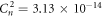

Figure 4. For range of fluctuation levels, the variation in Cn 2 is plotted against the corresponding values of D.
Download figure:
Standard image High-resolution imageThe intensity of the received Gaussian signal is directly impacted by the long-term beam spreading. Intensity profiles for various fractional-dimension parameter D are presented in figure 5, which demonstrates the increasing amount of beam spreading, from D = 3 to D = 2.7.

Figure 5. Illustrating the intensity profile for Gaussian beam propagation in z-axis for various given values of D as: (a) 2.7, (b) 2.8, (c) 2.9 and (d) 3.
Download figure:
Standard image High-resolution imageThe Kolmogorov spectrum is applicable for the sub-inertial range, where it considers the inner scale of zero and an outer scale of infinity. The space-fractional model has been able to capture the beam divergence of optical beam in terms of fractional parameter D, therefore theoretically, it can be concluded that it will be able to capture the beam spreading of the models, considering inner scale as nonzero and a finite outer scale. This can be an extension of the present work.
The proposed space-fractional beam propagation model is unique in nature compared to the existing models for average intensity and optical beam spreading. In comparison to the optical beam intensity models based upon the convolutional property [16], the space-fractional model is distinctive as it expresses the amount of atmospheric turbulence that is experienced by the propagating signal in terms of new mathematical parameter D. Generally speaking, the existing models have their own advantages but are limited to specific atmospheric turbulence conditions, as there are separate model for weak and strong fluctuations respectively, whereas, the space-fractional model is capable of expressing the average intensity and beam spreading in a single fractional parameter D, for all levels of atmospheric fluctuations. This distinguishing characteristic makes the space-fractional model stand out among the existing models.
3.3. Analysis of wavelength dependence
The space-fractional model is analysed for varying the optical wavelength to study the behavior of the model. The input wavelengths of 633 nm, 785 nm and 850 nm were selected and input beam parameter was set to W0 = 3.3 cm and rest of the parameters were kept the same as mentioned in section 3.1. Figure 6 show the plots of WD (11) for varying wavelengths against the D-dimensional parameter along with the corresponding beam spreading value using the Kolmogorov fluctuation models (14), (15), that are depended on Cn 2 and distance. It can be seen that the beam spreading for all wavelengths remains the same from D = 3 to D = 2.85, which shows that the space fractional model is wavelength independent as all the wavelengths have almost the same beam spreading for weak to moderate atmospheric fluctuations. However, for lower values of fractional parameter D, corresponding to increased atmospheric turbulence, the model behaves as wavelength dependent. It can be observed that for values of D < 2.85 the value of WD increases the most for 633 nm compared to 785 nm and 850 nm wavelengths. This shows that higher wavelengths are more resilient to atmospheric turbulence, therefore they can perform better.

Figure 6. The plot for Gaussian beam spreading for wavelengths of 633 nm, 785 nm and 850 nm, for weak and strong fluctuation models, in contrast with fractional parameter D.
Download figure:
Standard image High-resolution image3.4. Link optimization using space-fractional model
The atmospheric conditions can effect the performance of FSO links, therefore it is necessary to operate the link at optimized parameters, so as to ensure the link availability. To optimise the FSO link performance, numerous studies haven been carried out in past, to reduce the atmospheric turbulence effect [17–19]. The optimization of FSO link has been carried out based upon the statistical model [20], for adverse weather condition like fog and strong fluctuations due to high various in temperature. The most crucial optimization parameter in the FSO system for minimizing the effects of turbulence is its optimal beam width size. Keeping this in view, we proposed our analytical D-dimension fractional model as an optimization problem, to adjust the beam width by optimizing the input beam parameters according to the turbulence levels of atmosphere, for achieving steady beam width at receiver.
The space-fractional model minimizes the difference between β, the required spot size at receiving end, and WD (11), the beam spreading expressed in term of parameter D for various turbulent levels.
The variable parameters are the input spot size (W0) and the radius of curvature (F0). The minimization function is written as [12]:

To solve this optimization problem, we used the Matlab optimization toolbox to achieve optimum set of values of input beam parameters, against a constant value of β, for different levels of atmospheric fluctuations.
For the optimization purpose, the value of β was set to 4.28 cm, whereas, the variable parameters including the initial spot size and the radius of curvature, whose ranges were defined as 1 cm <W0 < 3 cm and 470 m <F0 < 580 m respectively. Rest of the parameters were kept same as mentioned in sections 3.1. The results of this optimization are summarized in table 1. We can see random set of optimum input parameters for different values of D, due to the nonlinear nature of the problem.
Table 1. Matlab optimization results showing random set of values for input beam parameters against constant spot size (β = 4.28 cm) at transmitter placed at z = 0 m.
| Cn 2 (m−2/3) | D | W0(cm) | F0(m) |
|---|---|---|---|
| 0 | 3 | 3 | 500 |
| 1.00 × 10⁻¹⁵ | 2.998 | 2.7 | 474 |
| 2.03 × 10⁻¹⁴ | 2.95 | 2 | 478 |
| 3.13 × 10⁻¹⁴ | 2.9 | 2.2 | 548 |
| 4.38 × 10⁻¹⁴ | 2.85 | 2.1 | 575 |
| 5.93 × 10⁻¹⁴ | 2.8 | 1.5 | 500 |
| 7.76 × 10⁻¹⁴ | 2.75 | 1.7 | 549 |
| 9.23 × 10⁻¹⁴ | 2.7 | 1.8 | 570 |
Here we propose an intelligent FSO communication system architecture that can adjust its input beam parameters by sensing the level of atmospheric turbulence, to ensure link reliability by providing constant optical beam spot size at receiver, under different fluctuation levels. Figure 7 display the link design based on the D-dimension fractional model .The transmitter and receiver are equipped with scintillometers that will sense the real-time atmospheric turbulence, expressed as Cn 2, which can be translated through fractional-dimension parameter D. This value of D will act as input to the optimization algorithm that will provide accurate values of input parameter, maintaining constant beam spot size at receiver end irrespective of level of turbulence. This FSO link design can have advantage over existing hybrid FSO/RF models in terms of cost and complexity.

Figure 7. Proposed FSO link design capable of optimizing the input beam parameters in real-time for all levels of atmospheric turbulence, to provide fixed optical beam spot size at receiving end.
Download figure:
Standard image High-resolution image
4. Conclusion
This paper presents an analytical D-dimension fractional model for Gaussian beam propagation through atmospheric turbulence conditions, based on the fractional-dimension approach. The results of the D-dimension fractional model were compared to the existing turbulence models derived from the theory of Kolmogorov and Rytov, for varying atmospheric fluctuations. It showed that the D-dimension fractional model agrees well with the existing ones, as it was able to capture the atmospheric turbulence for all levels of fluctuations, in the range of 2 < D ≤ 3. This leads to one-to-one mapping of the Cn 2 with the dimensional parameter D, for expressing the turbulence of atmosphere in reduced dimensions. The commonly reported Cn 2 lie within the range of 10−13 (strong) to 10−16 (weak) fluctuations, whereas, in fractional-dimension scale, these fluctuations can be expressed as D = 2.668 and D = 2.999, strong and weak fluctuations, respectively. However, the most suitable scenario of free space beam radiation with no turbulence can be expressed as D = 3. The proposed model appears as more generalised with the ability to capture all the turbulence fluctuations within a single parameter D. Moreover, we proposed an optimization based problem with the objective of constant beam spreading at receiving end for varying turbulence conditions, with variable input parameters of initial beam spot size (W0) and radius of curvature (F0). Later, based upon a practical example, we proposed a self-sustainable FSO link architecture to efficiently minimize the weak and strong fluctuations based upon the D-dimension fractional parameter.
The fractional-dimension approach proves to be useful and powerful tool, in expressing the physical behavior of complex mediums such as atmosphere. We can further extend this technique to model the propagation of electromagnetic wave through mediums like oceans, to study the oceanic turbulence [21]. The D-dimensional approach can also be used to study the behavior of optical beam propagating through semi-conductor waveguides, comprising of novel materials [22].
Acknowledgments
The authors would like to thank 'Information Technology University of the Punjab, Lahore, Pakistan' for the support provided to complete this work.
Data availability statement
The data that support the findings of this study are available upon reasonable request from the authors.