

Abstract
The focus of this study is to understand the physical phenomenon of the liquid-based electroactive polymer (EAP) actuator known as the Hydraulically Amplified Self-Healing Electrostatic (HASEL) actuator. Specifically, this study provides data in several areas, including the deformation of the film material, the dynamics of the dielectric liquid, and the electrical conditions within the actuator body. A two-dimensional model was developed in the finite element software, COMSOL Multiphysics, to create a generalized physics-based framework that describes the actuation mechanism. Much of the predictive data agreed well with the experimental data, such as the electrode pull-in occurring at ∼4.5 kV and the displacement-voltage behavior. More importantly, the model also predicts basic fluid dynamic data, such as velocity (which reached a maximum of 0.7 m s−1), the pressure of the fluid within the enclosed film, and the motion of the fluid, which have not been found in previous models. The model also predicts phenomenon seen in experimentation, such as fluid pockets under the electrodes and the interesting displacement-voltage behavior. Everything considered, the model connects the electrical, mechanical, and fluid systems, thus providing more detail about the dynamics of the actuator system and facilitating a shift in the current approach to modeling and designing these actuators.
Export citation and abstract BibTeX RIS

Original content from this work may be used under the terms of the Creative Commons Attribution 4.0 licence. Any further distribution of this work must maintain attribution to the author(s) and the title of the work, journal citation and DOI.
1. Introduction
The crux of a robotic system is the actuation mechanism. For current robots and robotic systems, motors, pneumatic or hydraulic pistons, and other mechanisms are used for actuation; however, these systems have some fundamental weaknesses. Often these actuator mechanisms are bulky, heavy, and rigid, which can lead to problems such as low dexterity and limited usage [1]. However, with the emergence of soft robotic actuation systems, several restrictions of traditional robotic actuation systems can be mitigated. Soft robotic actuation systems are compliant, lightweight, and can be made in a variety of sizes and shapes, which allows for a more varied usage [1, 2]. Also, due to their flexibility and light weight, these soft mechanisms can be used closely with and even mimic biological systems, such as grippers, artificial muscles, and manipulators [3–5].
Electroactive polymer (EAP) actuators are the focus of this study. This type of actuator exhibits deformation when stimulated by an electric field [3]. This study specifically examines the Hydraulically Amplified Self-Healing Electrostatic (HASEL) actuator, which is a novel liquid-based EAP actuator introduced by Keplinger and associates [4, 5]. This device displays many advantageous characteristics: high actuation rates, high strain rates, healing of the dielectric medium at the time of dielectric breakdown, low-cost fabrication, and more [6]. Due to these properties, this actuator has the potential to work in robotic systems, as a low-cost, flexible, and lightweight alternative [4, 5, 7]. However, this actuator is based upon a novel mechanism and further study into the actuator mechanism is essential. This study utilizes finite element modeling techniques to understand the physical characteristics of a typical HASEL actuator.
The HASEL actuator has a fairly complex actuation system because it utilizes two actuation mechanisms from traditional actuation physics: electrostatic actuation and hydraulic actuation [4, 5, 7]. Electrostatic actuation is commonly used for micro-electro-mechanical systems (MEMS), where micro-sized components are driven by the application of a voltage potential [8]. Hydraulic actuation is commonly utilized in larger systems, such as automated industrial systems and large robots, due to the large output capacity and robust design [9]. The HASEL actuator combines these actuation systems to create a scalable and compliant, actuator with large deformation output. The finite element software, COMSOL Multiphysics, is a software tool that can analyze the complex actuation mechanism of the HASEL actuator. Fundamentally this study seeks to describe an alternative to the current state of modeling HASEL actuators, in the hopes of providing more detail on the physics of the actuator system. Thus, the main objective of this study is to use COMSOL Multiphysics to examine the complex physics of the actuator and provide an underlying principle for the HASEL system.
2. Background
2.1. The HASEL actuator
To understand the HASEL actuator, the physical structure must first be described. The typical structure of EAP actuators and liquid-based EAP actuators is generally simple. In the case of the HASEL actuator, it is made from three components: a liquid dielectric, a thin compliant film, and lightweight conductive electrodes. First, the thin, compliant polymer film is shaped to create a shell that encapsulates the dielectric fluid [4, 5, 7]. After the fluid is injected into the film, the compliant electrodes sandwich the fluid-filled pouch (figure 1).

Figure 1. (Left) 3D model of a HASEL actuator with the compliant electrode, the clear film, and liquid dielectric. (Right) A HASEL actuator from experimentation, the compliant electrode is created from carbon tape, the film material here is Low-Density Polyethylene (LDPE), and the liquid dielectric is mineral oil.
Download figure:
Standard image High-resolution image2.2. The proposed actuation mechanism of HASEL
To obtain a sense of how the model is shaped, a more in-depth background on the two actuation mechanisms is needed. The electrostatic actuation mechanism is based on the use of the Maxwell Stress tensor, and further the electrostatic forces, to cause a deformation in a compliant material [4, 5, 10–14]. In the case of a typical dielectric actuator, a dielectric material is placed between two electrodes; the electrodes are charged with a voltage and the charge of the dielectric aligns with the electric field that is generated [14–17]. The change in the alignment of the dielectric causes a change in the compliant material [3]. In the case of the HASEL actuator, when the electrodes are charged and a critical voltage is reached (typically ∼4 to 5 kV) the compliant electrodes and the film that encapsulates the fluid, collapse toward each other from one end of the electrode to the other [10, 11, 13, 18].
Considering the hydraulic mechanism, when the electrodes buckle at the critical voltage and close together, the majority of the fluid is pushed into the area of the actuator not covered by activated electrodes (figure 2) [19].
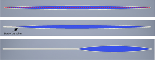
Figure 2. A cross-sectional view of the actuator during various actuation states. (Top) The state of the actuator when no voltage is applied. (Middle) The state of the actuator when the critical voltage has been reached and the actuator begins to 'zip' or pull-in. (Bottom) The state of the liquid-based actuator fully 'zipped'; thus, the electrodes have fully pulled in toward each other. More information can be found from [20].
Download figure:
Standard image High-resolution image3. Modeling
3.1. Previous modeling work
Previous efforts have gone into modeling the physics of the HASEL actuator, using different approaches than the work presented for this study. Kellaris et al describes an analytical model that uses the free energy of the system as the focus for describing the behavior of the actuator [7]. Wang et al considers an analytical model as well; however, this model is designed for high strain Peano-HASEL actuators [15]. The model developed by Wang et al does not consider the material mechanics, the electric field across the entire actuator, and some end boundary conditions [15]. The models devised by Kellaris and Wang both parameterize the geometry of the analysis region about a central angle, denoted as  By using this method, the strain and force behavior is described. Rothemund et al proposed a dynamic model of liquid-based HASEL actuators by considering experimental work, scaling analysis, and fitting parameters [16]. The dynamic model was built using dimensional analysis and Lagrange's second-order equations; the model determines how different factors affect the actuation speed [16]. Manion et. al built a finite element model in ANSYS that primarily focused on characterizing a custom polymer shell [17]. The finite element model considers a circular geometry and applies Neo-Hookean mechanics to the material. To approximate the effect of the 'zipping' on the fluid, the model uses an internal volume approximation and does not consider the internal pressure gradients.
The current modeling approach in this study takes a broader view and considers how the material, geometry, fluid, applied voltage, and other parameters affect the system as a whole dynamically. The use of COMSOL Multiphysics allows the analytical physics to be further tied together, allowing for this broader scope into the deformation, fluid movement, electrostatics, etc. However, the most important factor of this model is the presentation of the dynamic performance, including the fluid dynamics, fluid properties, and the relationship of the fluid mechanics, solid mechanics, and the electrostatics physics. The dynamic performance, specifically in relation to the fluid has not been found in other literature [21]. Additionally, this model opens up the opportunity for larger model customization; the model parameters, such as the materials and the testing conditions, can be easily changed to better estimate the behavior of the actuator when changes are made to the system. The following table further describes equipollent models that focus on liquid-based EAP actuators or models that influenced their design (table 1).
Table 1. Comparison of Previous Models to the Current Model Study.
| Article | Model Type | Authors (Year) | Contribution |
|---|---|---|---|
| An analytical model for the design of Peano-HASEL actuators with drastically improved performance | Analytical Model [7] | N. Kellaris et al (2019) | Describes the quasi-static behavior for different geometries and materials. |
| High-Strain Peano-HASEL Actuators | Analytical Model [15] | Wang et al (2020) | Describes the quasi-static behavior for high strain Peano-HASEL actuators. |
| Zipping dielectric elastomer actuators: Characterization, design and modeling | Finite Element Model [11] | Maffli et al (2013) | Describes the electrode pull-in behavior of compliant film and electrode materials. |
| Optimum design of an electrostatic zipper | Analytical Model [10] | Brenner et al (2004) | Describes a numerical method to predict the optimal conditions for compliant electrode pull-in. |
| Dynamics of electrohydraulic soft actuators | Analytical Model [16] | Rothemund et al (2020) | Provides predictive data on actuation speed based on the influence of distinct parameters. |
| Modeling and Evaluation of Additive Manufactured HASEL Actuators | Finite Element Model [17] | Manion et al (2018) | Provides actuation strain data on the additively manufactured film material used for custom HASEL actuators. |
| Current Model Study | Finite Element Model | This work | Simulates the electric field and provides predictive data on film deformation; the fluid motion and general fluid dynamic properties; and preliminary data on the output force-displacement relationship. |
3.2. The COMSOL multiphysics model
As mentioned previously, this modeling study utilizes COMSOL Multiphysics, a finite element software. The underlying physics can be described in three major components which are then subsequently coupled. The three main components of the model are based upon solid mechanics, electrostatics, and fluid dynamics.
3.2.1. The model set-up
This section describes the foundational set-up for this finite element model; this includes the description of the geometry, domain definitions, and some constraints and conditions for the model. The current model is modeled in two space dimensions, the analysis is conducted along the cross-section along the x-y plane. In this model the electrode is not given a defined domain due to a couple of factors. First, in comparing the polymer film and the electrodes used for experimentation, it was found that the stiffness of the electrode must be much smaller than that of the polymer film to have good actuation. Thus, the system is more dependent on the fluid and the polymer film. Also, a minor point this study seeks to observe is the relationship between the solid and liquid dielectric mediums from a materials standpoint. However, the electrodes are defined as boundary conditions, thus still providing an effect on the actuator system.
Additional constraints and conditions on the system include the left-most edge of the solid film domain is fixed to ensure the structural problem is well-posed. This treats the edge as a datum point for the deformation to be measured. It is important to note that the response of the actuator is fast, and a great deal of deformation occurs within that time frame, therefore in order to capture the motion of the actuator system, this model considers a time-dependent study. In other words, this work studies the transient deformation of the HASEL actuator in order to investigate the initial electrode pull-in.
3.2.2. The solid mechanics
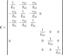
Firstly, the solid mechanics is applied to the film, wherein the film is classified an orthotropic material according to the commercial materials used in experimentation. This allows for more customization when modeling the film material. Currently, the material variables relevant to the model are the elastic moduli (E), shear moduli (G), the Poisson's Ratio ( ), and the density (
 ). The material model is described by equation (1), where
  is the strain vector,
  is the stress vector, and
C
is the compliance matrix. Further, the equation of motion for the study is described by equation (2), where
u
is the displacement field, P is the Piola-Kirchhoff stress, and
F
V is the volume force vector.
is the stress vector, and
C
is the compliance matrix. Further, the equation of motion for the study is described by equation (2), where
u
is the displacement field, P is the Piola-Kirchhoff stress, and
F
V is the volume force vector.


Considering several factors such as the material properties, the interaction of different materials, and the expectation of extreme deformations, the deformation is described using a finite strain and material frame formulation.
3.2.3. The electrostatics and the electromechanical coupling
The electrostatics has a major effect on the solid mechanics physics and the model as a whole. Within the electrostatics physics, the dielectric liquid and the film material are described as the regions of interest because the film and the liquid act as the deformable dielectric medium. To begin, the scalar electric potential is defined about the x-axis of the 2D actuator profile. The initial applied voltage is represented through the electrode boundary, the top-left boundary of the actuator geometry and the midplane voltage is defined as a voltage boundary along the x-axis of the system (figure 3). Thus, the electrode boundary voltage is defined at the input ramped voltage, V1, and the x-axis boundary voltage condition is defined as  For this study, the dielectric material is linear, thus the relationship between the electric field and the dielectric constant (equation (3a
)) can be described by Gauss's Law and the relationship between the electric field and the voltage potential can be described by Faraday's law (equation (3b
)).
For this study, the dielectric material is linear, thus the relationship between the electric field and the dielectric constant (equation (3a
)) can be described by Gauss's Law and the relationship between the electric field and the voltage potential can be described by Faraday's law (equation (3b
)).


Figure 3. (Left) The boundary highlighted in blue is defined for the applied voltage and the surface traction for the electromechanical coupling. (Right) The boundary highlighted in blue is defined for the applied voltage symmetry constraint.
Download figure:
Standard image High-resolution imageBecause the electrode boundary and the dielectric domain are defined by electrostatics physics, the Maxwell stress can be defined along the electrode boundary. Therefore, to couple the solid mechanics and the electrostatics, the Maxwell stress (only accounting for the x and y components) is applied as a surface traction along the electrode boundary (figure 3). The Maxwell stress tensor is derived beginning with the Lorenz force equation,  It is at this point that the Maxwell equation is modified from its typical derivation. Here the relationship between
  (the total volume charge density), E, and D is of import; in dielectric materials the charges face polarization within the material. Instead of defining the charge distribution as equation (3a
), Gauss's Law is reintroduced to define the electric displacement field (equation (3c
)).
(the total volume charge density), E, and D is of import; in dielectric materials the charges face polarization within the material. Instead of defining the charge distribution as equation (3a
), Gauss's Law is reintroduced to define the electric displacement field (equation (3c
)).

Considering this definition, the Maxwell stress tensor is derived to obtain equation (4a ). This system does not include a magnetic field; thus, the stress tensor can be further reduced to equation (4b ).


Where
D
is the electric displacement field,  is the free charge density,
E
is the electric field,
B
is the magnetic field, V is the voltage potential, is the charge velocity, σij is the stress tensor, ε0 is the vacuum permittivity (8.854 × 10⁻¹² F
is the free charge density,
E
is the electric field,
B
is the magnetic field, V is the voltage potential, is the charge velocity, σij is the stress tensor, ε0 is the vacuum permittivity (8.854 × 10⁻¹² F m−1),
m−1),  is the relative permittivity, δij is Kronecker's delta, and μ0 is the vacuum permeability (1.256 × 10⁻⁶ NA2).
The surface traction (
T
app
) is based on the Maxwell stress and the surface normal of the interface ( ) [equation (5)].

3.2.4. The fluid mechanics and the solid-fluid interface
Lastly, the physics of the fluid is considered. For this model, laminar, incompressible flow [5] using a Newtonian fluid is considered; the Navier–Stokes equation and the continuity equation describes the dynamics of the dielectric fluid within the film pouch as seen in equations (6a ) and (6b ).


Where  is the density of the fluid,
u
is the velocity of the fluid, p is the pressure of the fluid,
is the density of the fluid,
u
is the velocity of the fluid, p is the pressure of the fluid,  is the dynamic viscosity of the fluid,
I
is the identity tensor, and
F
is the externally applied forces.
is the dynamic viscosity of the fluid,
I
is the identity tensor, and
F
is the externally applied forces.
Because the major physics components affect each other greatly, the fluid-structure interaction physics module is used to adequately apply all the physics described above to the model. This creates a coupled boundary pair between the solid film geometry and the liquid dielectric, which allows the finite element solver to compute both simultaneously.
The specific parameters given for this model are based on measurements taken in the lab, literature, or experimental conditions used in current in situ experimentation. The thickness of the polymer film and actuator was taken in the laboratory using a digital micrometer. The mechanical properties of the film and fluid properties were found in literature [22–28]. The applied voltage is the variable parameter. The model parameters for the polymer film shell and the parameters for the dielectric fluid are described in tables 2 and 3, respectively. These parameters can be conveniently changed within the model allowing for a wider variety of analyses and results.


3.2.5. The finite element mesh
Due to the large displacement of the fluid, the mesh is an important factor of the model. Due to the coupling of the different physics systems, the mesh generated by COMSOL is based on the established physics systems. By utilizing the physics-based meshing system, the mesh will be more stable as it tracks the changes in the model over time. Taking a closer look at the mesh (figure 4), the film layer consists of a coarse triangular mesh. A triangular mesh simpler for the program to generate and works best for systems with more complex geometries. Also, more elements are generated (compared to a quadrilateral mesh), allowing for more of the physics to operate properly. The coarse mesh option was chosen to decrease computation time.
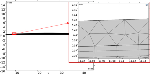
Figure 4. The course triangular film mesh layer generated in COMSOL Multiphysics.
Download figure:
Standard image High-resolution image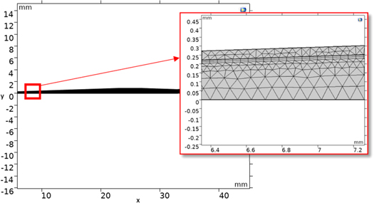
Figure 5. The generated mesh for the model study, magnified for clarity.
Download figure:
Standard image High-resolution imageThe fluid-solid interface is meshed in a particular way because the physics is based on the shared boundary conditions. The structural deformation of the film mesh transfers the deformation to all the shared boundaries of the fluid. Thus, at the interface between the solid film and the liquid dielectric, a quadrilateral mesh is generated (figure 5). This type of mesh is preferable when considering highly deformable regions; the error approximation and number of elements is reduced compared to triangular meshes. Although the entire system is highly compliant the interface between the solid and the fluid is quite important, thus the characteristics of the quadrilateral mesh are favorable [29].
Beyond the mesh of the solid-fluid interface, the fluid mesh is also a triangular mesh. For this actuator type, a significant portion of the liquid dielectric is displaced within the film pocket and the film itself deforms quite quickly. To provide a solution, the mesh must be able to track the deformation of the actuator. To accomplish this, an adaptive mesh refinement solver is applied. COMSOL will solve the physics on the initial mesh as usual, then an error estimation will be made. The error estimation will locate the areas of the mesh that are causing large errors. The program will then re-mesh those areas (creating a finer mesh) and attempt to solve the solution on the newly formed mesh. The error estimation is based on the Euclidean norm (L2 norm) for the voltage. The error estimation is in the form seen in equation (7).

The gradient of the output voltage potential across the electrodes is taken as the indicator variable. This is because this voltage potential across the electrodes drives the physics. The input voltage at the boundary does begin the actuation process but the output voltage potential directly relates to the electric field that is generated throughout the materials; the electric field then relates to Gauss's Law, Faraday's Law, and the Maxwell Stress, which further drives the simulation.
4. Results
The conditions of the model simulation are similar to the conditions used in experimental work within the laboratory. In the experimental work, a fast-ramping condition is applied to the system, wherein a DC voltage is applied from 0 to 10 kV quickly. The model simulates this similar condition, such that the input voltage is ramped from 0 to 10 kV in 0.135 s (supplementary materials-figure 1 (available online at stacks.iop.org/JPCO/6/085007/mmedia)). With this ramping condition, the response time in relation to the deformation, the fluid velocity, the fluid pressure, and more can be determined. From the time the activation voltage is applied and ramped, the actuator is fully 'zipped' by 0.132 s (figure 6). Based on the deformation surface plots, the critical pull-in voltage begins at 4.5 kV (0.06 s) (figures 7 and 8).
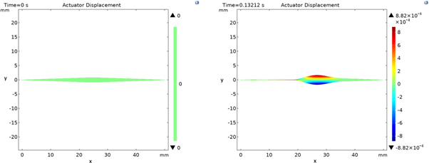
Figure 6. (Left) The actuator model with no applied voltage. (Right) The model with fill electrode pull-in.
Download figure:
Standard image High-resolution image
Figure 7. (Left) The left end point of the actuator model with no applied voltage. (Right) The left end point of the actuator model when the critical voltage is reached (4.5 kV) and the pull-in begins, the material begins to noticeably pull away from its original position (indicated by the outline).
Download figure:
Standard image High-resolution image
Figure 8. (Left) The experimental actuator with no applied voltage. (Right) The experimental actuator beginning to 'zip' at the critical voltage ∼4.5 kV; as the electrodes beginning to zip in the corners (denoted by the arrows).
Download figure:
Standard image High-resolution imageThe resultant area of examination is where the actuator begins to taper back down, this is the point where the maximum displacement takes place. At this location the most motion and largest force output from the actuation will occur; depending on the application of the actuator this point is of particular importance. The displacement in the y-direction has a steady increase, a decrease, followed by a sharp increase (figure 9). When the electrode pull-in occurs, the fluid near the electrodes begins to be displaced; however, the fluid at the midpoint of the actuator is displaced as well but at a slower rate. Figure 10 shows this disparity in the location of fluid at 0.08 s.

Figure 9. (Left) The red point denoting the point of maximum displacement. (Right) The y-displacement of the HASEL actuator model. Maximum displacement occurs at 0.879 mm.
Download figure:
Standard image High-resolution image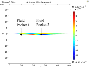
Figure 10. The deformation of the actuator at 0.08 s, at this point the formation of two distinct fluid pockets is apparent.
Download figure:
Standard image High-resolution imageThe fluid dynamics results further explain the actuator behavior and support the phenomena seen from the displacement results. Examining the fluid velocity data (see Supplemental Materials-figure 2) indicates that there are two regimes. The first regime shows the velocity of the fluid being displaced by the pull-in of the electrodes. The second regime shows the slower, but significant movement of the larger fluid pocket at the midpoint of the actuator. The electrodes close further, and the velocity of the first fluid pocket increases but the velocity of the second fluid pocket begins to stagnate, creating more distinct fluid pockets. As the 'zipping' continues, the speed of the fluid in the first pocket increases and the speed in the second pocket decreases. However, the two distinct pockets still remain, leaving a section of the actuator with a dip or 'bottleneck' in the material and the fluid. This dip causes the sharp decrease seen in the deformation results. Finally, the electrodes fully close, and one large fluid pocket remains with the film and fluid at the maximum deformation as seen in the deformation results.
The fluid pressure results show the maximum pressure in the fluid begins where the electrode pull-in begins (supplemental materials - figure 3). This pressure steadily increases as the electrodes 'zip' closed. Once the actuator electrodes are fully pulled-in there is a small pocket of fluid under the electrodes, causing high-pressure points on either side of the small pocket. Also, a small thin layer of fluid remains between the film. These results predict that liquid-based EAPs do not fully actuate due to the fact that not all of the fluid is displaced. Depending on the actuator application this could be beneficial. By having a small film layer under the electrodes, it is possible that the direction of the fluid can be controlled with the manipulation of the electrode design.
The model provides basic information of the force-displacement relationship. To acquire these results, a boundary load of 1 g m−2 was placed along the top right boundary to act as load that the actuator pushes against (figure 11). The response time results show that the actuator performs similarly to an unload actuator with the maximum displacement reached in 0.139 s. The results also determined that the overall displacement decreased and showed a similar displacement curve until a critical point is reached, then actuator begins to compress rapidly (figure 12). The force-displacement curve shows as the force is applied; the actuator reacts with a rapid increase in the displacement until the maximum pressure is reached at 1334.3 N m−2. The displacement is then followed by a sharp decrease, and it reaches almost zero, then actuator seemingly 'reactivates', and the displacement increases again (figure 12).

Figure 11. The boundary highlighted in blue is the application of the boundary load.
Download figure:
Standard image High-resolution image
Figure 12. (Left) The y-component of the displacement field when a load is applied along the boundary of the actuator. (Right) The force per unit area-displacement curve under the loading conditions.
Download figure:
Standard image High-resolution image5. Discussion
The following section considers the findings from this study. Considering the overall results, the actuator fully displaces the fluid in 0.132 s which can be considered a quick response time. These results correlate with data found in the literature and experimental work [4, 5]. It is important to note that the response time is based on the time in which the voltage potential is applied. For this study the voltage was applied very quickly, subsequently causing a quick actuation response in turn. In addition to the fast response time, the model results describe the maximum displacement as 0.879 mm. The model results are compared to the experimental results, the experimental displacement is measured with the use of a 1-dimensional laser displacement sensor (Micro-Epsilon optoNCDT 1400 series model). The model result falls short of the preliminary experimental results of a maximum deformation range from ∼1.5 mm to 3.3 mm. However, the experimental results do display a similar displacement behavior that is seen in the displacement prediction of the model. There is little to no actuation, then a dip after the visible activation point (around 4.5 to 5 kV, see figures 9 and 13), and finally a rapid increase in the displacement of the actuator. Although the maximum displacement output of model does not perfectly align with the maximum displacement output of the experimental data, the model is capturing how the fluid moves within the actuator packet.

Figure 13. The experimental displacement of a single HASEL actuator unit ranging from activation voltages 1 kV to 10 kV.
Download figure:
Standard image High-resolution imageThe model results show that the critical voltage is at 4.5 kV (0.06 s). This result agrees well with experimental results, in which the critical pull-in voltage is around ∼4.5 to 5 kV (figure 9 and supplemental materials-figure 4). Beyond the visual of the electrode pull-in, the displacement data taken in experimentation describes the actuator displacement at each activation voltage (supplemental materials-figure 4). There is very little activation at 4 kV, but there is a substantial jump in the displacement at an activation voltage of 5 kV. Thus, within the range of ∼4.5 kV to 5 kV, the critical pull-in stage is reached.
Upon further examining the deformation results, the increase and sharp decrease in the data describes the creation of the two fluid pockets, this is most likely due to a combination of the initial pull-in of the electrodes and the fact that the majority of the fluid is at the midpoint of the actuator. Once the fluid under the electrode begins to move due to the electrode pull-in, the fluid that settles at the midpoint also begins moving at a slower rate. The creation of two fluid pockets could also be due to the viscosity of the fluid used for this model.
Closely examining the fluid velocity results, it is shown that the second fluid pocket does in fact move at a slower velocity than the first velocity pocket. This in turn creates the 'bottleneck' or dip in the deformation of the film. As mentioned previously, this dip in the film between the two pockets creates a decrease in the deformation result. The fluid velocity results directly support the deformation results and interpretation. There is a negative fluid velocity in front of the large fluid pocket (supplemental materials-figure 2). This negative velocity is residual fluid displacement from the second fluid pocket. As the second fluid pocket moves closer to the right end of the actuator, the velocity decreases as it is stopped by the film material. Further, some of the fluid moves backward and joins the larger, final fluid pocket. This phenomenon is further validated by the experimental results. Again, looking at the data highlighted in figures 9 and 13, after the critical pull-in voltage is reached there is a decrease in the displacement (at about 6 kV) and then a rapid increase in the displacement.
The fluid pressure results show that the majority of the pressure on the fluid is concentrated under the electrodes, where the force is being applied. However, there is a very small fluid pocket that forms once the electrodes are fully closed (supplemental materials-figure 3). The formation of this fluid pocket is most likely caused by the geometry of the actuator and the material of the actuator. The actuator is made of compliant film and the geometry is oriented in such a way that the end condition of the actuator resembles a flexible beam that is angled, with an end loading condition (supplemental materials - figure 5). As the flexible films close toward each other, there are points where the film buckles, such that the thickness between the electrodes is smaller at the end point of the film than in the middle (supplemental materials - figure 5). The end points of the films are drawn toward each other and close fully, but the viscous fluid is trapped under the area where the film buckled, creating a small fluid pocket. There is also an increase of the fluid pressure around this small fluid pocket caused by the pocket itself. This type of uneven electrode pull-in is seen in experimentation as well (figure 14).
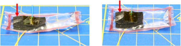
Figure 14. A fully zipped actuator from experimentation. The arrows indicate areas where film and electrode material buckle and some of the liquid dielectric becomes trapped, creating small fluid pockets under the electrode.
Download figure:
Standard image High-resolution imageThe results for loaded actuator condition show that there is very little change in the response time, which indicates that these actuators could work well for various robotic applications, where a rapid response time is needed. However, the overall displacement of the actuator significantly decreases compared to an unloaded actuator. This result is consistent based on basic physics principles. This model predicts a sharp decrease in the displacement once a critical force is reached. At this critical point the actuator begins to compress due to the loading and almost reaches zero displacement. Then the actuator seemingly 'reactivates', and the force-displacement curve sharply increases again. However, looking at the overall y-displacement, it is clear that the actuator does not actually reactivate. This phenomenon is caused by a combination of the loading condition and the electromechanical relationship. From the unloaded condition it can be seen that, as the electrodes pull-in the film deforms and pushes the fluid to the other section of the cavity. However, when the actuator is loaded there is a point where the applied load traction overwhelms the induced Maxwell stress surface traction. The fluid then rushes back and separates the electrodes, causing the sharp decrease in the actuator displacement. However, looking at the force-displacement curve, the displacement rapidly increases once again. Because the applied voltage is still in effect, the molecules of the dielectric medium have maintained the polarized state and the Maxwell stress surface traction is still in effect. The actuator cannot achieve the same state as it previously did (due to the applied loading), but the induced Maxwell stress surface traction slows the rate at which the deformation is decreasing (figure 15). Additional experimental data under a 10 g loading condition, shows similar results to the model (figure 15). Firstly, the experimental results show that the overall displacement of the actuator decreases when under a constant load. Secondly, the response time is also slightly delayed with electrode pull-in beginning at 5 kV (0.067 s) (supplemental materials - figure 6), compared to 4.5 kV (0.06 s) for the unloaded actuator (figure 13). Finally, the experimental actuator displays the same initial displacement curve as seen in the model (figures 12 and 15). The model results indicate overloading in robotic systems can cause failure. Overall, under a loading condition, the model predicts that the actuators will perform.

Figure 15. Experimental displacement of a single HASEL actuator unit with the application of a 10 g mass.
Download figure:
Standard image High-resolution image
6. Conclusion
The main goal of this study was to provide understanding of the HASEL actuator's actuation mechanism. This was achieved through the use of the finite element software COMSOL Multiphysics. By utilizing this physics-based modeling approach, predictions about liquid-based EAP actuator behavior are described. The model was able to provide results about the actuator materials and motion. Firstly, the results predicted the response time and the displacement in relation to the applied voltage for a single actuator unit. This information is important to predict for application purposes. These actuator units can be used in a variety of manners including robotic grippers or artificial muscles; however, the high applied voltage can limit the actuator's use [19]. Using this physics-based model to predict the displacement in relation to the applied voltage can lead to a more effective application of the actuators.
In addition to the response time and displacement results, the model study also predicts the motion of the fluid within the packet. The fluid motion is important because the fluid causes the deformation and acts as the dielectric medium by which the actual activation of the actuator mechanism occurs. By nature, the liquid-based EAP actuators have a seemingly ON/OFF response. However, the results from the model and experimentation indicate that there may be a way to control the actuator response. Beyond application purposes, the use of finite element methods provides an improved prediction and exploration of the interaction of the materials, the materials' reaction to the voltage stimuli, and the dynamics of the actuator.
All in all, this model helps predict the dynamic motion of the actuator, how the applied voltage affects materials, the response time, the motion of the fluid within the film, and other actuator results. This information provides fundamental guidance for optimizing the actuator design and for determining effective applications of this actuator type. The current model can accommodate a variety of changes in the material properties and applied voltage properties, which allows for diversity in the actuator design. However, due to the complexity of this actuator and the wide variety of actuator geometries and materials, future work will focus on refining the model to accommodate a larger variety of customization. Overall, a new methodology for modeling these actuators was presented and the study described the dynamic HASEL actuation mechanism.
Acknowledgments
This work is supported by the NASA's Office of STEM Engagement/NASA Fellowship to A W (OSTEM; Grant Number 80NSSC20K14720). Also, K J K acknowledges the partial financial support from the US National Science Foundation (NSF), Partnerships for International Research and Education (PIRE) Program, Grant No. 1545857. Any opinions, findings and conclusions or recommendations expressed in this material are those of the author(s) and do not necessarily reflect the views of the NSF.
Data availability statement
The data that support the findings of this study are available upon reasonable request from the authors.