
Abstract
We present a new rigid-ion force-field for the alkali metal nitrates that is suitable for simulating solution chemistry, crystallisation and polymorphism. We show that it gives a good representation of the crystal structures, lattice energies, elastic and dielectric properties of these compounds over a wide range of temperatures. Since all the alkali metal nitrates are fitted together using a common model for the nitrate anion, the force-field is also suitable for simulating solid solutions. We use the popular Joung and Cheatham model for the interactions of the alkali metal cations with water and obtain the interaction of the nitrate ion with water by fitting to a hydrate.
Export citation and abstract BibTeX RIS

Original content from this work may be used under the terms of the Creative Commons Attribution 4.0 licence. Any further distribution of this work must maintain attribution to the author(s) and the title of the work, journal citation and DOI.
1. Introduction
Nucleation and crystal growth are fascinating phenomena that require computationally expensive tools to be fully understood [1, 2]. Recent studies have focused on molecular anion systems, particularly carbonates, phosphates and sulphates, due to their biological and industrial relevance [3]. Alkali metal nitrates are made up of a monovalent cation and a simple triangular molecular ion. They show a widely diffused polymorphism which makes them interesting to study [4]. NaNO3 has an extended second-order polymorphic transition and is a model for the isostructural calcite mineral (CaCO3). KNO3 is polymorphic: α-KNO3 takes the aragonite structure; β-KNO3 is trigonal; γ-KNO3 is also trigonal but has no centre of symmetry; high pressure phases also exist. RbNO3 has a rich polymorphism with four phases at ambient pressure. The stable polymorph (phase IV) at room temperature has a complex trigonal structure. The end members; LiNO3 and CsNO3, are monomorphic. All alkali metal nitrates possess high solubility, so simulations are far better able to link to experimental conditions since smaller simulation boxes can be used.
Modelling these systems relies on good quality force-fields, which must be as accurate and consistent as possible without being computationally expensive. It is essential to balance computational cost against the ability of the simulation to reproduce the observed phenomena. A model must be transferable, so that it can be used for all the phases of a given nitrate and, if possible, the same representation of the nitrate anion should be used throughout so that solid solutions can be simulated (the nitrate ion is often kept rigid to simplify calculations, but we shall use a flexible model here). We focus on potassium nitrate because it presents polymorphs similar to those of calcium carbonate. The similarities between those two systems make potassium nitrate a good candidate for a model system to understand calcium carbonate itself. In this paper, we fit a reliable set of force-fields in order to be able to simulate the nucleation and growth of the alkali metal nitrates and use them to help understand the mechanisms of crystallisation.
Several previous force-fields have been developed (e.g. Hammond et al [5] (Li, Rb), Ribeiro et al [6] (Li, Na, K, Cs), Xie et al [7] (Li, Na, K), Ni et al [8] (Li, Na, K), Mort et al [9] (Na, K) and Jayaraman et al [10] (Li, Na, K)). These have been developed for high temperature molten mixtures (Ribeiro, Jayaraman), solutions (Hammond, Xie, Ni), and defect chemistry (Mort) but no force-field has been developed that can be used across all of the alkali metal nitrates and none of them are really suitable for investigating crystallisation. The shortcomings of the various existing force-fields are discussed in detail in the supplementary material (available online at stacks.iop.org/JPCO/6/055011/mmedia). Briefly, Ni, Xie and Mort fail to obtain the correct order for the relative energy of polymorphs in some nitrates; Ribeiro fails to optimise several crystal structures; none of the models (except that of Hammond) predict real values for all the high-symmetry branches of the phonon spectra of the polymorphs to which they were fitted (showing that the true predicted structure must be of lower symmetry than the ones considered). The existing force-fields are adequate for the purposes they were intended for but there is clearly room for improvement. Also, there is no force-field that is suitable for all the alkali metal nitrates, their solution chemistry and their solid state solutions. Before we discuss details of the fitting, we review the structures of the alkali metal nitrates.
1.1. Structures of the alkali metal nitrates
1.1.1. Lithium nitrate
Crystallises in the rhombohedral  group at 290 K with Z = 6, a = 4.692 Å, c = 15.2149 Å [11] (isostructural with calcite). So it will have a Bravais-Friedel-Donnay-Harker morphology showing
 and
and  forms [12].
1.1.2. Sodium nitrate
Crystallises in the rhombohedral  group at 298 K with Z = 6, a = 5.0396 Å and c = 16.829 Å (II-NaNO3) [13] and becomes a high-temperature disordered phase (
 I-NaNO3) at 548.5 K. This polymorph has Z = 3, a = 5.0889 Å and c = 8.868 Å. The nitrate group appears to be static in the low temperature phase but undergoes rotational disorder in the high-temperature phase [14]. Both carbonate and nitrate groups show disordered high temperature phases. Starting from a pure solution it is possible to grow single
  rhombohedral crystals [15] whilst adding Li+ and K+ ions to the solution produces
  crystals [16].
1.1.3. Potassium nitrate
Exists in three different polymorphic forms at atmospheric pressure [17]: I, β-KNO3 rhombohedral  stable at 403 K with a = 5.42 Å and c = 19.41 Å [18]; II, α-KNO3 aragonite
  stable at 299 K; a = 6.2703 Å, b = 5.3935 Å, c = 9.1366 Å [19], III γ-KNO3, rhombohedral,
  ferroelectric, stable at 397 K, with a = 5.43 Å and c = 9.112 Å [20]. On cooling phase III to 383 K it is possible to recover phase II. There is a metastable monoclinic phase (
 -KNO3 [21]) and a high-pressure orthorhombic phase (IV) [22]. Below 305 K KNO3 mostly has the growth forms

 and
and  [4].
[4].
1.1.4. Rubidium and caesium nitrate
Crystallise in a complex trigonal structure (Z = 9; P31, a = 10.55 Å, c = 7.47 Å (RbNO3 at 298 K) [23] and a = 10.902 Å, c = 7.74 Å (CsNO3 at 296 K)) [24].
Standard thermodynamic data is quoted in the literature for some of the polymorphs. Rao and Rao [25] discuss the enthalpies of transformation that are available. They conclude that the most reliable data are when there is agreement between the differential thermal analysis and calorimetric values. There are two examples known: for KNO3 (phase II (Pnma) → phase I ( ));
));  kJ mol−1) and for RbNO3 (phase IV (P31) → phase III (
 ));
));  kJ mol−1). These small differences make reproducing the order of stability of the polymorphs a serious challenge. Figure 1 (below) shows the structures for the four space-groups where all the sites are fully occupied that have been used in the fitting process.

Figure 1. Structures of the phases of the alkali metal nitrates that are used in the fitting. Purple spheres are the alkali metal ions; light blue spheres are the nitrogen atoms; red spheres are the oxygen atoms.
Download figure:
Standard image High-resolution image2. Methodologies
We require a force-field that can describe alkali metal nitrates equally well in solution and as a solid phase. To keep the costs of molecular dynamics simulations down, a rigid ion model with flexible nitrate ions was used. This type of model has proved successful for many molecular ions, in particular the carbonates and sulphates. Full ionic charges (qM = 1) are used for the alkali metal ions. The fitting of charges on the nitrogen and oxygen atoms is discussed below. Buckingham potentials were used for all intermolecular interactions except for those between the alkali metal cations where the Lennard-Jones form was used for consistency with the model of Joung and Cheatham [26], frequently used to study solution chemistry of the alkali halides. The parameters for these interactions are given in table 1.
Table 1. Interactions between alkali metal ions [26] qM = 1.0 for M = Li-Cs where ε and Rmin are defined as the energy and interatomic distance at the minimum, i.e. we use the Lennard-Jones potential in the form ![$V\left(r\right)=\varepsilon \left[{\left(\displaystyle \frac{{R}_{min}}{r}\right)}^{12}-2{\left(\displaystyle \frac{{R}_{min}}{r}\right)}^{6}\right].$](https://content.cld.iop.org/journals/2399-6528/6/5/055011/revision2/jpcoac6e2bieqn21.gif)
| Alkali ions | ε(eV) | Rmin (Å) |
|---|---|---|
| Li-Li | 0.01459 | 1.582 |
| Na-Na | 0.01528 | 2.424 |
| K-K | 0.01860 | 3.186 |
| Rb-Rb | 0.01930 | 3.474 |
| Cs-Cs | 0.00390 | 4.042 |
A force-field developed by Ratieri et al [27] for the carbonate anion was used as a starting point for the nitrate but with the initial partial charges adjusted (using charges from electronic structure calculations as a guide) to give the correct overall charge on the nitrate anion and subsequently fitted to the crystal structures and properties as described below. To describe the interactions within the nitrate group, harmonic interactions were used for the N-O bond and three-body bond-angle potentials used to maintain the preferred angle between the bonds. Further many-body interactions were added (as specified by Raiteri et al) to maintain the planarity of the nitrate anion. Coulomb subtraction was applied within all the nitrate molecules. Examination of the Raman lines demonstrated that the internal interactions of the carbonate group could approximate the internal interactions of the nitrate group. The force-field for the nitrate anion is given in table 2. A tapering cut-off for the short-range intermolecular potentials was applied during the fitting. The basic interatomic interaction is multiplied by an additional mathematical function that smooths both its energy and derivatives to zero at the cut-off. The MDF [28] (Mei-Davenport-Fernando) taper was applied, which has the form

where

and  In this case, rm
was set at 6.0 Å and rcut
at 9.0 Å.
In this case, rm
was set at 6.0 Å and rcut
at 9.0 Å.
Table 2. Force field parameters for the nitrate ion (qN = 0.7802∣e∣, qO = −0.5934∣e∣).
| Interaction type | Force constants | Distances | Angles | ||
|---|---|---|---|---|---|
| k2(eVÅ−2) = 40.849 |
 (Å) = 1.255 (Å) = 1.255 | |||
| kθ (eVrad−2) = 13.234 | θ0 (deg) = 120.0 | |||

| kbc (eVÅ−2) = 12.818 |
 (Å) = 1.255 (Å) = 1.255 |
 (Å) = 1.255 (Å) = 1.255 | ||
![$\begin{array}{l}{V}_{NOO}\left({r}_{12},{r}_{13},\theta \right)=\left[{k}_{bca}^{12}\left({r}_{12}-{r}_{12}^{0}\right)\right.\\ \left.+{k}_{bca}^{13}\left({r}_{13}-{r}_{13}^{0}\right)\right]\left(\theta -{\theta }_{0}\right)\end{array}$](https://content.cld.iop.org/journals/2399-6528/6/5/055011/revision2/jpcoac6e2bieqn29.gif)
|
 (eVÅ−1) = 1.533 (eVÅ−1) = 1.533 |
 (eVÅ−1) = 1.533 (eVÅ−1) = 1.533 |
 (Å) = 1.255 (Å) = 1.255 |
 (Å) = 1.255 (Å) = 1.255 | θ0 (deg) = 120.0 |

|
 (eVÅ−2) = 13.647 (eVÅ−2) = 13.647 |
 (eVÅ−4) = 360.0 (eVÅ−4) = 360.0 | |||
2.1. Fitting procedures
The GULP [29, 30] code was used to fit the force-fields using the relaxed fitting algorithm [31]. Details of the code, including the methods used to calculate the long-range electrostatic summations, can be found in [30]. An iterative procedure was used to obtain the charges on the nitrogen and oxygen atoms. First the individual nitrates were fitted to experimental data to obtain interactions between the alkali metal ions and the atoms of the nitrate anion. Then the nitrogen charge, qN , and short-range oxygen-oxygen intermolecular interactions were refitted to data for the observed low temperature polymorphs of all the alkali earth nitrates together, assuming that the intramolecular interactions of the nitrate ions and the intermolecular interactions (including electrostatic interactions) between the nitrate ions were the same for all the alkali metal nitrates. The oxygen charge, qO , is fixed by the requirement that the total charge of the nitrate anion be −1. Then the alkali metal - nitrate interactions were re-fitted for each compound. This process was iterated until a self-consistent solution was obtained.
A considerable amount of experimental data is available for fitting the force-field. This includes structural data for many of the polymorphs, often at several temperatures (see the earlier discussion); elastic properties including the thermoelastic constants (d[log Cij ]/dT) [32]; dielectric data [33] (more details are given in the supplementary information). Although partial occupancy can be modelled in GULP using a fractional occupation number, structures with partial occupancy were not used in the fitting process. Corrections need to be made to the available data before they can be compared with simulations. Lattice parameters obtained from experiment will be at a finite temperature and contain zero-point motion effects. Both these must be corrected for to compare with a lattice statics simulation (most often used in fitting). Lattice energies can be obtained from experiment and compared with the simulations, but individual enthalpies of formation are not easily usable since they require a model of the elements in their standard states.
We have performed density functional calculations using the CASTEP [34] (Cambridge Serial Total Energy Package) program to calculate the structures and properties of selected phases of the nitrates. This program uses a plane wave basis set to perform calculations on periodic systems. All the calculations were performed within the GGA approximation using the PBE functional [35] and adding dispersion corrections [36] (employing the DFT-D method [37]). Pseudopotentials were generated 'on the fly'. The plane-wave energy cut-off was set at 800 eV; a Monkhorst-Pack grid was used for k-point sampling (8 × 8 × 8 grid, spacing 0.001 Å−1). Geometry optimisation was performed using the BFGS algorithm [38]. Since the force-field is needed for aqueous systems, we require a model for the interactions between water and the alkali earth cations and the nitrate anion. We use the SPC/Fw model for water [39] since it is cheap on computer resources and performs well in conjunction with the carbonate and sulphate anions. For completeness, the parameters for the interactions between alkali metal ions and water are listed in table 3 and those for the water model itself are listed in table 4.
Table 3. Interactions between alkali metal ions and water [26] qM = 1.0 for M = Li-Cs where ε and Rmin are defined as the energy and interatomic distance at the minimum, i.e., the Lennard-Jones potential is written as ![$V\left(r\right)=\varepsilon \left[{\left(\displaystyle \frac{{R}_{min}}{r}\right)}^{12}-2{\left(\displaystyle \frac{{R}_{min}}{r}\right)}^{6}\right].$](https://content.cld.iop.org/journals/2399-6528/6/5/055011/revision2/jpcoac6e2bieqn37.gif)
| Alkali ions | ε(eV) | Rmin (Å) |
|---|---|---|
| Li–O (H2O) | 0.009921 | 2.5676 |
| Na–O (H2O) | 0.010152 | 2.9886 |
| K–O (H2O) | 0.011207 | 3.3696 |
| Rb–O (H2O) | 0.011406 | 3.5136 |
| Cs–O (H2O) | 0.005125 | 3.7976 |
| H2O–H2O | 0.006740 | 3.553145 |
Table 4. SPE/Fw parameters for the water molecule (qH = 0.41∣e∣, qO = −0.82∣e∣) Wu et al [39] The water-water interaction is given in table 3.
| Interaction type | Force constants | Distances | Angles | |||
|---|---|---|---|---|---|---|
| k2 (eVÅ−2) | 45.93 |
 (Å) (Å) | 1.012 | ||

| kθ (eVrad−2) | 3.291 | θ0 (deg) | 113.24 | ||
Molecular dynamics simulations were performed to investigate the high-temperature behaviour of the force-fields. The DL_POLY [40] code was used to perform canonical ensemble calculations over a temperature interval from 1 to 500 K to model lattice expansion. A Nosé-Hoover thermostat with a relaxation time of 0.1 ps was used. The time step was set to 0.5 fs. The selected number of time steps was 50000 (25 ps), of which 10000 (5 ps) were used as an equilibration period. A temperature-scaling interval of 10 K was used, whilst the radial distribution function (RDF) was collected every 1000 time steps, using a bin width of 0.1 Å to obtain the plot. The Ewald summation real space cut-off was set to 8.0 Å, whilst the width of the Verlet shell was 1 Å. The Ewald sum precision was set to a relative error of 10–5. In order to calculate the long ranged electrostatic (coulombic) potentials the Smoothed Particle Mesh Ewald (SPME [41]) summation method was used. The grid for the k-vector summation was set with dimensions of 8 × 8 × 8, and α, the Ewald splitting parameter, set to 0.36037 Å−1. Isothermal-isobaric (NPT) ensemble calculations were performed using the Nose-Hoover NPT ensemble, with the pressure set to 1 atm and the temperature changed from 300 K to 500 K. The thermostat and barostat relaxation times were 0.1 ps. Other parameters were set as for the NVT simulation.
2.2. Simulation of solution properties
To obtain the free energies of ion solvation we performed thermodynamic integration (TI) calculations with the LAMMPS code [42]. To perform a thermodynamic integration we must define a pathway between the two systems of interest, in this case the ion in solution and the ion in vacuum. The pathway must be continuous and reversible. The point along the pathway may be defined by the parameter λ. The free energy may then be obtained by integrating over this pathway.

where U(λ) is the potential energy of the system at the point along the pathway given by λ. Hence the term in the angle brackets represents the average of the derivative of the potential energy with respect to λ over the course of a simulation at that λ value. We do not use λ directly but instead use a nonlinear function of λ

The use of the nonlinear function stabilises the calculation of the system as λ approaches 0 or 1 [43]. Using the f(λ) of (4) is equivalent to sampling more heavily near the tail end values of λ, with a reweighting scheme given by the derivative of f(λ) with respect to λ. The derivative in equation (3) is obtained via the chain rule

where the derivative of the nonlinear function with respect to λ is obtained analytically. The derivative of the potential energy with respect to the nonlinear function is obtained numerically by re-analysing the simulation trajectory and recalculating the potential energy with slightly perturbed values of f(λ) and entering the result into a central differencing scheme for the computation of the derivative. The perturbed values of f(λ) are chosen to be 1% of the value of f(λ) to avoid unphysical negative force-field parameters arising in the central differencing scheme.
The pathway we choose between the solvated and desolvated ion is to deactivate all inter-molecular interactions between the ion and the water simultaneously. We construct a cubic simulation cell containing 3,200 water molecules and equilibrate in an NPT ensemble at 300 K and 0 atm pressure for 1 ns with lattice vectors averaged every 100 fs to get average lattice vectors for the correct density of pure water. We then insert a single ion into the simulation cell (either K or NO3). This leads to a small additional pressure in the cell when the interactions of the water with the ion are at full strength but is negligible at the simulation cell sizes we use.
The TI simulations were each run in an NVT ensemble for 1 ns with the trajectory printed for re-analysis every 100 fs. We ran 42 simulations at a λ interval of 0.025 (except below the point at 0.025 where the simulations became unstable, however this represents a small error in our calculation and may be excluded). The integration was performed using the trapezoidal rule to obtain the free energy of solvation.
Comparison of our results with 'experimental' tabulations of free energies of solvation is not a simple matter. In addition to ensuring that the results are converged with respect to the size of the simulation cell, it is also necessary to correct for polarisation effects and for the electrostatic potential generated at the site of the ion in a manner consistent with the assumptions that underly the tabulations we wish to compare with. Such issues have been discussed by various authors [44–47] who have reached apparently different conclusions. We consider this matter in the next section.
3.Results and discussion
We have fitted force-fields for all five alkali metal nitrates using the procedures outlined above. The parameters are given in table 5. Further details are given in the Supplementary Information but we summarise the main points here. We begin by investigating how well the various force-fields can describe the relative stability for all the polymorphs reported for alkali metal nitrates [4].
Table 5. Buckingham parameters fitted for a rigid ion force-field (unit charge for all metal ions).
| Interaction | A (eV) |

| C (eVA6) |
|---|---|---|---|
| Li–O | 170.7 | 0.30063 | 0.0 |
| Li–N | 1155.8 | 0.260907 | 0.0 |
| Na–O | 1842.1 | 0.24778 | 0.0 |
| Na–N | 10598.7 | 0.2376 | 0.0 |
| K–O | 220.6 | 0.36777 | 0.0 |
| K–N | 4.99 × 10¹² | 0.09385 | 0.0 |
| Rb–O | 2324.9 | 0.28467 | 0.0 |
| Rb–N | 81681.5 | 0.20626 | 0.0 |
| Cs–O | 34792.7 | 0.22944 | 0.0 |
| Cs–N | 98642.0 | 0.22721 | 0.0 |
| O–O | 44806.0 | 0.20659 | 31.0 |
Figure 2 shows that the new force-field predicts (qualitatively) the correct stable polymorph for each of the alkali metal nitrates. It also predicts the correct structure for the only case where the crystal structure of a mixed alkali metal nitrate is known (NaRb2(NO3)3). These results give confidence in the transferability of the forcefield. A fuller discussion of these issues, including the behaviour of other force-fields, is given in the Supplementary Information. We compared the predictions of the force-fields with experimental static dielectric constant data (table 6) and with elastic stiffness and crystal structure data obtained both from experiment and from ab-initio calculations (table 7). The lattice parameters are also in excellent agreement with experiment (the experimental lattice parameters are corrected to those for a static lattice i.e. the effects of temperature and zero-point vibrations are removed). The fit for the KNO3 aragonite phase is shown in figure 3. Fits for the other alkali nitrates are in the Supplementary Information. Results for the density functional calculations of lattice parameters can also be found there.
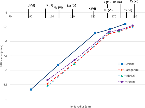
Figure 2. Lattice energies for possible polymorphs of alkali metal nitrates as indicated by filled symbols. Different crystal structures are shown in different colours: calcite (blue), aragonite (red), RbNO3 phase IV structure (green) ferroelectric trigonal (purple). The stable low temperature polymorphs are calcite (Li, Na), aragonite (K) and RbNO3 phase IV (Rb, Cs). The ionic radii come from Shannon [48]; Roman numerals denote the coordination number to which they refer. A comparison with previous force-fields [6–10] is given in the Supplementary Information.
Download figure:
Standard image High-resolution imageTable 6. Comparison between dielectric constants calculated using various force-fields and experimental values for the aragonite phase of potassium nitrate (KNO3).
| ε11 | ε22 | ε33 | |
|---|---|---|---|
| Expt [33] | 2.28 | 1.56 | 2.25 |
| Force-field (this work) | 3.6 | 2.9 | 2.8 |
| Force-field [6] | 1.79 | 2.55 | 2.47 |
| Force-field [7] | 0.5 | 2.17 | 2.11 |
| Force-field [8] | 3.5 | 4.24 | 3.95 |
| Force-field [9] | 2.58 | 2.22 | 2.33 |
| Force-field [10] | 2.6 | 2.86 | 2.66 |
*Note that the axes have been changed from the original references to conform to the crystallographic axes used for the Pnma space group in [18].
Table 7. Comparison between elastic stiffness constants (GPa), calculated using various force-fields and density functional calculations and experimental values for the aragonite phase of potassium nitrate (KNO3).
| C11 | C22 | C33 | C44 | C55 | C66 | C12 | C13 | C23 | |
|---|---|---|---|---|---|---|---|---|---|
| Expt [32] a,b | 26.1 | 49.7 | 40.7 | 10.5 | 9.6 | 7.0 | 12.8 | 14 | 22.1 |
| Force-field (this work) | 15.3 | 39.3 | 28.4 | 8.4 | 9.6 | 8.2 | 8.5 | 9.5 | 16.2 |
| Force-field [6] | 18.1 | 41.3 | 32.8 | 10.1 | 10.3 | 8.9 | 9.6 | 11 | 17.6 |
| Force-field [7] | 44.7 | 59.9 | 39.3 | 11.7 | 15.1 | 13.5 | 20.1 | 21.9 | 30.4 |
| Force-field [8] | 24.4 | 42.6 | 35.1 | 9.9 | 12.4 | 11.1 | 7.4 | 9 | 20 |
| Force-field [9] | 9.9 | 37.6 | 29.0 | 8.00 | 8.0 | 6.7 | 13.3 | 13.3 | 18.9 |
| Force-field [10] | 18.1 | 39.5 | 30.6 | 9.6 | 10.5 | 8.8 | 10.1 | 11.4 | 17.2 |
| DFT (this work) | 28.7 | 64.6 | 37.6 | 11.3 | 8.8 | 7.2 | 18.4 | 14.5 | 34.6 |
| DFT [44] | 21.9 | 40.2 | 32.9 | 9.6 | 8.8 | 7.3 | 10.4 | 12.1 | 17.3 |
a Note that the axes (and hence the Voigt notation) for the elastic constants has been changed from the original references to conform to the crystallographic axes used for the Pnma space group in [18]. b Values extrapolated back from the measured values at 293 K to 0 K using the thermo-elastic constants reported in the same paper [32].
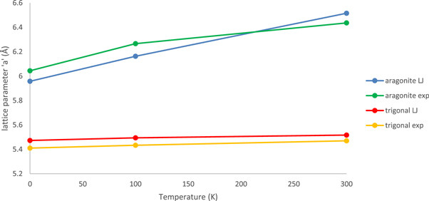
Figure 3. Lattice parameter fits for potassium nitrate (aragonite and trigonal (ferroelectric) structure).
Download figure:
Standard image High-resolution imageThe agreement with the experimental dielectric [33] and elastic constants (extrapolated to 0 K) [32] shown in tables 6 and 7 is as good as that obtained with previous sets of parameters where comparison is possible. Table 7 also shows that the forcefields compare reasonably well with the results of density functional calculations for the elastic properties. However, the new force-field improves on previous work in its ability to reproduce the experimental lattice dynamics. All previous force-fields show instabilities in the phonon spectra for at least some of the alkali nitrate polymorphs to which they were fitted except for those of Hammond [5]. This indicates that the structures obtained using previous force-fields were calculated using the full crystal symmetry and will distort away from the experimental crystal space group if the symmetry constraint is reduced or removed.
To obtain the interaction between the nitrate anion and the water molecules, we fit to the experimental crystal structure of the only known hydrate of the alkali metal nitrates, LiNO3.3H2O [45]. We assume the lithium interactions given in tables 1 and 5, the nitrate model of table 2 and the water model of table 4. We use mixing rules for the interactions between the nitrate oxygen and water oxygen atoms. This leaves only the interaction between the hydrogen atoms of water and the oxygen atoms of the nitrate ion to fit. All the parameters for the interactions between water and the nitrate ion are given in table 8 and the comparison with the structure of LiNO3.3H2O in table 9 with further details given in the Supplementary Information.
Table 8. Interactions between water and the nitrate anion using a Buckingham potential form 
| Interactions | A(eV) |
 (Å) (Å) | C(eV Å6) |
|---|---|---|---|
| H(H2O)-O(NO3 −) | 577.7 | 0.226352 | 0.0 |
| O(H2O)-O(NO3 −) | 225677 | 0.18661 | 29.0 |
Table 9. Comparison with structural data for LiNO3.3H2O (space group Cmcm (63)) [45]. Comparison of the atomic positions can be found in Supplementary Information.
| Lattice parameters | Expt | Force-field |
|---|---|---|
| a (Å) | 6.8018 | 6.7756 |
| b (Å) | 12.7132 | 12.7464 |
| c (Å) | 5.9990 | 5.9296 |
2.3. Simulation of free energies of hydration and solution structure
To demonstrate the reliability of the force field, we have calculated the free energy of hydration of the potassium and nitrate ions using the thermodynamic integration method described in the Methodology section. We must first consider the data which we are to use for the comparison. It is not possible to use experiments to measure the free energy of hydration of isolated ions; what can be measured is the thermodynamics of neutral combinations of ions. This can be used to infer the hydration free energies of isolated ions provided that the hydration free energy of one species can be fixed. The species chosen is usually the proton. So-called 'conventional' free energies are obtained by setting this quantity to zero. However, the free energies obtained by this route cannot be directly compared with simulations because of the arbitrary nature of this assumption. Hence a physically-based model must be used, usually based on the Born model of hydration. These issues are discussed in depth from the experimental perspective by Marcus [46, 47, 49], who is the author of the most extensive tables of thermodynamic parameters for the hydration of ions and more recently by Hofer and Hünenberger [50] from a theoretical perspective. Marcus [47] fixed the absolute free energy of a hydration for a proton at 298.15 K as −1056 ± 6 kJ mol−1. It is now generally agreed from both theoretical [50] and experimental [51] research that a more accurate value is −1100 ± 14 kJ mol−1. Marcus' tabulated values must therefore be corrected by −44z kJ mol−1 where z is the charge of the ion. So his free energy of hydration for potassium (−295 kJ mol−1) should be corrected to −339 kJ mol−1 and his free energy of hydration for the nitrate ion (−300 kJ mol−1) should be corrected to −256 kJ mol−1.
Corrections must also be made to the simulation result. This is true whether spherical or periodic boundary conditions are used [52]. For periodic boundary conditions, the simulation of free energies of ion hydration uses a charged simulation cell, producing a divergence in the electrostatic summation which must be removed. The simplest way of doing this is to add a uniform neutralising correction to cancel the charge. This involves two types of correction. The first, (due to Fuchs [53]), corrects for the interaction of the charges with the neutralising background. The second (first discussed in [54], but usually called the Wigner correction) corrects for the self-energy of the added charge with its periodic images. Most codes using P3M (particle-particle-particle-mesh) approaches (such as LAMMPS, AMBER, DL_POLY) already include these terms, although this may not be immediately apparent (see [55] especially appendix A). Such codes do not include corrections for the artificial polarisation effects caused by the periodic boundary conditions. These are discussed in [56, 57]. Moreover, to connect with the absolute values for individual ions obtained by Marcus and others, we must ignore any effects due to the transfer of the ion through the interface between the gas and water phases and subtract any effects due to the errors in the electrostatic potential at the site of the ion generated by the summation convention used for the electrostatics (see [51, 57, 58] for a full discussion and the importance of the distinction between 'real' and 'intrinsic' quantities when comparing with Marcus' tables). There are also some small corrections arising from choice of thermodynamic conventions [47, 57]. Details are given in the Supplementary Information.
The raw thermodynamic integration results give −297 kJ mol−1 for the free energy of hydration of the potassium ion (the same as the value obtained by Joung and Cheatham [26] using the SPC/E model for water♯). A hydration free energy of −311 kJ mol−1 was obtained for the nitrate ion. When the corrections are applied, these values become −372.5 kJ mol−1 (corrected Marcus value −339 kJ mol−1) for the potassium ion and −217.5 kJ mol−1 (corrected Marcus value −256 kJ mol−1) for the nitrate ion. However, it is important to remember that experimentally accessible quantities (such as the free energy of solution) depend only on the sum of the free energies of hydration of individual ions. Both the simulation corrections (arising from the electrostatic potential for the cation and anion) and the experimental corrections (arising from the choice of the free energy of hydration of the proton) cancel out. The simulated value for the sum of the free energies of cation and anion is −585 kJ mol−1. The tabulated value obtained from Marcus is −595kJ mol−1 - within about 2% showing excellent agreement.
Further tests using the force-field in water have been performed. Starting from a box of water and potassium nitrate, molecular dynamics simulations using DL_POLY in an NVT ensemble have been performed (2000 water molecules and 50 potassium nitrate formula units). The radial distribution function (RDF) for KNO3-water was extracted and analysed (see figure 3). The first maximum in the RDF for the nitrogen in the nitrate ion and the oxygen in the water molecule (rmax (N–Ow)) is at 3.59 Å, which shows good agreement with those found in literature, as can be seen from table 10.
Table 10. Comparison between rmax(N-Ow) obtained in this work and available data in literature.
| rmax (N–Ow) | |
|---|---|
| Experimental [59] | 3.5 ± 0.311 Å |
| Xie et al [7] | 3.65 Å |
| Dang et al [60] | 3.40 Å |
| Banerjee et al [61] | 3.50 Å |
| This work | 3.59 A |
The number of water oxygen atoms around the nitrate nitrogen has also been calculated, by integrating the RDF. The coordination number obtained (9.6) shows a good agreement with the values from previous literature as it is possible to see in table 11.
Table 11. Comparison between coordination number obtained in this work and available data in literature.
| Coordination number | |
|---|---|
| Xie et al [7] | 10 ± 1 |
| Dang et al [60] | 12 |
| Banerjee et al [61] | 9.2 |
| This work | 9.6 |
♯The most important correction omitted by Joung and Cheatham is the one involving the electrostatic potential at the site of the cation. When this is added, their result for the free energy of hydration of the potassium ion becomes −371 kJ mol−1.
2.4. Simulation of the crystal structures at high temperature
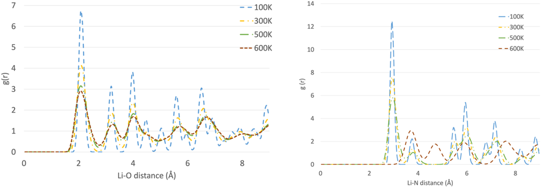
We finally turn to a more detailed consideration of the structures predicted by the simulations. NPT molecular dynamics simulations were performed as previously described and showed that for the lithium nitrate system the structure is calcite-like (space group R  c) at all temperatures and peaks retain their shape (figure 4). The structure loses some long-range order when the system is heated up from 100 K to 500 K (peaks between 4.5 and 5 Å and between 5 and 7.8 Å merge). However, changes in the polymorph are not visible (lithium nitrate is monotropic as experimentally reported). If the temperature is raised to 600 K the long-range order decays further (peaks shift to the right/broaden and their height decreases). At greater atomic separations, the lack of coherence becomes more evident with more peaks merging (around 6, 7 and 9 Å). The behaviour is similar for sodium nitrate (figure 5). At all temperatures the structure is calcite-like (space group R
  c); the peaks lose their shape as the temperature rises.
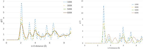
Figure 4. Radial distribution functions for Li-O (left) and Li-N (right) in LiNO3.
Download figure:
Standard image High-resolution image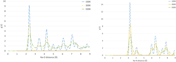
Figure 5. Radial Distribution Function for Na - O (left) and Na - N (right) in NaNO3.
Download figure:
Standard image High-resolution imagePotassium nitrate is a more interesting case to study, because the RDFs show evidence for three different polymorphs (see figure 6): the ferro-electric trigonal structure (space group R3m) at 100 K; the aragonite structure at 300 K and the trigonal R  m structure, (quasi-calcite form) at 500 K. On cooling down the system returns to the original structure but not directly. Cooling down the 500 K trigonal structure gives a distorted aragonite structure, whereas the 300 K structure returns to the ferro-electric trigonal form on further cooling. This suggests that the force field is able to reproduce the polymorph changes and shows that those changes are temperature-dependent (potassium nitrate is enantiotropic). Figure 7 shows the good agreement between the experimental K-O distances obtained by X-ray diffraction and those obtained by simulation.

Figure 6. Radial Distribution Function for K - N in KNO3 as the temperature increases. The red line represents the system at 100 K, the orange line at 300 K, the purple line at 500 K and the green line at 650 K.
Download figure:
Standard image High-resolution image
Figure 7. Radial Distribution Function for K-O in KNO3 obtained by cooling down the simulation at 500 K (blue) and the RDF of the polymorph obtained from cooling down the aragonite structure (red). Dotted lines represent the positions of XRD peaks for the experimental R3m structure [13].
Download figure:
Standard image High-resolution image
3. Conclusions
In this paper we discussed the need for a reliable, transferable force field for the alkali metal nitrates that can be used for all the nitrates including solid solutions. Our force-field reproduces the order of stability of the polymorphs for each alkali nitrate, the crystal structures of the polymorphs together with the elastic and dielectric properties of the materials where these are available. Stable phonon spectra (i.e. no imaginary modes) are obtained in all cases. The model also behaves well as a function of temperature, reproducing the experimental lattice expansion and also showing the transformation of the structures to disordered forms (due to the thermally activated rotation of the nitrate groups) where appropriate. The model is also compatible with the well-known model of Joung and Cheatham [26] for alkali metal ions in solution. Future work will demonstrate the application of this model to aqueous interfaces and crystallisation.
Acknowledgments
We acknowledge the Engineering and Physical Sciences Research Council (EPSRC) for funding via Programme Grant No. EP/R018820/1 which funds the 'Crystallisation in the Real World' Consortium. Via our membership of the UK's HEC Materials Chemistry Consortium, which is funded by EPSRC (EP/R029431), this work used the ARCHER2 UK National Supercomputing Service (http://www.archer2.ac.uk). VF thanks EPSRC for the provision of a studentship. For the purpose of open access, the author has applied a Creative Commons Attribution (CC BY) licence to any Author Accepted Manuscript version arising
Data availability statement
All data that support the findings of this study are included within the article (and any supplementary files).
Associated content
Supplementary information: Calculating the corrections to the free energy of hydration, comparison of force-fields with crystal structures, stability of polymorphs, comparison with crystal properties, the lattice thermal expansion and RDF functions (PDF)
Conflict of interest statement
The authors declare that there are no conflicts of interest.