Isotope detection in molecules with ultrafast electron diffraction and rotational spectrometry

Gas electron diffraction (GED), where a continuous electron beam is scattered from a sample of molecules in a gas beam, is a well-established method to determine the structure of isolated molecules [1, 2]. Gas phase ultrafast electron diffraction (GUED) has become a powerful tool to determine changes in molecular structures on femtosecond and picosecond time scales [3–5]. In GUED, a pump laser pulse triggers a reaction, and a probe electron pulse is used to capture the structure as a function of time delay after the excitation. Recent advances have pushed the temporal resolution to the femtosecond scale where coherent nuclear motions can be spatially and temporally resolved [6–8]. GUED has also been used to probe the dynamics of rotational wavepackets, where the pump laser pulse impulsively aligns the molecules, and the angular distribution is probed by the electron pulses. The diffraction signal from aligned molecules had been theoretically predicted [9] and demonstrated experimentally for the case of adiabatic alignment using nanosecond electron pulses [10], for selective alignment using picosecond electron pulses [11] and for impulsive alignment using femtosecond electron pulses [12]. The anisotropy in the diffraction pattern can be used to retrieve information about the angular distribution. In addition, GUED from aligned molecules allows for the retrieval of three-dimensional molecular structures [12, 13] and to capture the dynamics of rotational wavepackets on femtosecond time scales [14, 15, 16].

The structural information contained in a GED pattern is the interatomic distance between all atom pairs in the molecule. However, not all distances can be resolved due to the finite spatial resolution of the measurement. In GED, this information is combined with quantum chemical calculations and infrared spectroscopy to determine the molecular structure. In GUED, the ground state structure of the molecule is known, and the structural changes can be inferred from the changes in the diffraction patterns, often with the support of theory [6–8, 17]. The electron diffraction signal originates from the charge distribution in the molecule [18], and therefore it is not sensitive to the number of neutrons and cannot distinguish between different isotopologues (molecules where one or more atoms are substituted by an isotope). Here we show that by analyzing the time-dependence of GUED patterns from non-adiabatically laser-aligned molecules, it is possible to distinguish between isotopologues. Other methods such as mass spectrometry, can distinguish between isomers but are not sensitive to structure. This is a key advantage of this GUED measurement, which provides both the structure and the isotopic composition in a single measurement. By following the rotational dynamics, we can determine the abundance of ³⁵Cl and ³⁷Cl in a sample of CH₃Cl molecules.

Nonadiabatic alignment of molecules by ultrashort laser pulses has been studied in recent years theoretically [19–23] and experimentally by the use of ion imaging [24–28] and used to determine the angular dependence of ionization [29]. Molecules interact with the laser through an induced dipole, and receive an impulsive 'kick' from the laser. The laser generates a rotational wave packet resulting in prompt alignment, followed by dephasing and periodic revivals of the alignment. In the nonadiabatic alignment regime, the pulse duration of the laser field is much shorter than the rotational timescale of the molecule, and the peak alignment of the ensemble is obtained shortly after the interaction of the molecules with the laser pulse [15]. In the case of linear and symmetric top molecules, the phase of the rotational wave packet creates rotational revivals where the angular distribution changes between alignment and anti-alignment [15, 30, 31]. The rotational period is determined by the moment of inertia, which is sensitive to both the molecular structure and the mass of the constituent atoms. Thus, a measurement of the rotational period is in principle sensitive to isotope substitution. The application of this technique is not limited to the case of linear and symmetric top molecules. In principle, molecules with small differences in the moment of inertia can be distinguished using this technique, time-resolved rotational spectrometry (TRRS). We demonstrate GUED-based TRRS experimentally by applying the method to a mixture of CH₃ ³⁵Cl and CH₃ ³⁷Cl molecules. Based on the rotational revivals, the method distinguishes between the two isotopologues and provides an accurate measurement of the rotational periods and relative abundances.

2.1. Nonadiabatic alignment of a symmetric top

The theory of nonadiabatic molecular alignment by ultrashort intense laser pulses has been described previously [19–23]. Here we give a brief overview of the alignment of prolate symmetric top molecules induced by a linearly polarized laser field. The laser induced impulsive alignment can be described by the time-dependent Schrödinger equation using an effective Hamiltonian containing a rotational Hamiltonian and a Hamiltonian due to the induced dipole interaction: $H\left(t\right)={H}_{{\rm{rot}}}+{H}_{{\rm{ind}}}.$

$$\begin{eqnarray}&&i\hslash \displaystyle \frac{\partial {\rm{\Psi }}(t)}{\partial t}=H(t){\rm{\Psi }}(t)\end{eqnarray} \tag{ 1 }$$

$$\begin{eqnarray}&&{H}_{{\rm{ind}}}=-\displaystyle \frac{1}{4}{ {\mathcal E} }^{2}\left(t\right){\rm{\Delta }}\alpha \,{\cos }^{2}\theta ,\,{\rm{\Delta }}\alpha ={\alpha }_{\parallel }-{\alpha }_{\perp }\end{eqnarray} \tag{ 2 }$$

where ${\alpha }_{\parallel }$ and ${\alpha }_{\perp }$ are the polarizability tensor components along the directions parallel and perpendicular to the molecular axis; ${\mathcal E} (t)$ is the envelope of the electric field of the laser pulse, $\theta$ is the angle between molecular axis and the laser polarization, and ${\rm{\Psi }}(t)$ is the rotational wavefunction. In the case of a prolate symmetric top the rotational hamiltonian takes the form ${H}_{{\rm{rot}}}={C}_{{\rm{e}}}{{\boldsymbol{J}}}^{2}+({A}_{{\rm{e}}}-{C}_{{\rm{e}}}){J}_{z}^{2},$ where ${A}_{{\rm{e}}}\gt {C}_{{\rm{e}}}$ and the rotational constants are given by ${A}_{{\rm{e}}}={\hslash }^{2}/2{I}_{{\rm{aa}}}\,$and ${C}_{{\rm{e}}}={\hslash }^{2}/2{I}_{{\rm{cc}}}.$ Here ${I}_{{\rm{aa}}}$ and ${I}_{{\rm{cc}}}$ are the principal moments of inertia of the molecule. The wavefunction ${\rm{\Psi }}(t)$ can be expanded as ${{\rm{\Psi }}}_{{J}_{i}{K}_{i}{M}_{i}}\left(t\right)=\displaystyle {\sum }_{JK}{C}^{JK{M}_{i}}(t)\left|JK\right.\left.{M}_{i}\right\rangle$ using the symetric top eigenfunctions as a basis set, where $\left|{J}_{i}{K}_{i}\right.{M}_{i}\gt$ are intial states with the Boltzmann distribution ${W}_{{J}_{i}{K}_{i}{M}_{i}}\left(T\right)$ determined by the temperature of the ensemble. Ref. [19]. shows that

$$\begin{eqnarray}&&\begin{array}{l}i\hslash {\dot{C}}^{JK{M}_{i}}\left(t\right)=\displaystyle \sum _{J^{\prime} ,\,K^{\prime} }{C}^{{J}^{^{\prime} }{K}^{^{\prime} }{M}_{i}}\left(t\right)\cdot {\delta }_{KK^{\prime} }\left\{{E}^{{J}^{^{\prime} }{K}^{^{\prime} }}{\delta }_{J{J}^{^{\prime} }}-\frac{2}{3}\frac{{ {\mathcal E} }^{2}\left(t\right){\rm{\Delta }}\alpha }{4}JK{M}_{i}| {D}_{00}^{2}| {J}^{^{\prime} }{K}^{^{\prime} }{M}_{i}\right\}\\ \,=\,\displaystyle \sum _{{J}^{{\prime} }}{C}^{{J}^{^{\prime} }K{M}_{i}}\left(t\right)\cdot \left\{{E}^{JK}{\delta }_{J{J}^{^{\prime} }}-\frac{2}{3}\frac{{ {\mathcal E} }^{2}\left(t\right){\rm{\Delta }}\alpha }{4}JK{M}_{i}| {D}_{00}^{2}| J^{\prime} K{M}_{i}\right\}\end{array}\end{eqnarray} \tag{ 3 }$$

where ${D}_{00}^{2}$ is the rotational matrix defined in [32]. The differential equation indicates that the selection rule is $\left|J-2\right|\leqslant J^{\prime} \leqslant J+2,$ and both the quantum number K and M do not change during the interaction of the molecule with the laser field. The coefficients ${C}^{JK{M}_{i}}\left(t\right)$ can be calcualted numerically by using the basis function $\left|JK\right.\left.M\right\rangle ={\left(\tfrac{2J+1}{8{\pi }^{2}}\right)}^{\tfrac{1}{2}}{e}^{iM\phi }{d}_{MK}^{J}(\theta ){e}^{iK\chi },$ where $\phi ,\theta ,\chi$ are the Eular angles and ${d}_{MK}^{J}(\theta )$ is the Wigner's d-matrix [32].

After the interaction, the wavepacket evolves in free space with ${{\rm{\Psi }}}_{{J}_{i}{K}_{i}{M}_{i}}\left(t\right)=\displaystyle {\sum }_{J}{c}^{J{K}_{i}{M}_{i}}{e}^{-i\displaystyle \frac{{E}^{J{K}_{i}}}{\hslash }t}\left|J{K}_{i}\right.\left.{M}_{i}\right\rangle ,$ where ${c}^{J{K}_{i}{M}_{i}}$ are the coefficients when the laser field is turned off, correcponding to the ${C}^{JK{M}_{i}}\left(t\right)$ at the end, and ${E}^{J{K}_{i}}={C}_{{\rm{e}}}J(J+1)+({A}_{{\rm{e}}}-{C}_{{\rm{e}}}){K}_{i}^{2}.$ The corresponding probability density is

$$\begin{eqnarray}&&{\left|{\Psi }_{{J}_{i}{K}_{i}{M}_{i}}\left(t\right)\right|}^{2}=\displaystyle \sum _{J^{\prime} J^{\prime\prime} }{c}^{{J}^{^{\prime} }{K}_{i}{{M}_{i}}^{* }}{c}^{J^{\prime\prime} {K}_{i}{M}_{i}}{e}^{-i\frac{{\rm{\Delta }}{E}_{{J}^{^{\prime} }{J}^{^{\prime\prime} }}}{\hslash }t}\left|{J}^{^{\prime} }{K}_{i}\right.{{M}_{i}}^{* }{J}^{^{\prime\prime} }{K}_{i}{M}_{i}\end{eqnarray} \tag{ 4 }$$

where ${\rm{\Delta }}{E}_{{J}^{^{\prime} }{J}^{^{\prime\prime} }}={C}_{{\rm{e}}}\left[J^{\prime} \left(J^{\prime} +1\right)-J^{\prime\prime} \left(J^{\prime\prime} +1\right)\right]=2n{C}_{{\rm{e}}}.$ This implies that there will be revivals of the alignment with period $\tau =\tfrac{\pi \hslash }{{C}_{{\rm{e}}}}=\tfrac{2\pi {I}_{{\rm{cc}}}}{\hslash },$ which has the same form as the revival period for linear molecules shown in [33]. The degree of alignment of the molecular ensemble is defined as

$$\begin{eqnarray}&&{\cos }^{2}\theta t=\displaystyle \sum _{{J}_{i},{K}_{i},{M}_{i}}{W}_{{J}_{i}{K}_{i}{M}_{i}}\left(T\right){\Psi }_{{J}_{i}{K}_{i}{M}_{i}}\left(t\right)| \,{\cos }^{2}\theta | {\Psi }_{{J}_{i}{K}_{i}{M}_{i}}\left(t\right)\end{eqnarray} \tag{ 5 }$$

where i indicates all the possible initial states. The probability density of the ensemble for one-dimensional alignment has no dependence on $\phi ,\chi$ due to the conservation of J and M during the interaction.

$$\begin{eqnarray}&&\rho \left(\theta ,t\right)=\displaystyle \sum _{{J}_{i},{K}_{i},{M}_{i}}{W}_{{J}_{i}{K}_{i}{M}_{i}}\left(T\right)\displaystyle {\int }_{0}^{2\pi }\displaystyle {\int }_{0}^{2\pi }{\left|{{\rm{\Psi }}}_{{J}_{i}{K}_{i}{M}_{i}}\left(t\right)\right|}^{2}d\phi d\chi \end{eqnarray} \tag{ 6 }$$

Due to the periodicity of (4), both $\left\langle {\cos }^{2}\theta \right\rangle \left(t\right)$ and $\rho \left(\theta ,t\right)$ are periodic functions with period τ. The period of the revivals will depend not only on the structure but also on the mass of the constituent atoms. Small changes in the rotational period due to isotopic substitutions can be most easily detected by following the signal for multiple rotational periods where the absolute time difference in the revivals will be larger. TRRS could be used to distinguish asymmetric top molecules with isotopic substitutions as well though the theory is more complicated and numerical simulation is required.

2.2. Electron diffraction

The intensity of electrons scattered from a molecular ensemble is an incoherent sum of the scattering from individual molecules, in which electron waves scattered from atoms interfere. For the case of rigid molecules aligned along one single axis (one dimensional alignment) with angular distribution $g\left(\vartheta \right),$ the total intensity on the detector can be written as [14]

$$\begin{eqnarray}&&{I}_{{\rm{total}}}={\iint }^{\,}\displaystyle \sum _{j=1}^{n}\displaystyle \sum _{k=1}^{n}{f}_{j}^{* }(s){f}_{k}\left(s\right){e}^{-i\vec{s}\cdot {\vec{r}}_{jk}\left(\vartheta ,\varphi \right)}\,{g}_{jk}\left(\vartheta \right)\sin \,\vartheta \,{\rm{d}}\vartheta \,{\rm{d}}\varphi \end{eqnarray} \tag{ 7 }$$

where n is the total number of atoms in the molecule, ${f}_{k}\left(s\right)$ is the form factor of the kth atom, $\vec{s}$ is the momentum transfer vector, ${\vec{r}}_{jk}$ is the distance vector from the jth atom to the kth atom, $(\vartheta ,\varphi )$ are the polar and azimuthal angles, respectively, that indicate the orientation of the vector ${\vec{r}}_{jk}.$ ${g}_{jk}\left(\vartheta \right)$ is the angular distribution of the vector ${\vec{r}}_{jk}.$ The $j=k$ terms in the summation correspond to the atomic scattering intensity I_at, while the $j\ne k$ terms constitute the molecular scattering intensity I_mol that contains the interference of all atomic pairs in the molecule. For a random angular distribution, the integral of equation (7) can be simplified to [34]

$$\begin{eqnarray}&&{I}_{{\rm{total}}}^{{\rm{random}}}=\displaystyle \sum _{j=1}^{n}\displaystyle \sum _{k=1}^{n}{f}_{j}^{* }(s){f}_{k}\left(s\right)\displaystyle \frac{\sin (s{r}_{jk})}{s{r}_{jk}}\end{eqnarray} \tag{ 8 }$$

where s is the amplitude of the momentum transfer vector, ${r}_{jk}$ is the distance between the jth and kth atom. We calculate a difference-diffraction signal ${\rm{\Delta }}{I}_{{\rm{mol}}}\left({s}_{x},{s}_{y},t\right)$ by subtracting a diffraction pattern of randomly oriented molecules from the time dependent diffraction pattern of aligned molecules. This removes the contribution from the atomic scattering intensity and highlights the anisotropic part of the diffraction signal

$$\begin{eqnarray}&&{\rm{\Delta }}{I}_{{\rm{mol}}}\left({s}_{x},{s}_{y},t\right)={I}_{{\rm{total}}}\left({s}_{x},{s}_{y},t\right)-{I}_{{\rm{total}}}^{{\rm{random}}}\left({s}_{x},{s}_{y}\right)={I}_{{\rm{mol}}}\left({s}_{x},{s}_{y},t\right)-{I}_{{\rm{mol}}}^{{\rm{random}}}\left({s}_{x},{s}_{y}\right)\end{eqnarray} \tag{ 9 }$$

A femtosecond laser pulse is used to create a rotational wavepacket in a sample of CH₃Cl molecules, and a synchronized femtosecond electron pulse is used to probe the angular distribution as a function of time. We use a 90 kiloelectronvolt ultrafast electron diffraction (keV UED) setup to measure the rotational revivals of chloromethane isotopologues CH₃ ³⁵Cl and CH₃ ³⁷Cl induced by an infrared ultrafast laser pulse. The chloromethane sample was purchased from Sigma-Aldrich with chemical purity ≥ 99.5% and introduced into the vacuum in a molecular jet. The details of the keV UED setup have been described in previous publications [14, 35]. The laser systems outputs femtosecond pulses with maximum energy of 2 mJ at a repetition rate of 5 kHz. Each laser pulse is split into a pump beam to align the molecules and a probe beam to generate the electron pulses. The pump laser pulse has a pulse duration of 200 fs, a spot size of 190 μm (horizontal) × 260 μm (vertical), and pulse energy of 0.8 mJ. The intensity front of the laser pulse is tilted to minimize the group velocity mismatch between laser and electron pulses and improve the instrument response time [36]. The probe laser pulse, with an energy of 0.17 mJ, is frequency tripled to a wavelength of 266 nm to trigger electron emission from a copper photocathode. The photoelectron pulse is first accelerated to 90 keV using a static electric field, and then longitudinally compressed using 3 GHz radio-frequency field to minimize the duration at the sample. A platinum aperture with a diameter of 200 μm is used to collimate the electron beam. The average electron beam current on the sample is 20 picoamperes, which corresponds to 25,000 electrons per pulse. The instrumental temporal resolution was previously determined to be 240 fs using a pump laser with a pulse duration of 60 fs in [14]. In this experiment, the laser pulse duration was increased to 200 fs to reduce the intensity and avoid ionization, thus we expect a slightly broader temporal resolution of around 300 fs. The chloromethane sample is mixed with a carrier gas, helium, at a ratio of 1:1. We use a de Laval nozzle with an inner diameter of 30 μm and backing pressure of 1050 mbar to deliver the sample to the interaction region as a supersonic gas jet. The scattering patterns are recorded using a phosphor screen that is imaged on an electron-multiplying charge-coupled device (EMCCD). The exposure time of each image during a scan is 8 s, and multiple images are recorded at each delay point.

Figures 1(a)–(e) shows the 2D diffraction-difference patterns ${\rm{\Delta }}{I}_{{\rm{mol}}}\left({s}_{x},{s}_{y},t\right)$ at five different time points: (a) the prompt alignment peak (where time zero t = 0 is defined), (b) t = 0.4 ps (still within the prompt alignment but the anisotropy is already decreasing), (c) t = 0.8 ps (after the prompt alignment peak when the anisotropy approaches zero), (d) t = 18.4 ps (the peak of the first half-revival), and (e) t = 19.18 ps (the trough of the first half-revival), respectively. Forty images with an integration time of 8 s for each image were acquired and averaged for each time delay. The changes in the angular distribution are reflected in the azimuthal angular dependence of the intensity distribution in the diffraction signal. The prompt alignment peak corresponds to the molecular axis (the C-Cl axis) lining up along the direction of the laser polarization. The patterns in figures 1(a), (b), (d) correspond to a distribution aligned along the direction of the laser polarization, while figure 1(e) shows the pattern corresponding to anti-alignment, i.e. molecules aligned perpendicular to the direction of the laser polarization and figure 1(c) corresponds to the quasi random angular distribution due to dephasing of the wavepacket between revivals. Note that dephasing does not produce a truly random orientation, a small anisotropy is always present.

Zoom In Zoom Out Reset image size

Here we show how to simulate the diffraction patterns of aligned molecules. The probability density of the molecule ensemble at time t is ${\left(\tfrac{1}{2\pi }\right)}^{2}\rho (\theta ,t),$ which is calculated using the simulated wave packets from the nonadiabatic alignment with theory in section 2.1. The initial J_max estimated for the ensemble is 30. We calculated 31 populated excited states for each initial state after interaction with the laser, and there are 9 excited states with coefficients that are not negligible. The diffraction pattern from aligned molecules is calculated by weighting the diffraction intensities of a single molecule at different orientations with the corresponding probability density, formulated as

$$\begin{eqnarray}&&{I}_{{\rm{mol}}}=\displaystyle {\int }_{0}^{2\pi }\displaystyle {\int }_{0}^{2\pi }\displaystyle {\int }_{0}^{\pi }{I}_{{\rm{mol}}}^{{\rm{S}}}\left(\phi ,\theta ,\chi \right)\,{\left(\displaystyle \frac{1}{2\pi }\right)}^{2}\rho (\theta ,t)\,\sin \,\theta \,d\theta d\phi d\chi \end{eqnarray} \tag{ 10 }$$

where ${I}_{{\rm{mol}}}^{{\rm{S}}}(\phi ,\theta ,\chi )$ is the diffraction pattern of the molecule at the orientation described by the Euler angles. The total diffraction pattern is ${I}_{{\rm{total}}}={I}_{{\rm{mol}}}+{I}_{{\rm{at}}}.$ The ${\cos }^{2}\theta \left(t\right)$ is calculated using equation (5). Figure 2 shows the simulated and experimental temporal evolution of the anisotropy in the diffraction signal. The laser parameters in the experiment are used to simulate the temporal evolution of anisotropy for CH₃ ³⁵Cl and CH₃ ³⁷Cl molecules with the structure of the molecule optimized using ORCA [37] and the level of theory (B3LYP, DEF2-SVP). The rotational temperature of the molecular ensemble is estimated to be 50 K based on previous operation of our gas jet. The anisotropy of each diffraction pattern shown in figure 1 is calculated using the experimental ${I}_{{\rm{total}}}\left({s}_{x},{s}_{y},t\right)$ as Ani = (S_H − S_V)/(S_H + S_V), where S_H and S_V are the total detector counts in the range 1.4 Å⁻¹ < s < 3 Å⁻¹ within horizontal and vertical cones with an opening angle of 60 degrees.

Zoom In Zoom Out Reset image size

Figure 2(a) shows the simulated anisotropy for the two molecules CH₃ ³⁵Cl and CH₃ ³⁷Cl calculated separately and displayed together in the same graph. The maximum degree of alignment at the revival peak is 0.45. For the prompt peak and the first revivals, the alignment peaks overlap very closely, i.e. the time difference between the revivals is smaller than the duration of each revival. As the revival index increases (first, second, third revival, etc) the difference in the rotational periods can be seen more clearly. In order to compare with the data, the anisotropy is scaled by an excitation factor of 0.45, which accounts for the spatial overlap of the laser and electron pulses on the sample. The excitation factor is obtained by comparing the amplitudes of simulated and experimental anisotropy. The relative abundances of ³⁵Cl and ³⁷Cl are 75.76% and 24.24%, respectively [38–40]. The reported values are used to calculate the total anisotropy using the equation ${{\rm{Ani}}}_{{\rm{total}}}({\rm{t}})=75.76 \% \,\times {{\rm{Ani}}}_{{{{\rm{CH}}}_{3}}^{35}{\rm{Cl}}}({\rm{t}})+24.24 \% \times {{\rm{Ani}}}_{{{{\rm{CH}}}_{3}}^{37}{\rm{Cl}}}({\rm{t}}),$ for each time step. Figure 2(b) shows the temporal evolution of ${\,\mathrm{Ani}}_{{\rm{total}}}({\rm{t}}).$ For the first few revivals, the signal has a complex structure as the revivals from the isotopologues are overlapped, however, for times longer than 200 ps, the revivals start to separate in time and resemble a double revival structure. Note that due to the different relative abundance of the two isotopes, the two revivals have different amplitudes.

Figure 2(c) shows the experimental anisotropy Ani_exp(t), with the revival indices listed on the top part of the figure. The experimental signal very closely matches the simulated anisotropy signal in figure 2(b). For the data acquisition, each time step corresponds to a single image with acquisition time of 8 s. A variable time step was used with a time step of 133.33 fs near the revivals and 3.33 ps for the region between the revivals.

We now show that rotational periods, mass difference, and relative abundance of the two isotopologues can be retrieved from the experimental data. We use the difference in the timing of the revivals in the experimental anisotropy to calculate the rotational period of CH₃ ³⁵Cl and CH₃ ³⁷Cl. The rotational period can be written as $\tau =\tfrac{2\pi {I}_{{\rm{cc}}}}{\hslash }=\tfrac{{\rm{\Delta }}t}{{\rm{\Delta }}N},$ where ${\rm{\Delta }}t$ is the time delay difference between two revival peaks in the experimental data and ${\rm{\Delta }}N$ is the difference of revival indices.

We assume that the two isotopologues have the same structure and use the principal axes of inertia to calculate ${I}_{{\rm{cc}}}.$ Let the x axis be along the axis of the molecule (C-Cl), with the y and z axes perpendicular to it, and the origin at the center of mass of the molecule. The moment of inertia is ${I}_{cc}=\displaystyle {\sum }_{k}{m}_{k}({x}_{k}^{2}+{y}_{k}^{2}),$ where k indicates all the constituent atoms. Since the changes are small $\tfrac{\delta {m}_{{\rm{Cl}}}}{{m}_{{\rm{Cl}}}}\cong 0.057\ll 1$ and $\left|\tfrac{\delta {x}_{k}}{{x}_{k}}\right|\leqslant \left|\tfrac{\delta {x}_{{\rm{Cl}}}}{{x}_{{\rm{Cl}}}}\right|\cong 0.046\ll 1,$ we calculate the variation of ${I}_{{\rm{cc}}}$ by keeping the first order terms $\delta {I}_{cc}=\delta {m}_{{\rm{Cl}}}\cdot {x}_{Cl}^{2}+2\displaystyle {\sum }_{k}{m}_{k}\cdot {x}_{k}\cdot \delta {x}_{k}.$ Here $\delta {m}_{k}=0$ for $k\ne {\rm{Cl}},$ ${y}_{{\rm{Cl}}}^{2}=0,$ $\delta {y}_{k}^{2}=0$ are used to obtain the equation. Also, the shift of the ${x}_{k}$ due to the change of center of mass position shows that $\delta {x}_{k}=-\delta {x}_{{\rm{MC}}},$ where $\delta {x}_{{\rm{MC}}}$ is the shift of center of mass. Since the origin of the coordinate is at the center of mass, we have $\displaystyle {\sum }_{k}{m}_{k}\cdot {x}_{k}=0$ and $\delta {I}_{{\rm{cc}}}=\delta {m}_{{\rm{Cl}}}\cdot {x}_{{\rm{Cl}}}^{2}.$ Therefore, the mass difference between the isotopes $\delta {m}_{{\rm{Cl}}}$ can be obtained from the difference in the rotational periods $\delta \tau :$

$$\begin{eqnarray}&&\delta \tau =\displaystyle \frac{2\pi }{\hslash }\cdot \delta {I}_{{\rm{cc}}}=\displaystyle \frac{2\pi }{\hslash }\cdot {x}_{{\rm{Cl}}}^{2}\cdot \delta {m}_{{\rm{Cl}}}\end{eqnarray} \tag{ 11 }$$

where $\left|{x}_{{\rm{Cl}}}\right|$ is the distance from the Cl atom to the center of mass of the molecule. The error due to the approximation is estimated to be about 4% by using the known structure of chloromethane, which is way smaller than the uncertainty (19%) of the measured $\delta {m}_{{\rm{Cl}}}$ in table 1.

Table 1. Measurement of rotational period of CH₃ ³⁵Cl to CH₃ ³⁷Cl, mass difference, and abundance ratio. The theoretically calculated rotational periods, mass difference, and abundance ratio from [38–40] are listed for comparison.

	${\tau }_{{{{\rm{CH}}}_{3}}^{35}{\rm{Cl}}}$ (ps)	${\tau }_{{{{\rm{CH}}}_{3}}^{37}{\rm{Cl}}}$ (ps)	$\delta {m}_{{\rm{Cl}}}$ (amu)	Abundance ratio
Measurement	38.08 ± 0.11	38.79 ± 0.08	2.28 ± 0.44	0.347 ± 0.022
Theory or literature	38.13	38.73	2.00	0.320

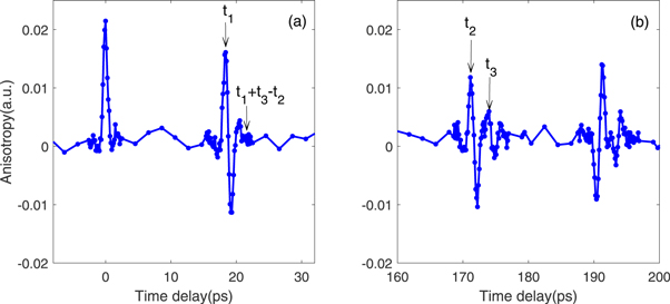
The relative abundance of CH₃ ³⁵Cl and CH₃ ³⁷Cl can be extracted from the relative amplitudes of the anisotropy signal in figure 2(c) at longer times where the two revivals are more separated. However, while the main feature of the revival are separated, there is still some overlap with the smaller features following the revival which need to be considered. Figure 3 shows a close-up of the revivals with index labeled as 0, ½ in figure 3(a), and 4½ and 5 in figure 3(b). The time zero is defined by the peak of 0th revival, and ${t}_{1},\,{t}_{2},\,{t}_{3}$ are time delays of the peak at revival ½, the main peak and minor peak at revival 4½, respectively. While the main peak and minor peak of index 4½ are separated, the anisotropy peak at ${t}_{3}$ is not solely from CH₃ ³⁷Cl as it is affected by the base line of the main peak whose peak is at ${t}_{2}.$ The base line can be estimated by the anisotropy value of revival ½ at ${t}_{1}+{t}_{3}-{t}_{2}$ in figure 3(a) when the revivals from the two isotopologues are almost overlapped in time (timing difference is 0.22 ps).

Zoom In Zoom Out Reset image size

The anisotropy amplitude at ${t}_{3}$ is contributed from two parts; the major portion is from the signal of CH₃ ³⁷Cl, and the other part is from the base line at ${t}_{3}-{t}_{2}$ after the peak at ${t}_{2},$ which is from the signal of CH₃ ³⁵Cl. We use the anisotropy amplitude ${{\rm{Ani}}}_{\exp }({t}_{1}+{t}_{3}-{t}_{2})$ in revival ½ to estimate the contribution from CH₃ ³⁵Cl to the peak at ${t}_{3}$ in revival 4½. We assume the abundance ratio of CH₃ ³⁵Cl to CH₃ ³⁷Cl to be 1: x; thus, the anisotropy contribution from CH₃ ³⁵Cl at ${t}_{3}$ is $\tfrac{1}{x+1}{{\rm{Ani}}}_{\exp }({t}_{1}+{t}_{3}-{t}_{2}).$ The anisotropy amplitude from CH₃ ³⁷Cl at ${t}_{3}$ is ${{\rm{Ani}}}_{\exp }({t}_{3})-\tfrac{1}{x+1}{{\rm{Ani}}}_{\exp }({t}_{1}+{t}_{3}-{t}_{2}),$ and the anisotropy at ${t}_{2}$ from CH₃ ³⁵Cl is ${{\rm{Ani}}}_{\exp }({t}_{2}).$ Therefore, the ratio of the two anisotropy amplitudes is equal to x, and we find the solution x by solving the quadratic equation.

$$\begin{eqnarray}&&\displaystyle \frac{{{\rm{Ani}}}_{\exp }({t}_{3})-\displaystyle \frac{1}{x+1}{{\rm{Ani}}}_{\exp }({t}_{1}+{t}_{3}-{t}_{2})}{{{\rm{Ani}}}_{\exp }({t}_{2})}=x\end{eqnarray} \tag{ 12a }$$

$$\begin{eqnarray}&&x=\displaystyle \frac{{{\rm{Ani}}}_{\exp }({t}_{3})-{{\rm{Ani}}}_{\exp }({t}_{2})+\sqrt{{\left[{{\rm{Ani}}}_{\exp }({t}_{3})-{{\rm{Ani}}}_{\exp }({t}_{2})\right]}^{2}-4{{\rm{Ani}}}_{\exp }({t}_{2})\left[{{\rm{Ani}}}_{\exp }({t}_{1}+{t}_{3}-{t}_{2})-{{\rm{Ani}}}_{\exp }({t}_{3})\right]}}{2{{\rm{Ani}}}_{\exp }({t}_{2})}\end{eqnarray} \tag{ 12b }$$

where Ani_exp(t) is the experimental anisotropy at time t. The measured rotational periods of CH₃ ³⁵Cl and CH₃ ³⁷Cl, the mass difference of the isotopes, and the abundance ratio are calculated and listed in table 1. The experimental values are the average of three independent measurements, and the uncertainty (standard deviation) reflects the range of values retrieved from the three measurements. Based on our measurements, we estimate the uncertainty in the isotope abundance to be 2%, which provides a measure of the sensitivity of the measurement. This value could be improved by increasing the data acquisition time and by recording the data at longer delay times where the revival peaks are better separated. For comparison, the theoretical calculation of rotational periods, isotopic mass difference, and abundance ratio from ref [38–40] are listed as well. The experimental measurements are in good agreement with the theoretical calculations and previous reports.

In summary, we showed that using GUED to probe the rotational dynamics of impulsively aligned molecules, we are able to determine the isotopic composition of a sample of symmetric top gas phase molecules. The rotational period, mass difference, and relative isotope abundance were retrieved from the data on CH₃Cl molecules with ³⁵Cl and ³⁷Cl isotopes. While the method demonstrated here applies only to symmetric top and linear molecules with periodic revivals, we believe the experimental method can in principle be applied to more complex molecules with a suitable modification of the theoretical methods and data analysis. For alignment of asymmetric top molecules, there will be no periodic revivals, however, there is still series of partial revivals that depend on the moments of inertia of the molecule [19]. After measuring the anisotropy experimentally, the measurements could be compared with theoretical calculations of the alignment dynamics for different isotopologues to find the best match between experiment and theory. The main challenge would be that running simulations of rotational dynamics of asymmetric molecules is time consuming, however, it is possible to do using parallel computing.

This work was supported by the National Science Foundation, Physics Division, Atomic, Molecular and Optical Sciences program, under Award No. PHY-1606619.

The data that support the findings of this study are available upon reasonable request from the authors.