
Abstract
We study the dynamics of two charged point particles settling in a Stokes flow.We find what ranges of initial relative positions and what ranges of system parameters lead to formation of stable doublets.The system is parameterized by the ratio of radii, ratio of masses and the ratio of electrostatic to gravitational force.We focus on opposite charges.We find a new class of stationary states with the line of the particle centers inclined with respect to gravity and demonstrate that they are always locallyasymptotically stable. Stability properties of stationary states with the vertical line of the particle centers are also discussed.We find examples of systems with multiple stable stationary states.We show that the basin of attraction for each stable stationary state has infinite measure, so that particles can capture one another even when they are very distant, and even if their charge is very small. This behavior is qualitatively different from the uncharged case where there only exists a bounded set of periodic relative trajectories.We determine the range of ratios of Stokes velocities and ratio masses which give rise to non-overlapping stable stationary states (given the appropriate ratio of electrostatic to gravitational force). For non-overlapping stable inclined or vertical stationary states the larger particle is always above the smaller particle. The non-overlapping stable inclined stationary states existonly if the larger particle has greater Stokes velocity, but there are non-overlapping stable vertical stationary states where the larger particle has higher or lower Stokes velocity.
Export citation and abstract BibTeX RIS

Original content from this work may be used under the terms of the Creative Commons Attribution 4.0 licence. Any further distribution of this work must maintain attribution to the author(s) and the title of the work, journal citation and DOI.
1. Introduction
Motion of particles in a Stokes flow, such as sedimentation, [1–3] has applications including medical technology [4–6], microfluidics [7–11], swimming of microorganisms [12–14], deformation of vesicles [15], waste water treatment [16], marine snow [17], mantle plums [18] and motion within volcanic magma [19, 20]. There are many introductions to the physics of Stokes flows, introduced in [21], such as [22–30] and the included references.
There has recently been interest in bound states of particles in viscous flows. For example, formation of doublets and other bound states of particles in viscous flows have been explored for drops [31], pairs of magnetically active rollers near a repelling wall [32] and for pairs of identical rigid spheres in a background flow with walls [33]. There are also results about large scale spontaneous self-organization into ordered structures with many drops [34] or many rollers [35].
There is also a rich literature in bound states of sedimenting particles. A fundamental problem for the motion of a group of particles close to each other is understanding whether they stay together for a long time or disperse and what are the physical mechanisms responsible for keeping them together, see [36–45]. To make the notion of capturing precise, we define a capturing state of two particles as a configuration whose relative trajectories do not go to infinity in future time. The capturing set is then the set of all capturing states.
In [46] it is shown that there can exist a capturing set of a finite non-zero measure for two uncharged spherical particles of different radii and different masses settling under gravity in a Stokes flow. This set consists of neutrally stable periodic orbits. Because of the neutral stability, there are no basins of attraction, so that even a small perturbation can have a destabilizing effect. Further, because the capturing set has finite measure, if particles begin very distantly they come closer to each other but later move away, and are not trapped. This structure of the capturing set is often used to predict that trajectories of two captured particles are likely to be disturbed by the presence of other particles in a suspension, and therefore capture will probably have no significant effect on the dynamics of sedimenting suspensions e.g., [47–50].
In this paper we study pairs of charged sedimenting particles, in order to see if the charge can create large basins of attraction for bound states. Our interest in electrostatic forces originates from the simple observation that systems of charged particles settling in viscous fluids are common, and therefore stable doublets of charged particles could be potentially used in many practical applications. In a vacuum, electrostatic interactions are destabilizing. This fact is known as Earnshaw's Theorem. However, in [51] it was shown that even a very small charge can stabilize pairs of sedimenting particles; two charged spherical particles of different radii and different masses settling under gravity in a Stokes flow can have locally asymptotically stable stationary states with particle centers in line with gravity.
The stability result in [51] is local. To understand the practical significance of this local result, in this paper we will investigate how two charged point particles sedimenting in a Stokes flow can capture one another, depending on the characteristic parameters of the system: the ratios of the particle radii and masses. We will determine the regions in the phase space of these parameters where stable stationary states of a given interparticle distance can exist. We will determine the capturing set and its structure. We will also find a new class of stable stationary states with particle centers inclined with respect to gravity. We will show that the capturing set of a stable stationary state for two charged point particles settling in a Stokes flow is infinite in measure and consists of one or several basins of attraction to a stable stationary state. These findings open the path toward future experimental observation of these stable doublets. Such doublets could have relevance in dilute charged suspensions [52], for particles in flows at non-zero Reynolds number [53–55] and in plasma [56].
We start our investigation with the mathematical model of point-like particles in section 2. We examine the benchmark case of uncharged pairs of sedimenting point particles (as in [46]) in section 3. In section 4 we present the stability conditions by looking at the linearized dynamics near three kinds of stationary states: centers of particles aligned with gravity with larger particle up, centers of particles aligned with gravity with larger particle down and stationary states where centers of particles are inclined with respect to gravity. In section 5 we discuss generic examples of the relative motion. The vector field of the particle relative velocities and relative trajectories determined numerically on a grid of initial conditions for the case when the larger particle has a greater Stokes velocity. We find the capturing set in physical space of the relative positions using the Poincare-Bendixson theorem. The other case—when the smaller particle has a greater Stokes velocity—is examined in section 6. In section 7 we give the phase diagram for non-overlapping stable stationary states in terms of the ratio of Stokes velocities and ratio of particle radii. We conclude with a summary of our results.
2. Mathematical & physical model
We investigate the dynamics of pairs of charged spherical particles of different radii and masses settling under gravity in a viscous fluid, in the range of the Reynolds number much smaller than unity. A schematic of the system is shown in figure 1. Our goal is to construct the simplest possible analytical model. Therefore, we assume that the particles are point-like and use Coulomb force to model their electrostatic interactions. We also use the point-like model to describe the hydrodynamic interactions. It means that the two-particle mutual mobility is given by the Oseen tensor [26], taken at the relative position of the particles, and self-mobility follows from the Stokes law. The hydrodynamic point-like model is valid when the particles are distant. Further, the electrostatic point-like Coulomb force does not describe effects of, e.g., anisotropic distribution of mobile charges on the particle surface, nor electrostatic screening. Therefore, our approach is an approximation.
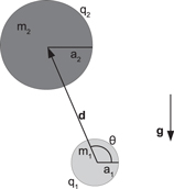
Figure 1. A representation of the geometry of two charged particles with different reduced masses m1 & m2 and radii a1 & a2 settling under gravity in a viscous fluid. The directions of  &
&  are the directions of the gravitational and electrostatic forces respectively. The angle θ of the interparticle position
  from the direction perpendicular to gravity is shown.
Download figure:
Standard image High-resolution imageThe particle pair is labeled so that radius a1 of particle 1 is less than or equal to the radius a2 of particle 2. Via the Stokes equations, we will arrive at equations of motion in terms of the electrostatic and gravitational forces. These are then non-dimensionalized, parameterized and expressed in terms of coordinates.
2.1. Force diagram and dynamics in the point-force approximation
2.1.1. External forces
We start our diagram of forces with gravity. Let  be a unit vector pointing anti-parallel to the constant gravitational field
  . Further, let mi
be the reduced mass of particle i = 1, 2. This means that the particle weight is corrected for the buoyancy force of the fluid. If the fluid has density ρ and the particle has radius ai
and mass Mi
,
. Further, let mi
be the reduced mass of particle i = 1, 2. This means that the particle weight is corrected for the buoyancy force of the fluid. If the fluid has density ρ and the particle has radius ai
and mass Mi
,  . The gravitational force on particle i is

In this paper, we will assume that mi
> 0. The case of mi
≤ 0 can be studied in an analogous way as seen in the supplemental materials of [51]. Now we move on to the electrostatic field. Let  and
and  be the positions of the centers of particle 1 and 2, so that the relative position is

We now move on to the electrostatic forces. We denote the charge on particle i by qi . Then the Coulomb electrostatic force which acts on particle i is

where k is Coulomb's constant and  . The sum of the external forces acting on particle i is

2.1.2. Fluid forces and point force dynamics
We now move on to discuss the fluid forces. We assume that the particles are suspended in an infinite fluid with viscosity μ. We assume that Brownian motion, fluid compressibility and inertia are irrelevant and we describe the fluid flow by the Stokes equations.


where p is the pressure and  is the velocity field of a fluid [22, 23]. Physically, modeling fluid interactions by equations (5) & (6) entails that the external forces on the particles in a Stokes fluid are in balance with the resistance forces exerted on the particles by the fluid so that inertia may be neglected.
In the point particle approximation, the hydrodynamic interactions between the particles are described by a linear dependence of the particle velocities  on the external forces
  acting on them. The mutual interaction is determined by the Oseen tensor [26]

where  is the length of the vector
  ,
,  is the identity tensor and ⨂ is the tensor product. We assume the self-interaction is determined by the Stokes velocity for the particle given by the external forces the particle is experiencing. To sum up, our dynamic equation will be of the form

where  . Notice the above dynamics are first order, which means that the velocities of the particles are given by their positions. This is the mathematical expression of the irrelevance of inertia.
2.2. Characteristic dimensions
In order to aid our analysis we will choose characteristic dimensions. In particular, we choose


as our characteristic length and velocity scale. The time scale is therefore T = L/V. We will use the non-dimensional separation vector

and the time normalized by T to nondimensionalize (8). We further define three independent non-dimensional numbers


which parameterize our equation of motion. One can see that β is the ratio of characteristic electrostatic force to characteristic gravitational force, γ is the ratio of particle radii and δ is the ratio of reduced particle masses. Our assumption that mi > 0 entails that δ > 0 and our labeling convention entails γ ≤ 1. An important physical parameter is also the ratio δ/γ of the particle Stokes velocities.
2.3. Dimensionless equations of motion and their basic properties
Having set up our diagram of forces and nondimensionalization choices, starting from the point-force model (8) we arrive at the following non-dimensional dynamical equation [51]

where dot denotes the non-dimensional time derivative,  and
and  is the non-dimensional Green tensor given by

It is helpful to write equation (15) in terms of coordinates of  . To give a convenient geometry to work in, we will choose x and y axes of the coordinate system so that the particle centers are in the plane y = 0 (the direction of gravity has been already chosen along the z axis). Any orbit with an initial condition in this plane will never experience a force pointing out of this plane, so we will suppress the y-coordinate for the rest of the paper. Using these conventions, equation (15) transformed into Cartesian co-ordinates becomes


A few words can be said about what writing the dynamics in these coordinates entails. First of all, (17) entails that if the particles begin with their centers vertically aligned there are no forces pushing the particles off vertical. This means that, for instance, there is never a periodic orbit which intersects the z-axis. Looking at the signs, we see that (17) is anti-symmetric in αx and αz while (18) is symmetric in αx . Because the dynamics in this coordinate system are given by analytic functions, the pole and the zeros are always isolated points. Further, away from the pole at the origin the dynamics are differentiable, so that orbits never intersect. Finally, the stationary states are given when the LHS of (17) & (18) are both zero, which provides limits on the count of stationary states. When examining the dynamics it is useful to also write the equations in polar co-ordinates and θ the angle from the x-axis. We use polar rather than cylindrical coordinates because there are no forces in the y-direction. These defined so that


where α > 0. This definition entails that the positive x-axis is the ray such that θ = 0, the positive z-axis is  , the negative x-axis is θ = π and the negative z-axis is
  . We could also use
  , the angle from the z-axis. Applying this definition to equation (15), we derive


Writing the dynamics in these coordinates also has a few obvious implications worth making explicit. First of all, the stationary states are given when the LHS of (21) & (22) are both zero. Therefore, equation (22) means that any stationary state must have either  (i.e., the line of the particle centers must be parallel with gravity) or have radial coordinate α equal to

Because α > 0, this second option exists only if

3. Dynamics of uncharged particles
We begin our enumerative strategy by considering the case when at least one particle is uncharged and there is no electrostatic interactions between them. Our analysis will demonstrate the importance of non-stable stationary states in establishing the qualitative global dynamics as well as allow us to discuss later the limit of  . We will also compare the output of this model to the classical results [46].
We start by giving the dynamical equations. If there is at least one uncharged particle, then β = 0 and the equations of motion (21) & (22) become


There are a few trivial cases we will quickly deal with. If δ = 1 then a stationary state only exists if γ = 1 also. In this case, the particles are totally identical and there is no relative motion no matter where the particles begin. Similarly, if δ = γ, either δ = γ = 1 as before or no finite separation can be a stationary state. Either way, this would eliminate any interesting behavior such as bounded orbits. Moreover, only if (24) holds can there be stationary α.
Finally we come to the non-trivial cases, those in which the above inequality is satisfied. Solving for the stationary states gives four solutions: two horizontal and two vertical. The vertical cases haves  or
or  and give

The horizontal cases have  or π and lie at a distance (23) from the origin. A few points can be established about these stationary states just from equations (23) and (27). First we note that
  . Next, if δ > 1, then the right hand side of (27) is an increasing function of γ in our range of 0 < γ ≤ 1. Therefore we have that
  in this case. Stationary states of particles with different radii or different masses can be feasible, i.e., non-overlapping and non-touching, with
  , only if δ < γ < 1.
We illustrate these parameter space results in figure 2(a). The solid line is δ/γ = 1, when the particles have equal Stokes velocities. The short dashed line is equal reduced masses δ = 1. Below this line and above the solid line stationary states do not exist (region D), while above this line stationary states exist but are infeasible (region E). As we have already shown, there is no stationary states on the solid line and short dashed lines except at δ = γ = 1 where every separation is a stationary state.

Figure 2. Dynamics of uncharged particles. (a) Phase space of the ratio γ of particle radii and the ratio δ/γ of the particle Stokes velocities, with the indicated regions defined by equations in table 1. Feasible horizontal and feasible vertical stationary states exist only in region (C). Properties of other regions are given in table 1. (b) Example of relative trajectories for δ = .986 & γ = .988. The orbits of the larger particle, labeled 2, are shown in the reference frame of particle 1, located at the origin. The open circles represent not stable stationary states. The colors are used to facilitate tracing streamlines close to each other.
Download figure:
Standard image High-resolution imageThe dash-dot line is α† = 1, so that above this line but below the solid line (region C) all stationary states are feasible. On the long dashed line is  , so that above this line but below the dash-dot line (region B) vertical stationary states are feasible but the horizontal ones are not feasible. Below dashed line (region A) all stationary states are not feasible. Properties of the regions are outlined in table 1.
Table 1. Properties of stationary states of uncharged particles.
| Region | Do stationary | Are vertical | Are horizontal | |
|---|---|---|---|---|
| states exist? | stationary states | stationary states | ||
| feasible? | feasible? | |||
| (A) |

| yes | no | no |
| (B) |

| yes | yes | no |
| (C) |

| yes | yes | yes |
| (D) |
| no | N/A | N/A |
| (E) |

| yes | no | no |
With the locations of the stationary states in mind, we now turn to characterizing the orbits in the large. We can do this by solving exactly a few special cases of the equations of motion. If our initial condition involves α = α* but θ is non-vertical, then the system evolves along the curve given by


where k1 is from the initial condition. This solution forms two heteroclinic curves, so designated because each connect two stationary states in infinite time.
The other pair of heteroclinic curves are vertical,  or
or  . These heteroclinic are symmetric. In this case the equations of motion are


where k2 is from the initial conditions. This form of the solution makes it clear that a particle approaches θ* in infinite time.
Collectively, the curves sketched out by these four heteroclinic orbits make two half circles. The interior of the curves contain two neutrally stable stationary states at (23). Finally, the two vertical stationary states at (27) are not stable but rather saddle points.
We can now fully characterize the orbit traced out by any initial position. By the Poincare-Bendixson theorem every point on the interior of those closed heteroclinic curves will move in periodic motion: moving toward a stable fixed point is ruled out by linear stability analysis, the heteroclinics have all been found and wandering to infinity is impossible because they cannot touch the closed curves which initially bound them. Finally, every point not vertical and exterior to the circle with radius α* will go to infinity, by similar reasoning.
We complete the analysis by returning to figure 2(a) in order to characterize the qualitative dynamics as a function of the parameters. Regions (A)–(C) & (E) have qualitatively similar dynamics: in all cases there is periodic behavior. Region (D) has no stationary states and therefore all orbits are unbounded. Region (C) has the special property that some of the periodic orbits found are non-overlapping. This case is the most physically interesting and the corresponding relative trajectories are illustrated in figure 2(b). This completes the analysis of the qualitative behavior of uncharged point particles settling in a Stokes flow.
We will now briefly compare the results in this section to those in [46]. This seminal paper uses a precise model of hydrodynamic interactions, allowing for more realistic treatment of finitely sized particles. For reference, figure 2(a) can be compared directly to figure 5 in [46].
The essential similarity between the results of both approaches is that there appear such regions of the phase space γ & δ/γ that all the trajectories are unbounded, and such regions that some of the trajectories are unbounded, but the other ones are bounded. In case of the point-particle model, one should focus on the orbits (or their parts) outside the particle 'surface' determined by its radius. For the point-particle model, region (A) and regions (D) and (E) of figure 2(a) contain only unbounded feasible orbits. Regions (D) and (E), where the larger particle moves slower than the smaller one, are the same as the region of unbounded orbits in [46]. Region (A), in which the larger particle moves faster than the smaller one, is smaller than the region of unbounded orbits in [46].
In the region labeled (C) the feasible point-particle orbits are periodic or unbounded. Analogous (but lager) range was also found in [46] for the more precise hydrodynamic model. In the point-particle region (B) there are feasible unbounded orbits and feasible parts of periodic orbits, bounded owing to the non-overlapping vertical stationary states while the horizontal stationary states responsible for periodicity are overlapping. For the more precise hydrodynamic interactions used in [46], the analogous (but smaller) range exists. However, in this range there are no horizontal stationary states and the bounded orbits are not periodic. Rather, the bounded orbits are heteroclinics going from one vertical stationary state to the other. This comparison suggests that the existence of periodic or bounded orbits is predicted by the point-particle and the more precise hydrodynamic model in a qualitatively similar way when all or at least some of the stationary states are feasible.
4. Linear stability analysis of pairs of charged sedimenting particles
Following the discussion of equation (22), we have divided all the stationary arrangements into three categories. In the first, the particle centers are aligned vertically and the larger particle is above the smaller particle, i.e. θ = π/2 (see figure 1 for illustration). We will call these larger up vertical stationary states. In the second case, the particle centers are also aligned vertically but the larger particle is below the smaller particle, therefore θ = 3π/2. We will call this second configurations larger down vertical stationary states. Finally, there are the inclined stationary states where θ takes on any other value.
The conditions for stability of vertical stationary states were found in [51]. Here we add a systematic analysis of vertical stationary states 1 , both stable and not stable. In this section we also investigate a new class of stationary states: the inclined configurations, focusing on their stability.
4.1. Vertical larger up stationary states
We will first analyze properties of vertical stationary states with the larger particle above the smaller one, i.e. θ = π/2. In this case equation (21) becomes

This equation gives rise to the following condition (equivalent to (14) in [51]) for a stationary state α = α* and 

It follows from this condition that it is possible to choose a β to make any particular α* stationary. Therefore, there are stationary states that have no analogue with the uncharged case. We will return to the parameter space (γ, δ) behavior of vertical stationary states in a later section. For instance, in the range 1 > δ > γ, there are no stationary states for uncharged particles, but there are some if a charge is added. We now address linear stability of a stationary state  , given by equation (33). If we assume that
  and
and  , then the dynamics linear in epsilon are


Because the matrix of coefficients is diagonal, the constants withing the parentheses must be positive in order for the system to be linearly stable. That is,


It can be shown by Lypunov's method that equation (33) and inequalities (36) & (37) form necessary and sufficient conditions for a stationary stable state.
4.2. Vertical larger down stationary states
We will now discuss the stationary states with the larger particle below the smaller one. Similarly to equation (32), on the ray θ = 3π / 2, equation (21) becomes

This gives rise to the following equations for the stationary state 

and for the local dynamics


In order to be linearly stable, the constants within the parentheses must be positive. That is,


We have previously shown in [51] that there are no stable stationary states with the larger particle below the smaller one if we also require the particles do not overlap (α* > 1). However, conditions (42) & (43) will still aid in our understanding of the global dynamics because of the properties of non-stable stationary states.
4.3. Inclined stationary states
In the previous section, we showed how to count and classify the vertical stationary states of charged particles. We will now show how to do the same for non-vertical stationary states, which have a simpler form, given by equations (21), (22) & (23). This simplicity will allow us also to easily analyze typical behaviors in the parameter space (γ, δ).
We can discuss the stationary states of charged particles using figure 2(a) and relations in table 1. The same parameter space curves and regions are of interest but require new interpretations when conceived as relating to charged inclined stationary states. We start from considering two special cases. The short dashed line in figure 2(a) represents equal reduced masses, δ = 1. Equation (22) entails that there exists an inclined stationary state of charged particles only if further δ = γ = 1. Similarly, the solid line, the special case of equal Stokes velocities δ/γ = 1, has an inclined stationary state only if further δ = 1. That is to say, those lines are consistent with the existence of an inclined stationary state only on their intersection point. However, the interpretation of that point is different between the uncharged and the charged inclined case. In the uncharged case, all the relative positions of identical particles are stationary, while in the charged case only stationary states of identical particles must have separation distance  (and an arbitrary orientation). This never feasible distance is the same for all
  . Moving on to the general case of unequal Stokes velocities & unequal reduced masses, a general inclined stationary state must have


Equation (45), identical to (23), corresponds to  . Therefore, the RHS of (45) cannot be negative, and there are no inclined stationary states of charged particles in the region (D) defined in table 1 and shown in figure 2(a). Moreover, the distance between the particles in an inclined stationary state is independent of the charge/mass ratio β. However, unlike the uncharged case, the condition (44) for
  has a nontrivial form that does not allow for stationary states if charges are too large, because the sine of the stationary angle θ† is proportional to charge/mass ratio β. In terms of phase diagram as in figure 2(a), equation (45) entails that all and only values of the parameters γ and δ in region (C), given in table 1 have feasible inclined stationary states of charged particles, providing that value of β is sufficiently small to satisfy (44). Horizontal stationary states, generic for the dynamics of uncharged particles, are exceptional for charged systems. One can see from equation (44) that there is a horizontal stationary state with the particle centers aligned perpendicular to gravity (i.e
  ) if and only if either a) the particles are uncharged (β = 0) or b) the particles have Stokes velocity ratio given by the relation
  (and they overlap with
  ). Because the curve traced by this relation is lower than the dash dot line representing the boundary of feasible inclined stationary states (except at their intersection δ = γ = 1) the angular part of an inclined feasible stable stationary is always less than π, which means that the larger particle is higher than the smaller one.
We now analyze the conditions for linear stability of inclined stationary states. Let  and
and  where
where  r
and θ
are first order perturbations. One finds that to a first order
r
and θ
are first order perturbations. One finds that to a first order


The above linearized dynamics can be easily analyzed. A linear system of ODE with a matrix of constant coefficients is called stable if and only if the real parts of eigenvalues of the matrix are negative. Recall that the determinant is the product of the eigenvalues and the trace is the sum. Therefore, a necessary and sufficient condition for this stationary state to be linearly stable is the determinant to be positive and the trace negative. The determinant

is positive if and only if the particles have different Stokes velocities (recall that  for inclined stationary states),

Further, the trace is equal to

which is negative if and only if

Inequalities (49) & (51) entail that if the charges on the particles are opposed then the stationary states are stable whenever they exist: off of the solid and short dashed line in figure 2(a) and with β small enough that equation (44) has a solution. It is interesting to note that the particles having opposite charges, expressed in the inclined case by inequality (51), is also a necessary condition for a vertical stable steady state [51]. Therefore in the next sections we will focus on systems with oppositely charge particles (i.e. β > 0).
5. Example dynamics of systems of pairs of charged particles
The local information derived in the previous section can be used to find the qualitative behavior of pairs of charged particles sedimenting in a Stokes flow. For instance, as just mentioned, we have shown that the local analysis entails that if there is to be a stable stationary state then the charges on the particles must be opposed. In this section we show some generic examples of the dynamics of charged sedimenting particle doublets with large capturing sets. It means that starting from a wide range of initial relative positions, both particles and will not separate from each other, and, on the contrary, they will decrease their distance for ever.
We choose four sets of parameters to demonstrate a variety of behaviors with the above capturing property. In this section we will choose parameters with β > 0 and δ/γ < 1, so that the particles have opposite charges and the larger particle has greater Stokes velocity when the particles are well separated. The dynamics for when δ/γ > 1 will be discussed in the next section. We organize by the count and arrangement of stable stationary states: one stable vertical stationary state, two stable vertical stationary states, two stable inclined stationary states and finally two stable inclined stationary states with one stable vertical stationary state.
Example orbits solving the nonlinear vector ordinary differential equation (15) are plotted in figure 3. Each orbit describes the relative motion of the larger particle 2 with the origin as the center of the smaller particle 1, and with the given initial relative positions of the larger particle. The orbits were calculated using a fourth order Runga-Kutta method with constant step size Δt = .1. We have decided to use (αx
, αz
) space in this figure and this section for easy comparison with observations. One can see visually that the basins of attraction in our characteristic cases are large. We have also provided in figure 4 a visual way of demonstrating the local stability (or instability) of vertical stationary states. The solid curves are the vertical velocity  of particle 2 relative to particle 1 when their line of centers is vertically aligned and the relative vertical position is αz
. On vertical axis,
of particle 2 relative to particle 1 when their line of centers is vertically aligned and the relative vertical position is αz
. On vertical axis,  which can be obtained from (32) & (38). When the solid curve goes down through the horizontal dash-dot line (which corresponds to
  ) when αz
is increased, then separation between the particle centers is a stationary state which is vertically stable as given by inequalities (36) & (42). The two dashed lines capture the angular stability conditions (37) & (43) for the given parameters, separately for αz
> 0 and αz
< 0. In each of these ranges of αz
, if a stationary state is to the left of a dashed line, then it is horizontally stable. In the following we will demonstrate that using properties of the stationary states we are able to determine basic features of the dynamics and qualitatively describe the boundary of the basin of attraction in all of these generic cases.
) when αz
is increased, then separation between the particle centers is a stationary state which is vertically stable as given by inequalities (36) & (42). The two dashed lines capture the angular stability conditions (37) & (43) for the given parameters, separately for αz
> 0 and αz
< 0. In each of these ranges of αz
, if a stationary state is to the left of a dashed line, then it is horizontally stable. In the following we will demonstrate that using properties of the stationary states we are able to determine basic features of the dynamics and qualitatively describe the boundary of the basin of attraction in all of these generic cases.

Figure 3. These orbits illustrate the relative motion of the larger particle with the origin defined as the center of the smaller particle. The parameters are (a) β = .01, δ = .986 & γ = .988, (b) β = .125, δ = .875 & γ = .885, (c) β = 0.22, δ = 0.45 & γ = 0.5 and (d) β = .42, δ = .47 & γ = .5. The colors are used to facilitate tracing streamlines close to each other.
Download figure:
Standard image High-resolution image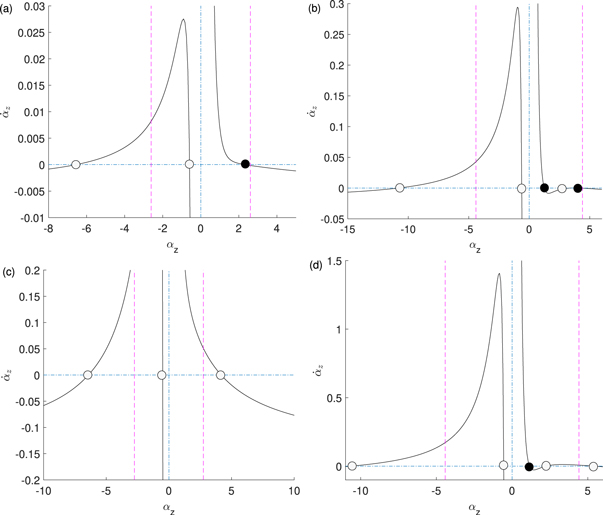
Figure 4. Stability analysis of the vertical stationary configurations shown in figure 3. The dash-dot lines are axes; the horizontal one corresponds to the stationary condition  . The solid curves are the vertical relative velocities
  , evaluated as functions of αz
from (32) & (38). When the solid curve goes down through the horizontal dash-dot line when αz
increases from the stationary position, then that stationary state is vertically stable. In each of the ranges αz
> 0 or αz
< 0, if a stationary state is to the left of a dashed line, given by (37) or (43), then it is horizontally stable.
, evaluated as functions of αz
from (32) & (38). When the solid curve goes down through the horizontal dash-dot line when αz
increases from the stationary position, then that stationary state is vertically stable. In each of the ranges αz
> 0 or αz
< 0, if a stationary state is to the left of a dashed line, given by (37) or (43), then it is horizontally stable.
Download figure:
Standard image High-resolution image5.1. One vertical stable stationary state
We will now apply the results we have derived to find a typical phase portrait of the relative dynamics. As an example, we look at a system with a single stable stationary configuration. We choose the parameters δ = 0.986 & γ = 0.988 from the region (C) and β = 0.01 too large for the existence of inclined stationary states. In this case all of the stationary states have particle centers aligned in the direction of gravity. Relative orbits for different initial positions are illustrated in figure 3(a). It seems that there are two generic classes of orbits visible in this figure, a capturing set and a separating set. In the first one, the particle come closer to each other. In the second one, the particles separate from each other. This informal visual analysis can be deduced by classifying the local behavior of the stationary states and examining the behavior of separatrix and other special orbits. Figure 4(a), which illustrates the behavior of the system when the particle centers are aligned vertically, is helpful for classifying the stationary states. There are three stationary states and a discontinuity at the origin. The stationary state with the larger particle directly above the smaller is αz = 2.31.... This is the sole 'larger up' stationary state. The stationary states with the larger particle directly below the smaller one are αz = −6.56... and αz = −.588.... We will call these the 'far' and 'close' larger down stationary states respectively. We can now classify the stationary states based on their local behavior. Again referring to 4(a), we see the larger up stationary state is stable while the stationary states on the negative z-axis are saddle points. Further, one can see that the far larger down state is stable with respect to horizontal perturbations and unstable with respect to vertical perturbations. Similarly, the close larger down state is unstable with respect to horizontal perturbations and stable with respect to vertical perturbations. Finally, if we briefly and informally consider the origin by considering a point in a punctured neighborhood of the origin we see that it is unstable in the sense that all arrows sufficiently near the origin lead away from the origin.
Now we supplement the local information by considering some special orbits. To simplify language, we will use 'end' to mean the limit in positive infinite time and 'begin' to mean the limit in negative infinite time, taking care to only use this language when it makes sense. There are four special orbits which end on the saddle points. Two vertical special orbits end on the close larger down stationary state: one which begins on the origin and one which begins on the far larger down stationary state.
The most important special orbits, however, are the pair which end on the far larger down stationary state. These non-vertical orbits form the separatrix curve of the system. We use 'separatrix' informally to mean a curve which separates the plane into two sets where the interior and exterior have different qualitative behavior. It is clear to the eye from figure 3(a) that the separatrix cuts the plane into two sets. In fact, the separation property follows from the local information about saddle stationary states.
The separatrix and its interior form the capturing set of the system. In fact, the topology of the vector field shows us a stronger result: all orbits on separatrix or in its interior must go to a stationary state. We start by considering the off vertical orbits on the interior of the separatrix. Such an orbit cannot go to infinity because the orbit cannot cut the separatrix. The orbit cannot be periodic, as a closed orbit in the plane must have a stationary state in its interior—the Poincare-Bendixson theorem—and there are no stationary states off the vertical axis. With periodic motion and separation eliminated, we have shown that all non-vertical orbits on the interior of the separatrix go to a stationary state. Mopping up the remaining special orbits, by examining 4(a) we see the vertical orbits on the interior of the separatrix go to the close larger down stationary state or the stable stationary state. Finally, the orbits that make up the separatrix end on the far larger down stationary state by definition. We have now shown that all orbits in the capturing set go to a stationary state. The demonstration that all orbits in the exterior of the separatrix have the particles drift apart is similar.
This is already a powerful qualitative characterization of the orbits. The local information tells us even more than this. In fact, because any state close to the higher larger down stationary state with non-zero horizontal component is repelled, we see that the vertical special orbits that end on the higher larger down stationary state are the only orbits on the interior of the separatrix which end on the higher larger down stationary state at all. Therefore, almost all points on the interior of the separatrix end on the stable stationary state. This includes, for instance, those orbits on the interior of the curve formed by special orbits which begin on the close larger down stationary state and end on the stable stationary state, which appears as a teardrop shape in figure 3(a).
We have now shown the manner in which the local behavior of the stable and not stable stationary states come together to give us the global dynamics by applying some simple topological reasoning. This completes the description of the qualitative dynamics for this example. We end by again noting that any set of parameters which gives rise to the same structure of stationary states will result in the same qualitative dynamics.
5.2. Two stable vertical stationary states
Similar to the previous example, we can give the global dynamics for when all stationary states are vertical and there are two stable stationary states. As an example of such a system we choose β = .125, δ = .875 & γ = .885. Orbits of particle 2, relative to particle 1, in such a system are illustrated in figure 3 (b). One can see that the capturing set is still large in this case.
In figure 4(b), we plot the relative vertical velocity of the system when the particle centers are aligned vertically, find all vertical stationary configurations and determine their stability against vertical and horizontal perturbations. As before, we can reason from the local information about the stationary states to the global dynamics. The larger up stationary states at αz = 1.242... and αz = 4.130.... are stable. We will call them the near and far stable stationary states, respectively. The stationary state at αz = 3.429... is a saddle point not stable to vertical perturbations, so we will call it the not stable larger up stationary state. Similarly, the two larger down stationary states at αz = − 10.829... and αz = − 0.615... are saddle points and will be called near and far larger down stationary states, respectively.
We shall soon see that all orbits in the capturing set go to a stationary state and furthermore almost all go to a stable steady state. We do this by examining some important orbits and the curves they trace. Once again, the curve made up of orbits which end on the far larger down stationary state is the separatrix that forms the boundary of the capturing set. One can use the argument from the last section to show the separatrix is unbounded. Another important curve is made of the orbits that end in the not stable larger up stationary state. All points on the interior of this curve go to the far stable stationary state and, more obviously, no point on its exterior goes to the far stable stationary state. This curve is also a separatrix, since it is the boundary between basins of attraction of both stable stationary states. It's easy to see that all the orbits off the vertical go to one of these two stable stationary states. From figure 4(b) it is clear that some vertical orbits go to the far larger up stable stationary state, and others go to the near larger down unstable stationary state. This gives us all the qualitative dynamics for systems with two stable vertical stationary states.
5.3. Inclined stable stationary states
We will now examine a characteristic example of dynamics when there are inclined stable stationary states, and they are the only stable stationary states. We choose as our parameters β = 0.22, δ = 0.45 and γ = 0.5. This results in a stable stationary state with α = 2.75..., θ = 0.722... and another one symmetric across the z-axis. One can see by figure 4(c) that these parameters entail there are no vertical stable stationary states. All vertical stationary states are saddle points.
Orbits are illustrated in figure 3(c). Once again, the capturing set is quite large, even though there are no vertical stable stationary states.
We now discuss how the global dynamics is related to the local properties of the stationary states. Once again all orbits in the capturing set go to a stationary state and almost all go to a stable stationary state. However because there are inclined stationary states we must use a new method to show this. Consider pair of orbits that begin on the close larger down saddle point and end on an inclined stable stationary state. These prevent periodic orbits, because any periodic orbit would have to contain an inclined stationary state and therefore cut one of these orbits which is impossible. Further we once more see the boundary of the capturing set is a separatrix coming from infinity and going into the far larger down saddle point. With periodic and unbounded orbits eliminated as possibilities for orbits in the capturing set, the Poincare-Bendixson theorem entails they must all go to some stationary state. The only orbits in the capturing set that do not go to an inclined stationary state are those with initial conditions such that the particle centers are aligned with gravity, which separate the orbits that go to different stable stationary states. We have see again the importance of saddle stationary states in characterizing the qualitative dynamics of particle motion. In this case, the orbits coming out of a saddle point prevented periodic motion. Further, we have repeatedly seen that the seperatrices that form the boundary of the capturing set contain a saddle stationary state. We will see this pattern again in the next case.
5.4. Dynamics with both inclined and vertical stable stationary states
Inclined and vertical stable stationary states can coexist. For example, the parameters β = .42, δ = .47 & γ = .5 have inclined and vertical stationary states. The dynamics of this case can be seen in figure 3(c). We analyze the vertical dynamics in figure 4(d). This example has five vertical and two inclined stationary states. The only vertical stable stationary state has the large particle over the smaller one at αz = 1.15.... The inclined stable stationary states are at α = 4.41.. and θ = 1.15.... The not stable stationary states are the far larger down stationary state at αz = −10.6..., the close larger down stationary state at αz = −.548..., the close larger up stationary state at αz = 2.22.. and the far larger up stationary state at αz = 5.45.... All the not stable stationary states are saddle points.
All orbits in the capturing set go to some stationary state, for the same reason as the previous case. In particular, the orbits coming out of the far larger up stationary state approach the inclined stable stationary states and therefore prevent periodic orbits as seen in figure 3(c). As before, the separatrix which bounds the capturing set is made up of the orbits which end in the far larger down stationary state. The orbits coming from infinity and ending at the the close larger up stationary state form the boundary between the basins of attraction of the inclined and vertical stable stationary states. This completes our analysis of the global dynamics from the local behavior of the stationary states for a system with both stable and inclined stable stationary states.
6. Inverted stokes velocity ratio dynamics
In all the cases of the previous section, when particle separation is large the larger particle moves in the direction of gravity relative to the smaller particle. This is because in all the cases examined the ratio of Stokes Velocities δ / γ < 1. It is also possible to have δ / γ ≥ 1, so that the larger particle moves against gravity relative to the smaller particle when the particle separation is large. We will call this case that of 'inverted Stokes velocity ratio'. The stability considerations from section 4 do not change in form for Inverted Stokes velocity ratios. We will see by example that the Poincare-Bendixson theorem used throughout the previous section still allows us to make qualitative conclusions about the global dynamics.
As our example, we choose parameters β = .293... δ = .82 & γ = .8. This corresponds to the range (D) of the phase space γ & δ/γ, see figure 2(a) and table 1. The corresponding orbits of the larger particle (with the label 2) relative to the smaller particle (with the label 1) are illustrated in figure 5(a). One can see that even though the stable stationary state is still 'larger up' (αz
> 0), the part of the capturing set when the larger particle is above the smaller particle is now bounded, whereas in figure 3 it was not bounded. The part of the capturing set with the larger particle below the smaller particle is now unbounded, whereas before it was bounded. This property of the capturing set corresponds to the inverted direction of the relative trajectories, which have now vertical components coming from  while in the previous section, they arrived from
  , in agreement with the inverted Stokes velocity ratio.
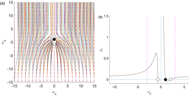
Figure 5. An example system with inverted Stokes velocity ratio δ / γ ≥ 1. One can see from the example orbits in (a) that the larger particle moves against gravity relative to the smaller particle when the separation between them is large. The dynamics when the particle centers are aligned with gravity can be read from (b). The parameters chosen are β = .293... δ = .82 & γ = .8.
Download figure:
Standard image High-resolution imageWe can now extract qualitative information about the dynamics of this system. The dynamics when the particle centers are aligned with gravity are displayed in figure 5(b). The stationary state at  is stable and the stationary states at
  and
and  are saddle points. There are no inclined stable stationary states. The separatrix coming into the larger up saddle point must come in from infinity. This is due to the Poincare-Bendixson theorem: the only other place the separatrix could begin is the larger down saddle point, but this would require a closed curve of orbits without a steady state in the interior. The heteroclinics coming out of the larger down saddle point must go to the stable stationary state. This is also an application of the the Poincare-Bendixson theorem: the orbit cannot diverge without crossing over the heteroclinic coming into the larger up saddle point and cannot be closed because there is no inclined stationary state to be on a closed orbit's interior. Therefore it must end in a stationary state and the only choice is the sole stable one. The curve ending in the larger saddle point is the boundary of the capturing set. Almost all the orbits on the interior of these curves end up on the stable stationary state. All the orbits on its exterior diverge, which corresponds to separation of the particles.
7. Phase diagram for stationary states
In section 3, we gave a phase diagram of the potential stationary states of the pair of uncharged point-particles as a function of the ratio δ/γ of Stokes velocities and the ratio γ of particle radii. Further, in subsection 4.3, we demonstrated how to reinterpret this graph in the case of inclined stationary states of charged particles. In this section we will give the phase diagram appropriate to the case of 'larger up' vertical stationary states, including a heatmap with information about the separation of particle centers at the stable stationary state. We concentrate on such stationary states because we have already shown that 'larger down' vertical stationary states are never stable [51]. We will also compare the phase diagrams and heat maps for vertical and inclined stationary states.
In the remainder of this section we will consider particles of the opposite charges,

because only in this case there exist stable stationary states, as shown in [51]. We will also assume, again following [51], that at the stationary state the particles are non-overlapping (feasible), that is,

This inequality along with equation (33) and inequalities (36) & (37) form necessary and sufficient conditions for a 'larger up' feasible locally asymptotically stable vertical stationary state.
To complete the list of the bounds imposed on the parameters, we remind that

Our goal is to identify the characteristic regions in the parameter space of δ/γ and γ appropriate for feasible vertical 'larger up' stable stationary states of charged point particles, for certain values of β & α*. In fact, we will start by solving equation (33) for β as a function of α*

The conditions (52) and (55) give the following bound on δ/γ as a function of α* and γ,

Because the right hand side of (56) is an increasing function of α*, the greatest lower bound for the ratio of Stokes velocities of oppositely charged particles at a feasible stationary state is reached at α* = 1. This bound is

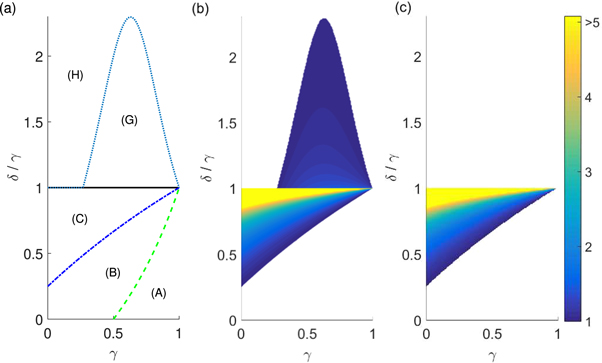
The bound  is plotted by dashed line (green online) in figure 6(a). Below this line, in the range (A), there are no feasible stationary states.
Figure 6. Phase diagrams of stationary states in the parameter space of the ratio of particle radii γ and the ratio of the particle Stokes velocities δ/γ. (a) Non-overlapping 'larger up' stable stationary states exist in regions (C) and (G) but not in (A), (B) and (H). See table 2 for the properties of 'larger up' stationary states in different regions. Vertical and inclined stable stationary states exist in the colored regions of (b) and (c), respectively. Brighter colors correspond to greater values of the maximum distance αmax between the particle centers at the stationary state, as indicated in the color bar.
Download figure:
Standard image High-resolution image
We now analyze angular stability of stationary states. We write inequality (37) as

The minimum of the right hand side, reached at α* = 1, is the greatest lower bound in the phase space (δ/γ, γ) for existence of feasible stationary states stable against angular perturbations,

The bound is plotted by dash-dot line (blue online) in figure 6(a). Below this line, in the range (B), all feasible stationary states are angularly unstable. We now analyze radial stability of stationary states. We use equation (55) to eliminate β from (37). After a careful analysis of signs we obtain

where

It leads to the following least upper bound in the phase space (δ/γ, γ) for existence of stationary states stable against radial perturbations,

where

The bound (62)–(63) is plotted in figure 6(a) as the sum of the boundaries between regions (C) and (H) & regions (G) and (H). Above it, in the range (H), all stationary states are radially unstable.
Basic properties of 'larger up' vertical stationary states in the regions (A)-(H) are outlined in table 2. Recall that the ratio of forces β > 0 has been eliminated using the stationary condition (33) and so remarks about stability should be interpreted with the β so derived. For δ/γ < 1 the requirement of the opposite charges (56) and the angular stability condition (58) give the upper bounds on the interparticle distance at a stationary state,  and
and  , respectively, with

Table 2. Properties of 'larger up' non-overlapping vertical stationary states (each with a certain value of β > 0).
| Region | Properties of stationary states | |
|---|---|---|
| (A) |
 or γ = 1 or γ = 1 | There are no stationary states with  . . |
| (B) |

| For any  there exists a stationary state. There are no stationary states with there exists a stationary state. There are no stationary states with  . Each stationary state is unstable with respect to angular perturbations. . Each stationary state is unstable with respect to angular perturbations. |
| (C) |

| For any  there exists a stationary state. There are no stationary states with there exists a stationary state. There are no stationary states with  . For . For  there exist stable stationary states. For there exist stable stationary states. For  stationary states are angularly unstable. stationary states are angularly unstable. |
| (G) |
 and and 
| For any  there exists a stationary state. Each stationary state is stable against angular perturbations. There exist stable stationary states. there exists a stationary state. Each stationary state is stable against angular perturbations. There exist stable stationary states. |
| (H) |

| For any  there exists a stationary state. Each stationary states is radially unstable and angularly stable. there exists a stationary state. Each stationary states is radially unstable and angularly stable. |
In general, for a given β, γ and δ/γ there might be several stable 'larger up' vertical stationary states with different values of the distance α*. We focus on the largest of them. We find the upper bound on the separation of particle centers, which is graphed in figure 6(b), where the regions of increasingly bright color correspond to regions of increasing separations. The white space corresponds to regions which do not have feasible stable stationary states. Analytically, we choose αmax as the least upper bound of the α* which satisfy inequalities (58) & (60) and we derive the following relation in region (C),

In region (G) this relation is

For comparison, we graph in figure 6(c) the separations of particles for inclined stationary states given by equation (45). As we previously noted, these are feasible only in region (C). One must take care during interpretation because what is plotted in this figure is the exact value rather than merely an upper bound. One can see that for inclined equilbria the lines of constant interparticle separation are monotonically functions of γ, that is that it takes an increasing ratio of Stokes velocities to balance a system with increasing reduced masses at the same separation distance.
8. Conclusions
We have shown that coexistence of hydrodynamic and electrostatic interactions between particles sedimenting in Stokes flows leads to the dynamics essentially different than in the absence of charge or in the absence of fluid. Using the point-particle model, we demonstrated analytically that charged particles can form stable doublets with basins of attraction in the space of the particle relative positions which are very large in comparison to particle radius. This result indicates that charged sedimenting particles can capture one another, even if the initial distance between them is large. The captured particles tend to a certain stable relative position, where the distance between the particle centers is larger than the sum of their radii, so that their surfaces are separated from each other by a fluid. In particular, there exist stable stationary configurations of charged particles separated by large distances, with large basins of attraction, within the range where the hydrodynamic interactions can be approximated as point-like.
Moreover, even if the ratio β of electrostatic to gravitational forces is very small, the dynamics of pairs of charged particles is both quantitatively and qualitatively different from the dynamics in the absence of any electrostatic interactions. The main qualitative difference is the structure of the capturing set in the space of relative positions. For charged particles, the capturing set consists of trajectories tending to a stationary state while for uncharged particles, it consists of neutrally stable periodic orbits.
The existence of a capturing set in the space of the relative positions is associated with the existence of stable stationary configurations of two charged sedimenting particles. However, stable stationary states are formed only for certain ranges of the ratio of particle radii γ and the ratio of Stokes velocities δ/γ. Therefore, we have determined the region in the parameter space of γ and δ/γ where stable stationary configurations exist for certain values of β, and for a certain range of values of the distance α* > 1 between the particles at the stable stationary state. In this way, we have shown that the capturing of charged particles takes place in a large region in the parameter space of γ and δ/γ. Interestingly, for some values of β, γ and δ/γ there exist multiple stable stationary states inside the capturing set.
We have found stable stationary states with the line-of-centers at an angle ψ inclined with respect to gravity. In the point-particle model,  is proportional to the ratio β of electrostatic to gravitational force while the particle-to-particle separation distance α† at the inclined stationary state does not depend on β.
By analyzing examples of capturing sets, we have found that the basin of attraction of all stable stationary states has a boundary which is a surface of revolution of a trajectory which ends on a saddle point stationary state with the particle centers vertically aligned. It seems that the difference between vertical positions of the particles at this stationary state can be used as an estimate of 'the cross-section' of the capturing set. For example, in figure 3(b) and 3(d) the cross section is more than 10 times the sum of the particle radii  , and particle at the stable stationary configuration are separated by more than 4 (a1 + a2). For large capturing sets and large particle separations, the particle dynamics is well-approximated by the point-particle model. Therefore, the analysis presented here suggests that the existence of stable doublets could be confirmed by future experiments.
Acknowledgments
This work was supported in part by the National Science Centre under grant UMO-2018/31/B/ST8/03640.
Data availability statement
All data that support the findings of this study are included within the article (and any supplementary files).
Footnotes
- 1
Though [51] used Cartesian co-ordinates, the resulting stability conditions of vertical stationary states are of course the same as in polar coordinates.