

Abstract
In this paper, we investigate the topological characteristics of the pattern formation in the cooling granular gases confined by the elastic wall. The persistent homology and Voronoi's analysis and its derivative analyses are applied to accomplish our aim. The growth of the pattern formation can be identified by the switch between the logarithmic concave and logarithmic convex in the life-span-distribution obtained using the persistence diagram. Furthermore, three phases are identified by the zeroth or first order Betti number, when a form of the wall is the square. Finally, the characteristics of the coordination of granular particles condensing around the elastic wall are investigated by the Voronoi's analysis, bond-angle analysis, and polyhedral template matching. We confirm that some clusters of the granular particles condensing around the elastic spherical-wall certainly attribute to their crystallization categorized as the typical coordination.
Export citation and abstract BibTeX RIS

Original content from this work may be used under the terms of the Creative Commons Attribution 4.0 licence. Any further distribution of this work must maintain attribution to the author(s) and the title of the work, journal citation and DOI.
1. Introduction
The accurate classification of the phase of matter [1] is significant to characterize the physical property of matter such as solid (crystal structure), liquid, or gases. Meanwhile, such a classification of the phase of matter sometimes involves difficulties as observed in the classification of the phase of glass [2]. For example, we are still unable to answer to the question whether glass corresponds to the liquid, solid or glassy state. The topological characterization of the phase of matter on the basis of locations of atoms or particles has been used in order to overcome such difficulties involved with the specification of the phase of matter. For example, the topological characterization of the crystal has been widely used, as represented by the Voronoi's analysis (VA) using coordination of atoms [3]. On the other hand, the specification of the coordination of atoms (particles) from their locations becomes difficult, when thermal fluctuations of atoms (particles) become significant. Therefore, the specification of the coordination of thermal fluctuating particles involves difficulties even with the VA. Meanwhile, the recent application of the persistent homology (PH) [4] to numerical data (i.e., locations of atoms) of glass by Hiraoka et al [5] succeeded the discrimination of the glassy state from the liquid state, where the coordination of atoms in glass seems to be random, because thermal fluctuations are significant at glance. Then, the PH enables us to find the ordered structure even under the marked thermal fluctuations. The analogy between glass and granular matter is sometimes indicated by the fact that sheared granular media forms the disordered glassy state via the jamming transition [6]. In previous studies of the dense granular packing [7], the characteristics of the force-chain-network was analyzed by the PH, whereas the crystal characteristics of the densely packed granular particles was investigated by the VA.
As a peculiar characteristics of the dilute granular gases, the cluster formation from the initially homogeneous cooling state (HCS) [8, 9] has been well studied by Brey [10] and his coworkers, whereas the characteristics of the HCS of the granular gases has been studied in detail by Santos [11], Brilliantov [8] and their coworkers or Yano [12]. The mode-analysis [8, 10] of the hydrodynamics equation of the granular gases can demonstrate such an instability of the HCS, which attributes to the pattern formation via aggregations (clusters) of the granular particles. Of course, the granular gases correspond to the status, in which the volume fraction of the granular particles is low, adequately, and thermal motions of granular particles are significant. Actually, the phase of granular matter easily changes in accordance with  (ρ: density, L: representative length, rd: diameter of sphere) and restitution coefficient, as demonstrated by Esipov and Pöschel [13]. The primary aim of our present study is to answer to the question whether the transition from the HCS to the pattern formation of the granular gases can be demonstrated by the PH or VA or its derivative analyses, namely, bond-angle analysis (BAA) [14] and polyhedral template matching (PTM) [15]. Additionally, we investigate the crystal structure of granular particles, which condensate around the wall, using the VA, BAA and PTM. Here, the topological phase-transition corresponds to the specific change in topological characteristics, then, we must remind that the topological phase never be same as the physical phase (gases, liquid, or solid).
Now, we consider the granular gases confined by the elastic wall, with which all the granular particles collide elastically. The reason why we consider the elastic (heating) wall [16] is to exclude both excessive accumulation of granular particles around the wall owing to their inelastic collisions with the wall [17] and long range-correlations among granular particles owing to the use of the periodic boundary, which is unfavorable in the PH analysis. The time-evolution of the granular particles with the constant restitution coefficient and smooth surface is calculated by the event-driven (ED) method [17].
This paper is organized as follows. Firstly, the preliminaries for the Betti number [18], persistence diagram (PD) [19], or VA, BAA and PTM are demonstrated together with the ED method in section 2, briefly. Afterwards, the changes in the PD and Betti number in accordance with the time-evolution of the granular particles are discussed in order to confirm whether they are able to capture the transition from the HCS to the pattern formation or not, in section 3. Next, the BAA, VA, and PTM are applied to numerical results of the granular gases confined by the spherical (SP) boundary in order to confirm whether the tendency of the pattern formation of granular gases from the HCS can be identified by the BAA, VA, and PTM or not, in section 4. Additionally, we investigate which coordination the granular particles, which condensate around the elastic wall densely, are categorized as. Finally, we make concluding remarks in section 5.
2. Preliminaries in topological context
Before stating our discussions of numerical results, the following items are demonstrated to help readers' understanding of the mathematical definitions and terminologies used in topological contexts and numerical simulation.
- A.Betti number
- B.Persistence diagram (PD)
- C.From point could data to PD
- D.VA, BAA and PTM
- E.Event Driven (ED) method to simulate granular particles
2.1. Betti number
For a non-negative integer p, the p-th Betti number of simplicial complexes (see its definition in appendix A) is one of classical topological invariants [20]. It is the number assigned to each simplicial complex, which implies information about its topology. The Betti number implies a 'persistence' with respect to 'continuous deformations'. In other words, the Betti number is invariant under 'continuous deformations'. We note that the Betti number does not imply geometric information (volume, metric etc.) of simplicial complexes. Informally speaking, the p-th Betti number of a simplicial complex X is a number of 'p-dimensional holes' of X. We give the heuristic explanation of the Betti number using figure 1. The simplicial complex in figure 1 consists of '7' vertices and '8' edges.

Figure 1. An example of a simplicial complex.
Download figure:
Standard image High-resolution imageA vertex is called as 0-simplex, and an edge is called as 1-simplex from the simplicial point of view. The simplicial complex in figure 1 has no higher-dimensional simplex such as the face. Now, we compute the 0th Betti number. 0-dimensional hole stands for the connected component following conventions. In short, the 0th Betti number counts the number of connected components. Since the simplicial complex in in figure 1 has one connected component, its 0th Betti number is '1'. On the other hand, a 1-dimensional hole means a circular hole. The simplicial complex in figure 1 has two circular holes along with the hexagon part and the square part. Hence, the 1st Betti number is '2'. These observations can be generalized to the case p ≥ 2. For example, we interpret 2-dimensional hole as a balloon-like hole or 2-sphere-like hole. We introduce the notion of homology in order to deal with such 'p-dimensional holes' in a formal way.
Betti number on the basis of locations of granular particles is calculated using the monotone PNG format with the CHomP [21]. Figure 2 shows the zeroth and first order Betti numbers, which are calculated using monotone PNG. We can readily understand that both B0 (connection) and B1 (hole) are equal to '4', as shown in figure 2.

Figure 2. Schematic of calculation of B0 and B1 in 10 × 10 pixels with monotone PNG file by CHomP [21].
Download figure:
Standard image High-resolution image2.2. Persistence diagram (PD)
For a nonnegative integer p, the p-th Betti number counts 'p-dimensional holes' of a simplicial complex, as we explain in section 2.1. A persistence diagram (PD) is a diagram, which records birth and death of 'p-dimensional holes', i.e. we consider 'time-evolution' of a simplicial complex and are interested in the change of its topology.
The time-evolution, formally speaking, corresponds to filtration of a simplicial complex. A filtration of a simplicial complex X is given by a sequence  of simplicial sub-complexes
  parametrized by
  such that
-
 for t0 < t1.
 -
and .


A filtration can be understood as a movie film which records how a simplicial complex grows as time evolves. We give an example in figure 3; the filtration  is an empty complex for sufficiently small t, say t = t−1 ; the filtration
  is constant except for t = t0, t1, t2, where it grows up, as shown in figure 3. The p-th PD of a filtration
  is induced by the data of when the p-dimensional holes are born and dead as time evolves. Informally speaking, for a p-dimensional hole h of some Xt, we mark a point
  on xy-plane where
  (
( , resp.) is the time when the hole h is born (dead, resp.).

Figure 3. An example of a filtration of a simplicial complex.
Download figure:
Standard image High-resolution imageThe p-th PD is obtained by plotting such  . The PD is given by multiple set in general since there is a possibility that some holes have the same birth time and death time. We give an example of the PD in figure 4, which is obtained from the filtration in figure 3. Note that the point
  in the PD has multiplicity of '2'. There is an obvious problem with respect to the definition of such a hole h in the time-evolution. The notion of persistent homology and some decomposition theorems are necessary to define PDs in a formal way. Their brief overview is given in appendix C.
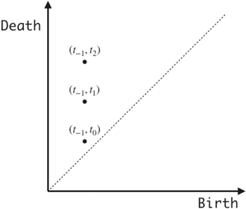
Figure 4. The PD of the filtration in figure 3.
Download figure:
Standard image High-resolution image2.3. From point cloud data to PD
In this subsection, an overview about how the PD is obtained from point cloud data is given. Since the PD is obtained from a filtration of a simplicial complex, it suffices to construct a filtration of a simplicial complex starting from point cloud data. In practice, a point cloud data is usually given by a finite set S in a Euclidean space  . For a positive number
  , an open covering of S in
  given by
  is considered.
Here,  is the
  -neighborhood of a point
  with a radius of
  . There are several ways to construct a cell complex from the open covering
  : the Čech complex, the Alpha complex, the Vietoris-Rips complex, etc [20, 22, 23].
If we denote one of such complexes by  , then,
  gives a filtration of a cell complex where we consider
  as time, i.e.
  for
for  . the PD is obtained from the filtration
  . We note that the PD is determined by the point cloud data S in
  .
.
Figure 5 shows growths of  of eight point cloud by enlarging
  . The upper-left frame of figure 5 shows the birth of the hole, when
  . The upper-middle frame of figure 5 shows births of eight holes, when
  . The upper-right frame of figure 5 shows deaths of holes, when
  . Consequently, the PD of these birth-death-sets of holes
  are shown in lower-frame of figure 5, in which
  and
and  correspond to the radius of
  (i.e.,
  ), which yields the birth and death, respectively. Of course, eight-fold-points are plotted on
  owing to the birth-death of eight holes.
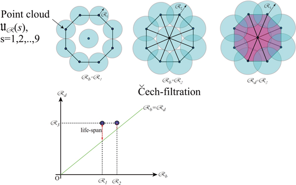
Figure 5.
 of nine point cloud (
 ), when
  (upper-left frame),
  (upper-middle frame) and
  (upper-right frame) in Čech filtration. PD obtained by birth-death of holes corresponding to above three frames (lower frame).
Download figure:
Standard image High-resolution image2.4. VA, BAA and PTM
The Voronoi's analysis (VA), bond-angle-analysis (BAA) and polyhedral template matching (PTM) have been used to analyze the structure of the crystal on the basis of coordination of atoms. In particular, the analytical tools are freely provided by the codes of Voro++ [24] and Vorotop [25] in Ovito [26]. Then, we can utilize such analyzers in order to analyze the crystal structures of granular particles. Of course, the crystal structure usually postulates the densely packed status of granular particles, where thermal fluctuations of atoms are negligible. We, however, focus on the crystal characteristics, before and after granular particles are densely condensed around the wall owing to their markedly low kinetic energy. Here, schematics of the VA, BAA and PTM are demonstrated, briefly.
In order to discuss the VA, BAA and PTM, we start our discussion by mentioning to the Voronoi's diagram (VD).
 is space such as
  (
( ). Let's think elements
  . Here,
  .
.
We define the distance between the point  and
and  as
as

Then, the Voronoi's domain  is defined by:

From equation (1),  is divided into
  (
(![$i\in \left[1,n\right]\cap {\mathbb{N}}$](https://content.cld.iop.org/journals/2399-6528/4/1/015023/revision3/jpcoab6e61ieqn58.gif) ). We call these divided structures of
). We call these divided structures of  by
by  as the VD.
The VD is described by the Delaunay tetrahedralization in the case of  . The significant problem in the VA is classifications of the VD using the typical crystal-coordination such as the face-centered-cubic (FCC), body-centered-cubic (BCC), hexagonal close-packed (HCP), icosahedral (ICO) and hybrid of FCC and HCP (FCC-HCP). The VA by Voro++ applies Weinberg's algorithm [27] to find the most appropriate crystal-coordination among the FCC, BCC, ICO, FCC-HCP and Other from the VD, in which Other indicates the status of coordination of granular particles, from which any crystal structure is not specified with the FCC, BCC, ICO and FCC-HCP.
Of course, there are other methods in order to categorize the crystal structure such as the Common Neighbor Analysis (CNA) [28], PTM [15], BAA [14] other than the VA. The PTM was proposed by Larsen-Schmidt-Schiøtz [15]. In the PTM, the similarity between two diagrams is evaluated by the Root-Mean-Square Deviation (RMSD), which is defined by [15]

where  is the right handed orthogonal matrix ,
  are barycenter of
  and
and  . s is the optimal scaling of
  . The methods of findings of s and
  are proposed by Horn [29] and Theobald [30]. ℵis the number of the neighboring atoms, and
  for the simple cubic (SC), 12 for the FCC, 12 for the HCP, 12 for the icosahedral (ICO) and 14 for the BCC are used. The detail of algorithm of the PTM is demonstrated by Larsen-Schmidt-Schiøtz [15]. Finally, we find the smallest RMSD among them which are calculated using the SC, FCC, HCP, ICO, and BCC. Additionally, Other corresponds to the state that any structure is not identified even with the SC, FCC, HCP, ICO, and BCC, when the minimum RMSD is larger than its critical value. Actually,
  is the vector which indicates the vertex-set of the convex hull formed by N-neighboring atoms and
  is the vector, which indicates the vertex-set of the convex hull of the reference templates, namely, the SC, FCC, HCP, ICO, and BCC (see figure 6 for convex-fulls of the SC, BCC, FCC, HCP and ICO). Hence, we can calculate the distribution of the RMSD (
 : time), when we specify the crystal structure of the atoms using two categories Other and XX (XX := SC, FCC, HCP, ICO and BCC). Finally, we mention to the BAA [14], briefly. The BAA was proposed by Ackland and Jones [14]. The BAA identifies the crystal structure of atom-i with the FCC, HCP, ICO, and BCC from angles (θjik) between two bonds (
 and
and  ), which connect two sets of two neighboring atoms (i-j and i-k). The neighboring atoms are searched by the mean square distance of six neighboring atoms around the atom-i. Once the calculation of the angle between two bonds for several sets of two bonds is finished, functional of χ, which are calculated by angles θjik, identifies the crystal structure of atom-i with the FCC, HCP, ICO, BCC or Other.

Figure 6. Schematic of convex hulls of SC, BCC, FCC, HCP and ICO used in PTM [15].
Download figure:
Standard image High-resolution image2.5. Event-Driven method to simulate granular particles
The event-driven (ED) method has been frequently used in order to simulate a large number (N) of granular particles, whose simulation is difficult using the discrete element method (DEM), when the calculation of the  paired force-chain is beyond the computational resource. In particular, the ED method is suitable to simulate the dilute granular gases, in which the effects of deformations of contacting granular particles on the collective motion of all the granular particles are negligible.
The algorithm of the ED method is so simple. Provided that the k-th collision occurs at t = tk ( ), we search for the occurrence-time of k + 1-th collision, namely, tk+1, which is calculated by

where  is the location of the granular particle indexed by i at
  is the velocity of the i-th granular particle, ri is the radius of the i-th granular particle.
Provided the boundary (wall) is considered, the occurrence-time of the collision between the granular particle and wall is calculated in a similar way to equation (3). Afterward, we compare the next collisional time calculated by two granular particles with that calculated by the granular particle and wall and select smaller tk+1 as next collisional time.
Once tk+1 is determined, we revise the locations of all the granular particles using  (
( ). Finally, we revise the velocities of colliding granular particles or velocity of the granular particle colliding with the wall. Provided that the i-th and j-th granular particles collide, the velocities of colliding granular particles change at t = tk+1 as follows:

where ![$\epsilon \in \left[0,1\right]$](https://content.cld.iop.org/journals/2399-6528/4/1/015023/revision3/jpcoab6e61ieqn80.gif) is the restitution coefficient,
is the restitution coefficient,  is the relative velocity and
  is the relative location-unit-vector.
The calculation of the velocity of the granular particle post-collision with the elastic wall is calculated in a similar way to equation (4) [17].
3. Persistent homology and their characteristics
In this section, we apply the PH to the cooling process of two dimensional granular gases confined by the elastic wall. Firstly, we investigate the PH of the granular discs in the case of the square (SQ) boundary. Next, we investigate the PH in the case of the circular (CI) boundary to consider the effects of form of the elastic wall on the PH. Finally, we investigate the PH of the granular spheres in the case of the spherical (SP) boundary.
3.1. Results in case of SQ boundary
The restitution coefficient of the granular discs is set as  = 0.85, and the volume fraction of the granular discs is fixed as ϕ = 7.85 × 10⁻². The length of one side of the square box (SQ boundary) is set as L = 300. Three types of the diameter of granular discs (rd), namely, rd = 0.15, 0.21 and 0.47 are considered. As a result, total number of granular discs (N) is set as N = 104 in the case of rd = 0.47, N = 5 × 10⁴ in the case of d = 0.21 and N = 105 in the case of rd = 0.15 owing to the constant volume fraction (ϕ = 7.85 × 10⁻²). The initial velocities of the granular discs are randomly distributed in the range of
 ![${v}_{x}\in \left[-1,1\right],{v}_{y}\in \left[-1,1\right]$](https://content.cld.iop.org/journals/2399-6528/4/1/015023/revision3/jpcoab6e61ieqn83.gif) and the initial positions of the granular discs are randomly distributed inside the elastic wall, namely, the range of
and the initial positions of the granular discs are randomly distributed inside the elastic wall, namely, the range of ![$X\in \left[-0.5L,0.5L\right]$](https://content.cld.iop.org/journals/2399-6528/4/1/015023/revision3/jpcoab6e61ieqn84.gif) and
and ![$Y\in \left[-0.5L,0.5L\right]$](https://content.cld.iop.org/journals/2399-6528/4/1/015023/revision3/jpcoab6e61ieqn85.gif) . The time-evolution of granular discs is calculated using the event-driven (ED) method [17], because the conventional molecular dynamics requires the vast calculation time, when forces between
. The time-evolution of granular discs is calculated using the event-driven (ED) method [17], because the conventional molecular dynamics requires the vast calculation time, when forces between  paired granular discs are calculated.
Figures 7–9 show time-evolutions of the granular discs inside the SQ boundary at N = 104, 5 × 10⁴ and 105, respectively. Figure 7 indicates that some clusters are formed in the vicinity of the wall and the cluster with the maximum size rotates to clockwise direction along the wall. Such a rotation of granular discs along the wall is similar to the emergence of the ordered collective-motion in biological swarm inside the wall [31]. On the other hand, the granular particles tend to move away from the wall, when the heating wall with the constant temperature is used, as reported by Esipov and Pöschel [13]. The numerical results obtained using N = 5 × 10⁴ and 105 do not indicate such a rotation of the cluster with the maximum size, as shown in figures 8 and 9. Indeed, it is commonly observed in numerical results of N = 104, 5 × 10⁴ and 105 that the several small-clusters aggregate toward the larger clusters via their connections during the time-evolution. Of course, the elastic wall is a mathematical toy model to avoid the freeze of the calculation via the excessive accumulation of granular discs with the small kinetic energy in the vicinity of the wall and long range correlation of the granular discs owing to the use of the periodic boundary condition, which is unfavorable to topological analyses, because the distance between two granular discs in the PH must be modified by considering the periodicity at the boundary. The calculations of the PDs are performed using locations of the center of granular discs, namely,  (
(![$i\in \left[1,N\right]\cap {\mathbb{N}}$](https://content.cld.iop.org/journals/2399-6528/4/1/015023/revision3/jpcoab6e61ieqn88.gif) ) and
) and  (:radius of neighborhood (cover)
  of point cloud S (
 )). Therefore, we must remind that the connection in d = 0-persistent homology (d: dimension of PH) is not equivalent to the physical connections due to contacting granular discs. Reminding that the domain, which is occupied by neighborhood of i-th point-cloud, whose center is set as
  , is expressed with
  , the connection between
  and
and  is defined by
  (
( ).
).  is increased from zero to
  , continuously in
  .
.  is called as the birth of the hole, when the hole emerges when
  , whereas
  is called as the death of the hole, when the hole disappears, when
  . The plot of
  is called as the PD, as discussed in section 2.2. Additionally,
  is called as the life-span of the hole, and defined by:

The image of the life-span (ℓ) is shown in the lower-frame of figure 5.
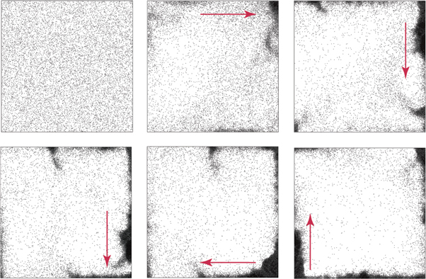
Figure 7. The time-evolutions of granular particles inside SQ boundary at Nc = 0 (upper-left frame),  (upper-middle frame),
  (upper-right frame), 12.5M (lower-left frame), 13.75M (lower-middle frame) and 19.9M (lower-right frame), when N = 104.
Download figure:
Standard image High-resolution image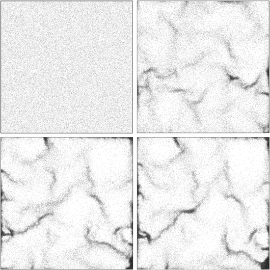
Figure 8. The time-evolutions of granular particles inside SQ boundary at Nc = 0 (upper-left frame), 2M (upper-right frame), 4M (lower-left frame) and 7.4M (lower-right frame), when N = 5 × 10⁴.
Download figure:
Standard image High-resolution image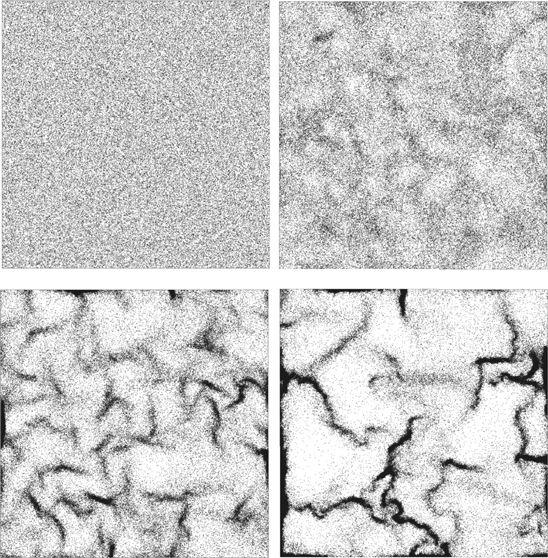
Figure 9. The time-evolutions of granular particles inside SQ boundary at Nc = 0 (upper-left frame), 2.15M (upper-right frame), 3.85M (lower-left frame) and 14.45M (lower-right frame), when  .
.
Download figure:
Standard image High-resolution imageThe open source program homcloud [32] is used to calculate the PD in our study. The PD is plotted using not  but
but  owing to the specification of the homcloud. Figure 10 shows PDs (left-half frames) and birth of holes with
  (maximum value of ℓ) via connections of some of
  (
(![$i\in [1,N]$](https://content.cld.iop.org/journals/2399-6528/4/1/015023/revision3/jpcoab6e61ieqn114.gif) ) at Nc = 0, 2.15M, 3.85M and 11.4M (right-half frames), when N = 105 (Nc: collision number, M: million), respectively. The color of the contour expresses the number of holes, which has
) at Nc = 0, 2.15M, 3.85M and 11.4M (right-half frames), when N = 105 (Nc: collision number, M: million), respectively. The color of the contour expresses the number of holes, which has  , where
  is the square domain, whose center of gravity is
  and length of one side of the square is set as
  . Readers remind that the number of holes which yield
  is unity in all the frames in figure 10. The magnitude of
  obtained using
  increases in accordance with the increase in Nc, as shown in the right-half frame of figure 10, because the growth of clusters of granular discs tends to enlarge the vacant space. The PD has the clear structure at Nc = 0, whereas such a clear structure in the PD becomes blurred at Nc = 14.45M.
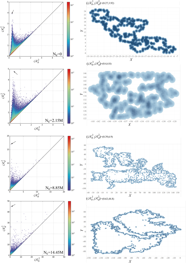
Figure 10. d = 1-PDs and their schematics of births of holes at  in cases of Nc = 0 (top-frame), Nc = 2.15M (2nd frame from the top), Nc = 8.85M (2nd frame from the bottom), and Nc = 14.45M (bottom frame), when N = 105 and SQ boundary. Points, which yield the maximum life-span, are denoted by arrows in each cases of Nc.
Download figure:
Standard image High-resolution imageThe expeditious method to read the characteristics of the PD is to calculate the life-span-distribution (lsd) by each time step. Then, we approximate the lsd, namely,  with
with

where  , and
, and  and m
and m  .
.
The reason why we use equation (6) is that it can express the hybrid of the logarithmic convex (log-convex: for ![$\theta \in [0,1],\theta \mathrm{log}f\left(x\right)+\left(1-\theta \right)\mathrm{log}f\left(y\right)\leqslant \mathrm{log}f\left(\theta x+(1-\theta )y\right)$](https://content.cld.iop.org/journals/2399-6528/4/1/015023/revision3/jpcoab6e61ieqn127.gif) (
( and x < y)) and logarithmic concave (log-concave: for
 ![$\theta \in [0,1],\theta \mathrm{log}f\left(x\right)+\left(1-\theta \right)\mathrm{log}f\left(y\right)\geqslant \mathrm{log}f\left(\theta x+(1-\theta )y\right)$](https://content.cld.iop.org/journals/2399-6528/4/1/015023/revision3/jpcoab6e61ieqn129.gif) (
( and x < y)) using appropriate set of
  in equation (6). Similarly, equation (6) is also able to express completely concave or convex for all the range of ℓ (i.e.,
  ).
).
Figures 11–16 show  versus ℓ together with
  for d = 0 (connection) and 1 (hole) in cases of N = 104, 5 × 10⁴ and 105, whose
  and m in equation (6) are defined in table 1.

Figure 11.
 versus ℓ at Nc = 0 (top-left frame), Nc = 0.25M (top-right frame), Nc = 0.5M (middle-left frame), Nc = 1M (middle-right frame), Nc = 12.5M (middle-left frame), and Nc = 19.9M (middle-right frame) obtained using d = 0, when N = 104 and SQ boundary.
Download figure:
Standard image High-resolution image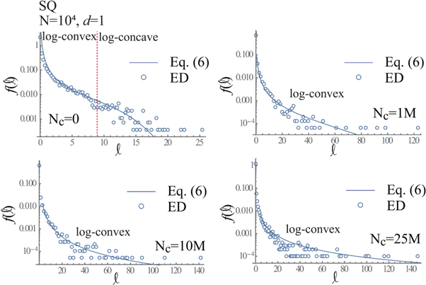
Figure 12.
 versus ℓ at Nc = 0 (upper-left frame), Nc = 1M (upper-right frame), Nc = 10M (lower-left frame) and Nc = 25M (lower-right frame) obtained using d = 1, when N = 104 and SQ boundary.
Download figure:
Standard image High-resolution image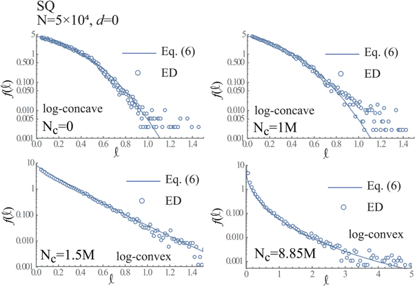
Figure 13.
 versus ℓ at Nc = 0 (upper-left frame), Nc = 1M (upper-right frame), Nc = 1.5M (lower-left frame) and Nc = 8.85M (lower-right frame) obtained using d = 0, when N = 5 × 10⁴ and SQ boundary.
Download figure:
Standard image High-resolution image
Figure 14.
 versus ℓ at Nc = 0 (upper-left frame), Nc = 1M (upper-right frame), Nc = 1.5M (lower-left frame), and Nc = 7.4M (lower-right frame) obtained using d = 1, when N = 5 × 10⁵ and SQ boundary.
Download figure:
Standard image High-resolution image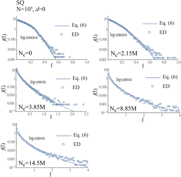
Figure 15.
 versus ℓ at Nc = 0 (upper-left frame), Nc = 2.15M (upper-right frame), Nc = 3.85M (middle-left frame), Nc = 8.85M (middle-right frame), and Nc = 14.5M (bottom-left frame) obtained using d = 0, when N = 105 and SQ boundary.
Download figure:
Standard image High-resolution image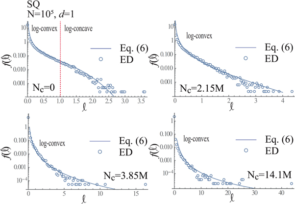
Figure 16. f(ℓ) versus ℓ at Nc = 0 (upper-left frame), Nc = 2.15M (upper-right frame), Nc = 3.85M (lower-left frame) and Nc = 14.1M (lower-right frame) obtained using d = 1 when N = 105.
Download figure:
Standard image High-resolution imageTable 1.
 and m in equation (6) and corresponding figure number, when d = 0 and 1, N = 104, 5 × 10⁴ and 105, and SQ boundary are used.
| Form | d | N | Nc |

|

|

|

|

|
n | m | Figure No. |
|---|---|---|---|---|---|---|---|---|---|---|---|
| SQ | 0 | 104 | 0 | 0.8 | 0.29 | 0 | 1 | 1 | 2 | 0.2 | Figure 11 |
| SQ | 0 | 104 | 2.5M | 1.2 | 0.29 | 0 | 1 | 1 | 1.8 | 0.35 | Figure 11 |
| SQ | 0 | 104 | 5M | 2.25 | 0.15 | 0 | 1 | 1 | 0.8 | −2.5 | Figure 11 |
| SQ | 0 | 104 | 12.5M | 0.25 | 0.05 | 0 | 1 | 0.1 | 1.26 | −1.5 | Figure 11 |
| SQ | 0 | 104 | 19.9M | 0.15 | 0.03 | 0 | 1 | 1 | 1.26 | −1.5 | Figure 11 |
| SQ | 0 | 5 × 10⁴ | 0 | 4.5 | 5.5 | 0 | 1 | 1 | 2.2 | −2 | Figure 13 |
| SQ | 0 | 5 × 10⁴ | 1M | 4.5 | 5.5 | 0 | 1 | 1 | 2.2 | −2 | Figure 13 |
| SQ | 0 | 5 × 10⁴ | 1.5M | 8 | 3.25 | 0 | 1 | 1 | 1 | −3 | Figure 13 |
| SQ | 0 | 5 × 10⁴ | 8.85M | 12 | 3.25 | 0 | 1 | 1 | 0.25 | −3 | Figure 13 |
| SQ | 0 | 105 | 0 | 10 | 25 | 0 | 1 | 1 | 2 | −3 | Figure 15 |
| SQ | 0 | 105 | 2.15M | 10 | 15 | 0 | 1 | 1 | 1.7 | −3 | Figure 15 |
| SQ | 0 | 105 | 3.85M | 8 | 4.2 | 0 | 1 | 0.75 | 0.5 | −5 | Figure 15 |
| SQ | 0 | 105 | 8.85M | 0.5 | 0.1 | 0 | 1 | 0.75 | 1.2 | −5 | Figure 15 |
| SQ | 0 | 105 | 14.5M | 0.5 | 0.1 | 0 | 1 | 0.75 | 1.2 | −5 | Figure 15 |
| SQ | 1 | 104 | 0 | 0.003 | 2.5 × 10⁻⁵ | 0 | 0.067 | 10−5 | 4 | −1.5 | Figure 12 |
| SQ | 1 | 104 | 1M | 0.005 | 6.1 × 10⁻⁹ | 0 | 0.2 | 10−5 | 2 | −1.5 | Figure 12 |
| SQ | 1 | 104 | 5M | 0.005 | 2.2 × 10⁻¹⁰ | 0 | 0.2 | 10−5 | 3.2 | −1.75 | Figure 12 |
| SQ | 1 | 104 | 12.5M | 0.005 | 3.57 × 10⁻²² | 0 | 0.2 | 10−5 | 6.2 | −1.35 | Figure 12 |
| SQ | 1 | 5 × 10⁴ | 0 | 5 × 10⁻³ | 3.14 × 10⁻² | 0 | 0.2 | 10−5 | 3 | −1.5 | Figure 14 |
| SQ | 1 | 5 × 10⁴ | 1M | 5 × 10⁻³ | 1.6 × 10⁻² | 0 | 0.2 | 10−5 | 3 | −1.5 | Figure 14 |
| SQ | 1 | 5 × 10⁴ | 1.5M | 5 × 10⁻³ | 0.136 | 0 | 0.2 | 10−5 | 1.5 | −1.75 | Figure 14 |
| SQ | 1 | 5 × 10⁴ | 7.4M | 1.2 × 10⁻³ | 3.79 × 10⁻³ | 0 | 0.2 | 10−5 | 0.98 | −2.4 | Figure 14 |
| SQ | 1 | 105 | 0 | 5 × 10⁻³ | 0.25 | 0 | 0.5 | 0 | 3 | −1.5 | Figure 16 |
| SQ | 1 | 105 | 2.15M | 0.02 | 1 | 0 | 0.4 | 0 | 1 | −1.5 | Figure 16 |
| SQ | 1 | 105 | 3.85M | 0.01 | 0.71 | 0 | 0.4 | 0 | 0.5 | −2 | Figure 16 |
| SQ | 1 | 105 | 14.5M | 0.01 | 1 | 0 | 0.4 | 0 | 1.5 × 10⁻³ | −2.5 | Figure 16 |
The authors will consider that one standard for the evaluation of the topological phase-transition of the granular discs is determined by the switch between the log-convex and log-concave of  (or
(or  ), as discussed later. Figure 11 indicates that
  (or
(or  ) follows the log-concave at Nc = 0 and 0.25M, whereas
  (or
(or  ) follows the log-convex at 0.5M≤ Nc. Consequently, we conclude that the topological phase-transition occurs in the range of 0.25M< Nc < 0.5M, when d = 0 and N = 104. Similarly, figure 12 indicates that
  (or
(or  ) follows the log-convex at
  and log-concave at
  in the case of Nc = 0, whereas
  (or
(or  ) follows the log-convex at 0 ≤ ℓ. As a result, the topological phase-transition occurs in the range of Nc ∈ [0, 1M], when d = 1 and N = 104. These topological phase-transitions are obtained at Nc ∈ [1M,1.5M] in both cases of d = 0 and 1, when N = 5 × 10⁴, as shown in figures 13 and 14, whereas it is obtained at Nc ∈ [2.15M,3.85M] in both cases of d = 0 and 1, when N = 105, as shown in figures 15 and 16.
The lsd obtained using d = 1-PD, which follows the log-convex, indicates that the number of holes with the large diameter  and small
  (i.e., long life-span) is larger than that obtained using the d = 1-PD, which follows the log-concave. The holes with the long life-span are generated by the increase of vacant space and connections of point-clouds by small
  , which are caused by the growths of clusters. Consequently, the switch between the log-concave and log-convex becomes the standard to measure the drastic growth of clusters, by which the topological characteristics of granular gases changes, markedly.
From above discussions, we confirmed that the topological phase-transition can be judged by the switch of the life-span-distribution (lsd) (i.e.,  ) between the log-convex and log-concave. Here, we investigate the topological phase-transition using the Betti number, B0 (the zeroth order) and B1 (the first order). As discussed in section 2, the Betti number is calculated using the PNG versions of figures 7–9. Therefore, the accuracies of the calculations of B0 and B1 depend on the number of pixels in PNG versions of figures 7–9. Figure 17 shows B0/N and B1/N in cases of N = 104 (upper-left frame), 5 × 10⁴ (upper-right frame) and N = 105 (lower-left frame). B0/N ≃ 0.96 at Nc = 0 obtained using N = 105 indicates that the numerical error exists owing to the insufficient number of pixels, whereas B0/N = 1 at Nc = 0 obtained using N = 104 and 5 × 10⁴ indicate that the number of pixels is adequate to calculate B0 and B1 with the good accuracy.

Figure 17. B0 and B1 versus Nc, when  (upper-left frame), 5 × 10⁴ (upper-right frame) and 105 (lower-left frame).
Download figure:
Standard image High-resolution imageFirstly, we confirm that there exist typical three phases (i.e., phases-I, II and III) in cases of N = 5 × 10⁴ and 105. In the phase-I, B0 (B1) decreases (increases), drastically, as shown in Nc ∈ [0,0.5M] when N = 5 × 10⁴, and Nc ∈ [0,1M] when N = 105. In the phase-II, B0 (B1) changes, slightly, as shown in Nc ∈ [0.5M,1.5M] when N = 5 × 10⁴ and Nc ∈ [1M,2M] when N = 105. Finally, in the phase-III, B0 (B1) decreases (increases), drastically, as shown in Nc ∈ [1.5M,  ) when N = 5 × 10⁴ and Nc ∈ [2M,
  ) when N = 105. We are, however, unable to identify phases-I and II, clearly, when N = 104, whereas the phase-III is conformed in Nc ∈ [0.25M,
  , when N = 104. The increase and decrease in B0 and B1 in the phase-III are caused by temporal changes in form of rotating cluster along the wall obtained using N = 104, so that such changes in phase-III do not attribute to intrinsic changes in the topological phase, which characterize the pattern formation from the HCS. It is the significant result that the topological phase-transition from the phase-I to the phase-II is identified by not the lsd but B0 and B1, whereas the phase-transition due to the topological phase-transition from the phase-II to the phase-III is identified by both the lsd and B0 and B1.
3.2. Results in case of CI boundary
Now, we investigate the PH in the case of the CI boundary in order to investigate the effects of form of the elastic wall on the PH. The radius of the granular disc (rd) is set as rd = 0.15 and radius of the CI (Rd) is set as Rd = 150. The set of the restitution coefficient and initial velocities of the granular discs are same as those used in calculations in the case of the SQ boundary. The total number of the granular discs (N) is set as  . As a result, the volume fraction of granular discs (ϕ) is calculated as ϕ = 0.1, because all the granular discs are randomly distributed inside the CI boundary at t = 0.
Figure 18 shows snap-shots of the granular discs confined by the CI boundary at Nc = 0 (upper-left frame), Nc = 2.5M (upper-center frame), Nc = 5M (upper-right frame), Nc = 7.5M (lower-left frame), Nc = 15M (lower-center frame) and Nc = 35M (lower-right frame). We can confirm the clear pattern formation at 5M≤Nc. In particular, the clusters seem to grow from the wall at Nc = 35M.

Figure 18. Snap-shots of granular discs confined by CI boundary at Nc = 0 (upper-left frame),  (upper-center frame), Nc = 5M (upper-right frame), Nc = 7.5M (lower-left frame), Nc = 15M (lower-center frame) and Nc = 35M (lower-right frame).
Download figure:
Standard image High-resolution imageFigure 19 shows the d = 1-PDs at Nc = 0 (top-left frame), Nc = 2.5M (top-right frame), Nc = 5M (middle-left frame), Nc = 7.5M (middle-right frame), Nc = 15M (bottom-left frame) and Nc = 35M (bottom-right frame), when Nc = 105 and CI boundary. The tendency of changes in the d = 1-PD during the time-evolution is similar to that obtained using the SQ boundary in figure 10. Figures 20 and 21 show  versus ℓ together with
  (in equation (6)) versus ℓ when d = 0 and d = 1, respectively, where
  and m in equation (6) are defined in table 2. We can confirm that the topological phase-transition occurs in Nc ∈ [2.5M,5M] in both cases of d = 0 and 1, as shown in figures 20 and 21.
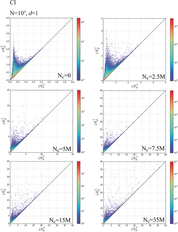
Figure 19. PD obtained using d = 1 at Nc = 0 (top-left frame), Nc = 2.5M (top-right frame), Nc = 5M (middle-left frame), Nc = 7.5M (middle-right frame), Nc = 15M (bottom-left frame) and Nc = 35M (bottom-right frame), when Nc = 105 and CI-boundary.
Download figure:
Standard image High-resolution image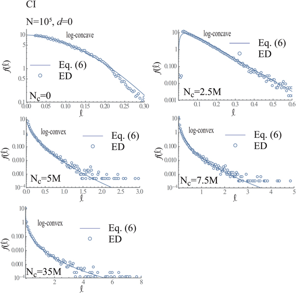
Figure 20.
 versus ℓ at Nc = 0 (top-left frame),
  (top-right frame), Nc = 5M (middle-left frame), Nc = 7.5M (middle-right frame) and Nc = 35M (bottom-left frame) obtained using d = 0, when N = 105 and CI boundary.
Download figure:
Standard image High-resolution image
Figure 21.
 versus ℓ at Nc = 0 (upper-left frame), Nc = 2.5M (upper-right frame), Nc = 5M (lower-left frame), and Nc = 35M (lower-right frame) obtained using d = 1, when N = 105 and CI boundary.
Download figure:
Standard image High-resolution imageTable 2.
 and m in equation (6) and corresponding figure number, when d = 0 and 1, N = 105 and CI boundary are used.
| Form | d | N | Nc |

|

|

|

|

|
n | m | figure No. |
|---|---|---|---|---|---|---|---|---|---|---|---|
| CI | 0 | 105 | 0 | 1 | 34.8 | 0 | 1 | 3.15 | 1.74 | 2 | Figure 20 |
| CI | 0 | 105 | 2.5M | 900 | 18 | 0 | 1 | −10−4 | 0.8 | 1 | Figure 20 |
| CI | 0 | 105 | 5M | 100 | 9.5 | 0 | 1 | −10−4 | 0.48 | 0.35 | Figure 20 |
| CI | 0 | 105 | 7.5M | 50 | 8 | 0 | 1 | −10−4 | 0.4 | 0.2 | Figure 20 |
| CI | 0 | 105 | 35M | 50 | 8 | 0 | 1 | −10−4 | 0.3 | 0.15 | Figure 20 |
| CI | 1 | 105 | 0 | 0.05 | 0.75 | 0 | 1 | 10−7 | 3 | −1.4 | Figure 21 |
| CI | 1 | 105 | 2.5M | 0.05 | 0.75 | 0 | 1 | 10−7 | 2 | −1.4 | Figure 21 |
| CI | 1 | 105 | 5M | 0.02 | 0.15 | 0 | 1 | 10−7 | 1.2 | −1.75 | Figure 21 |
| CI | 1 | 105 | 35M | 0.02 | 0.15 | 0 | 1 | 10−7 | 1.2 | −1.75 | Figure 21 |
Figure 22 shows B0/N, B1/N and  . Similarly to B0/N obtained using N = 105 and the SQ boundary, B0/N ≃ 0.96 indicates that the numerical error exists owing to the insufficient number of pixels. We can readily confirm that phases-II and III exist in Nc ∈ [0,2M] and Nc ∈ [2M,
  ). It is not obvious in the present study whether the lack of the phase-I in the case of the CI boundary is caused by the different form of boundary from the SQ boundary or larger volume fraction (ϕ = 0.1) in CI boundary than that (ϕ = 0.078 5) in the SQ boundary. The phase-transition due to the topological phase-transition from the phase-II to the phase-III is obtained using both the lsd and Betti number in the case of the CI boundary.
3.3. Results in case of SP boundary
Next, we investigate the PH in the case of the SP boundary. As discussed in section 2, the 3D physical space postulates the PH with d = 2, which corresponds to the spherical surface (void). Here, we consider two types of N. In one case, N = 5 × 10⁴ granular spheres with rd = 1.5 are calculated. In the other case, N = 104 granular spheres with rd = 1.5 are calculated. In both cases, the radius of the SP boundary is set as Rd = 150 and restitution coefficient is set as 0.85. Consequently, the volume fraction is 5% in the case of N = 5 × 10⁴ and 1% in the case of N = 104, because all the granular spheres are randomly (almost homogeneously) distributed inside the SP boundary. The restitution coefficient of the granular spheres is set as 0.85 and the initial velocities of granular spheres are randomly selected in the ranges of ![${v}_{x}\in [-1,1],{v}_{y}\in [-1,1]$](https://content.cld.iop.org/journals/2399-6528/4/1/015023/revision3/jpcoab6e61ieqn183.gif) and
and ![${v}_{z}\in [-1,1]$](https://content.cld.iop.org/journals/2399-6528/4/1/015023/revision3/jpcoab6e61ieqn184.gif) .
.
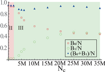
Figure 22. B0/N, B1/N and  versus Nc obtained using CI boundary.
Download figure:
Standard image High-resolution imageFigure 23 shows the snapshots of the granular spheres confined by the SP boundary, when N = 104 (upper two raw) and N = 5 × 10⁴ (lower two raw). The granular spheres cluster in the vicinity of the SP boundary with the band-like form as Nc increases, when N = 104,. On the other hand, some band-like distributions of granular spheres emerge along the SP boundary in accordance with the increase in Nc when N = 5 × 10⁴. The aggregation of granular spheres in the vicinity of the wall at large Nc is similar to those in 2D cases of the SQ and CI boundaries.
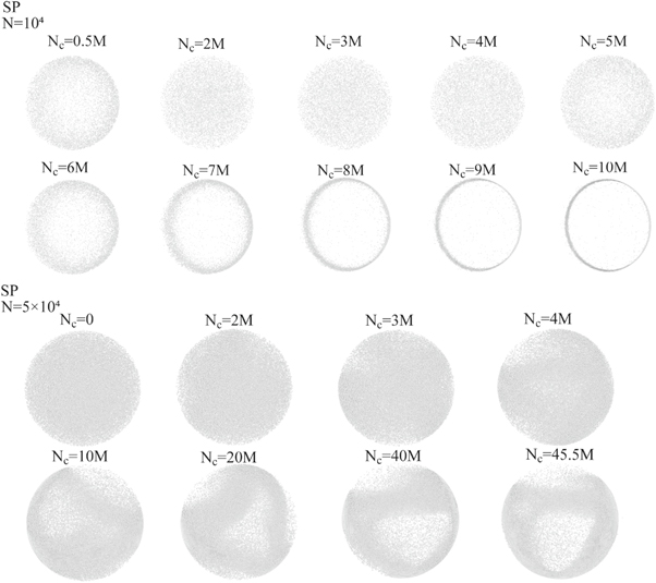
Figure 23. Snapshots of granular spheres confined by SP boundary at each Nc when N = 104 (upper two raw) and 5 × 10⁴ (lower two raw).
Download figure:
Standard image High-resolution imageFigures 24–27 show time-evolutions of d = 1-PDs and d = 2-PDs obtained using Nc = 104 and 5 × 10⁴, respectively. The tendency of temporal changes in d = 1-PDs is similar to those obtained using the SQ and CI boundaries. d = 2-PDs obtained using N = 104 indicate that the life-spans of most of granular spheres approach to zero at Nc = 5.5M, when N = 104, although the life-spans of some of granular spheres are finite, as observed in d = 1-PD at Nc = 5.5M in figure 24. Meanwhile, the life-spans of granular spheres observed in d = 2-PDs are finite at Nc = 40M, when N = 5 × 10⁴, as shown in figure 27.
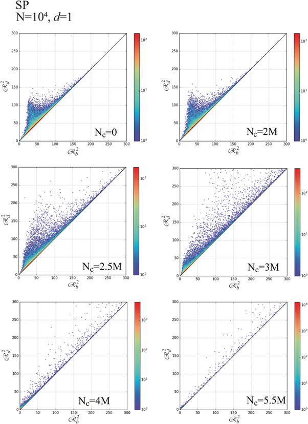
Figure 24. PD obtained using d = 1 at Nc = 0 (top-left frame), Nc = 2M (top-right frame), Nc = 2.5M (middle-left frame), Nc = 3M (middle-right frame), Nc = 4M (bottom-left frame) and Nc = 5.5M (bottom-right frame), when Nc = 104 and SP-boundary.
Download figure:
Standard image High-resolution image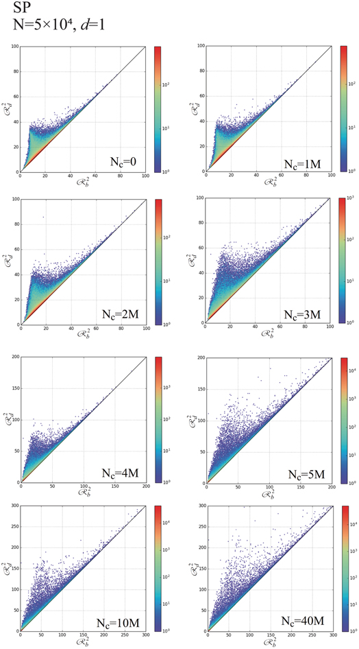
Figure 25. PD obtained using d = 1 at Nc = 0 (top-left frame),  (top-right frame), Nc = 2M (second top-left frame), Nc = 3M (second-right frame), Nc = 4M (second bottom-left frame), Nc = 5M (second bottom-right frame), Nc = 10M (bottom-left frame), Nc = 40M (bottom-right frame), when Nc = 5 × 10⁴ and SP-boundary.
Download figure:
Standard image High-resolution image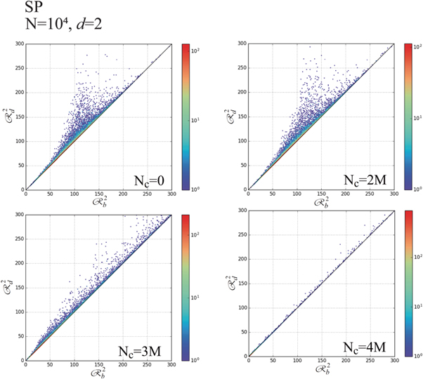
Figure 26. PD obtained using d = 2 at Nc = 0 (upper-left frame),  (upper-right frame), Nc = 3M (lower-left frame), and Nc = 4M (lower-right frame), when Nc = 104 and SP-boundary.
Download figure:
Standard image High-resolution image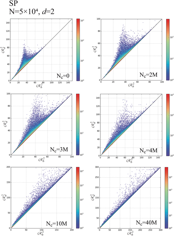
Figure 27. PD obtained using d = 2 at Nc = 0 (top-left frame), Nc = 2M (top-right frame), Nc = 3M (middle-left frame), Nc = 4M (middle-right frame), Nc = 10M (bottom-left frame), Nc = 40M (bottom-right frame), when Nc = 5 × 10⁴ and SP-boundary.
Download figure:
Standard image High-resolution imageFigures 28–33 show  versus ℓ together with
  versus ℓ obtained using N = 104 and 5 × 10⁴, when d = 0, 1 and 2, respectively, where
  and m in equation (6) are defined in table 3. Figures 28 and 30 indicate that the topological phase-transition occurs in Nc ∈ [2M,2.5M] in the case of N = 104, whereas all of
  for d = 2 follow log-convex at Nc ∈ [0,
  ), when N = 104, as shown in figure 32. Similarly, the topological phase-transition occurs in Nc ∈[3M,4M], when N = 5 × 10⁴, as shown in figure 29. The log-concave of f(ℓ) remains at Nc = 45M, when d = 1 and N = 5 × 10⁴, as shown in figure 31. Then, we cannot determine the topological phase-transition from the lsd for d = 1, when N = 5 × 10⁴. Similarly to f(ℓ) obtained using d = 2 and N = 104, all of
  follow the log-convex in
  , as shown in figure 33. Consequently, we conclude that the lsd for d = 2 can not be used as the standard, which determines the topological phase-transition in accordance with the switch of the lsd between the log-concave and log-convex in both cases of N = 104 and 5 × 10⁵.
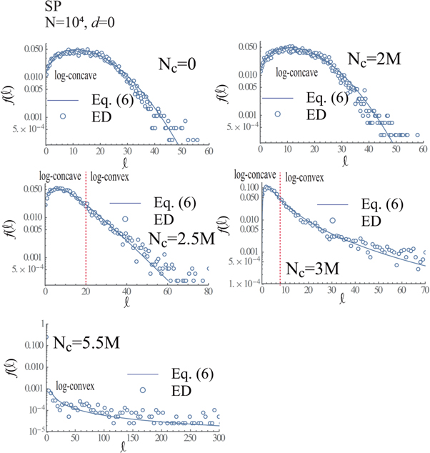
Figure 28.
 versus ℓ at Nc = 0 (top-left frame),
  (top-right frame), Nc = 2.5M (middle-left frame), Nc = 3M (middle-right frame) and Nc = 5.5M (bottom-left frame) obtained using d = 0, when N = 104 and SP boundary.
Download figure:
Standard image High-resolution image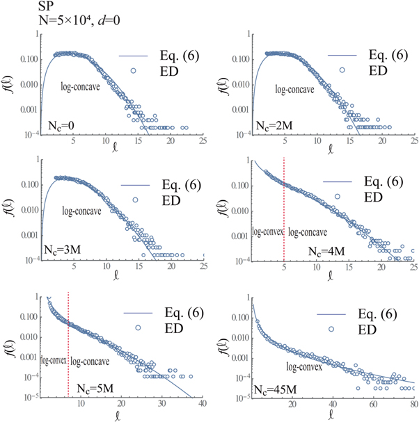
Figure 29.
 versus ℓ at Nc = 0 (top-left frame), Nc = 2M (top-right frame), Nc = 3M (middle-left frame), Nc = 4M (middle-right frame), Nc = 5M (bottom-left frame) and Nc = 45M obtained using d = 0, when N = 5 × 10⁴ and SP boundary.
Download figure:
Standard image High-resolution image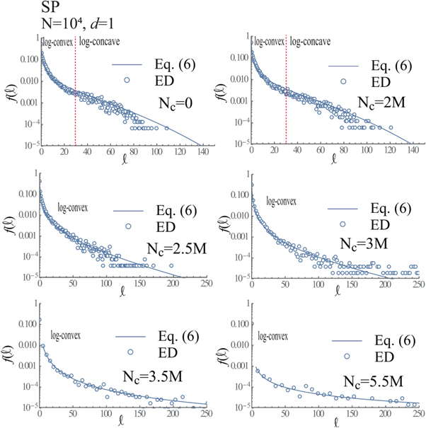
Figure 30.
 versus ℓ at Nc = 0 (top-left frame), Nc = 2M (top-right frame), Nc = 2.5M (middle-left frame), Nc = 3M (middle-right frame), Nc = 3.5M (bottom-left frame) and Nc = 5.5M obtained using d = 1, when N = 104 and SP boundary.
Download figure:
Standard image High-resolution image
Figure 31.
 versus ℓ at Nc = 0 (top-left frame), Nc = 2M (top-right frame), Nc = 3M (middle-left frame), Nc = 4M (middle-right frame), Nc = 5M (bottom-left frame) and Nc = 45M obtained using d = 1, when N = 5 × 10⁴ and SP boundary.
Download figure:
Standard image High-resolution image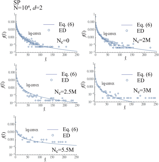
Figure 32.
 versus ℓ at Nc = 0 (top-left frame), Nc = 2M (top-right frame), Nc = 2.5M (middle-left frame), Nc = 3M (middle-right frame) and Nc = 5.5M (bottom-left frame) obtained using d = 2, when N = 104 and SP boundary.
Download figure:
Standard image High-resolution image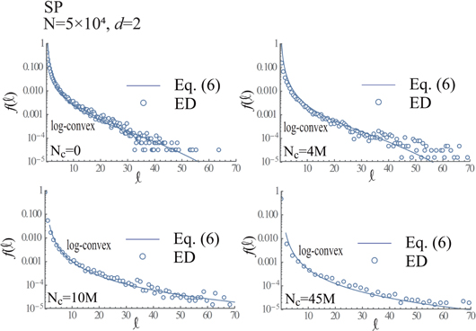
Figure 33.
 versus ℓ at Nc = 0 (upper-left frame), Nc = 4M (upper-right frame), Nc = 10M (lower-left frame) and Nc = 45M (lower-right frame) obtained using d = 2, when N = 5 × 10⁴ and SP boundary.
Download figure:
Standard image High-resolution imageTable 3.
 and m in equation (6) and corresponding number of the figure, when d = 0, 1 and 2, N = 104 and 5 × 10⁴ and SP boundary are used.
| Form | d | N | Nc |

|

|

|

|

|
n | m | figure No. |
|---|---|---|---|---|---|---|---|---|---|---|---|
| SP | 0 | 104 | 0 | 0.012 | 0.003 | 1 | 0.8 | 1 | 2 | 0.75 | Figure 28 |
| SP | 0 | 104 | 2M | 0.012 | 0.003 | 1 | 0.8 | 1 | 2 | 0.75 | Figure 28 |
| SP | 0 | 104 | 2.5M | 0.02 | 0.003 | 1 | 0.8 | 1 | 0.95 | 1 | Figure 28 |
| SP | 0 | 104 | 3M | 5 × 10⁷ | 18 | −1 | 1 | 0 | 2 | 0.15 | Figure 28 |
| SP | 0 | 104 | 5.5M | 1 | 0 | 0 | 1 | −614 | 1 | 0.77 | Figure 28 |
| SP | 1 | 104 | 0 | 1 | 2.25 × 10⁻⁴ | 0 | 3.6 | 1.83 | 2 | −1.15 | Figure 30 |
| SP | 1 | 104 | 2M | 1 |

|
0 | 3.6 | 1.83 | 2 | −1.15 | Figure 30 |
| SP | 1 | 104 | 2.5M | 1 | 0.015 | 0 | 2.46 | 1.98 | 1 | −1.32 | Figure 30 |
| SP | 1 | 104 | 3M | 1 | 0.012 | 0 | 2.33 | 2.26 | 1 | −1.45 | Figure 30 |
| SP | 1 | 104 | 3.5M | 1 | 0.1 | 0 | 2.13 | 2.75 | 1 | −1.77 | Figure 30 |
| SP | 1 | 104 | 5.5M | 1 | 0 | 0 | 107 | 7.88 | 1 | −1.08 | Figure 30 |
| SP | 2 | 104 | 0 | 1 | 0 | 0 | 1.16 | 2.9 | 1 | −1.95 | Figure 32 |
| SP | 2 | 104 | 2M | 1 | 0 | 0 | 1.16 | 2.9 | 1 | −1.95 | Figure 32 |
| SP | 2 | 104 | 2.5M | 1 | 0 | 0 | 1.16 | 2.9 | 1 | −2 | Figure 32 |
| SP | 2 | 104 | 3M | 1 | 0 | 0 | 1.16 | 2.9 | 1 | −2.2 | Figure 32 |
| SP | 2 | 104 | 5.5M | 1 | 0 | 0 | 9.33 | 4.64 | 1 | −1.1 | Figure 32 |
| SP | 0 | 5 × 10⁴ | 0 | 1 | 1.62 × 10⁻⁹ | −48 | 1 | 0 | 5.5 | 2 | Figure 29 |
| SP | 0 | 5 × 10⁴ | 2M | 1 | 2.1 × 10⁻⁸ | −42.3 | 1 | 0 | 5 | 2 | Figure 29 |
| SP | 0 | 5 × 10⁴ | 3M | 1 | 1.66 × 10⁻² | −12.3 | 1 | 0 | 2 | 2 | Figure 29 |
| SP | 0 | 5 × 10⁴ | 4M | 1 | 8.8 × 10⁻³ | -6,15 | 1 | 0 | 2 | 0.6 | Figure 29 |
| SP | 0 | 5 × 10⁴ | 5M | 1 | 4.2 × 10⁻³ | −0.144 | 1 | 0 | 2.5 | −1.8 | Figure 29 |
| SP | 0 | 5 × 10⁴ | 45M | 1 | 2.44 × 10⁻² | −2.13 | 1 | 0 | 1 | −1.5 | Figure 29 |
| SP | 1 | 5 × 10⁴ | 0 | 0.25 | 10−7 | −3 | 1 | 0 | 5 | −1.5 | Figure 31 |
| SP | 1 | 5 × 10⁴ | 2M | 0.25 | 10−7 | −3 | 1 | 0 | 5 | −1.5 | Figure 31 |
| SP | 1 | 5 × 10⁴ | 3M | 0.25 | 1.6 × 10⁻⁶ | −3 | 1 | 0 | 4 | −1.5 | Figure 31 |
| SP | 1 | 5 × 10⁴ | 4M | 0.25 | 2.5 × 10⁻⁶ | −3 | 1 | 0 | 3.75 | −1.5 | Figure 31 |
| SP | 1 | 5 × 10⁴ | 5M | 0.25 | 2.5 × 10⁻⁶ | −1 | 1 | 0 | 3.5 | −1.75 | Figure 31 |
| SP | 1 | 5 × 10⁴ | 45M | 0.25 | 5 × 10⁻⁶ | −1 | 1 | 0 | 2.75 | −1.5 | Figure 31 |
| SP | 2 | 5 × 10⁴ | 0 | 0.25 | 10−5 | −3 | 1 | 0 | 3 | −2 | Figure 33 |
| SP | 2 | 5 × 10⁴ | 4M | 0.25 | 10−5 | −3 | 1 | 0 | 3 | −2 | Figure 33 |
| SP | 2 | 5 × 10⁴ | 10M | 0.1 | 10−5 | −3 | 1 | 0 | 3 | −2 | Figure 33 |
| SP | 2 | 5 × 10⁴ | 45M | 0.1 | 10−5 | −3 | 1 | 0 | 3 | −2 | Figure 33 |
The Betti number is not calculated in the case of the SP boundary, because the monotone (0,1) pixels, which are used in the calculation of B0 and B1 in the SQ and CI boundaries, are unable to consider the depth-direction in 3D.
4. 3D crystal classification of granular gases by VA BAA and PTM
Based on the numerical results obtained using the SP boundary in section 3, we investigate the 3D crystal classification of the granular gases confined by the SP boundary using the Voronoi's analysis (VA), bond-angle analysis (BAA) and polyhedral template matching (PTM). The numerical schemes of the VA, BAA and PTM have been already demonstrated in section 2, briefly. As discussed in Introduction, there are two goals in our study of the granular gases with the VA, BAA and PTM. One is to confirm whether the VA, BAA or PTM are able to identify the transition of the granular gases from the HCS to the clustering state or not. The other is to investigate which typical coordination (i.e., FCC, BCC, HCP, ICO etc.,) the crystal structures of the granular particles, which are condensed around the wall, densely, are categorized using the VA, BAA and PTM. We proceed our discussions of analytical results in order of the BAA, VA and PTM.
4.1. Results of BAA
Figure 34 shows snapshots of the categorized coordination per a granular particle and its fraction obtained using the BAA at Nc = 0, 4M, 5M, 6M, 10M, 20M, 30M, 40M and 47.4M. We can confirm that the spatially random locations of granular spheres at Nc = 0 (t = 0) does not obtain any crystal structure. In short, all the coordination of granular particles is categorized as Other. Meanwhile, the fraction of granular spheres with the coordination categorized as the HCP, FCC and BCC (coordination) increases, as Nc increases. Actually, 20% of granular spheres are categorized as the structured coordination, namely, FCC, HCP, BCC and ICO at Nc = 47.7M. Of course, most of granular spheres condensate around the wall at Nc = 47.7M, so that such a status is not appropriate to be called as the granular gases.
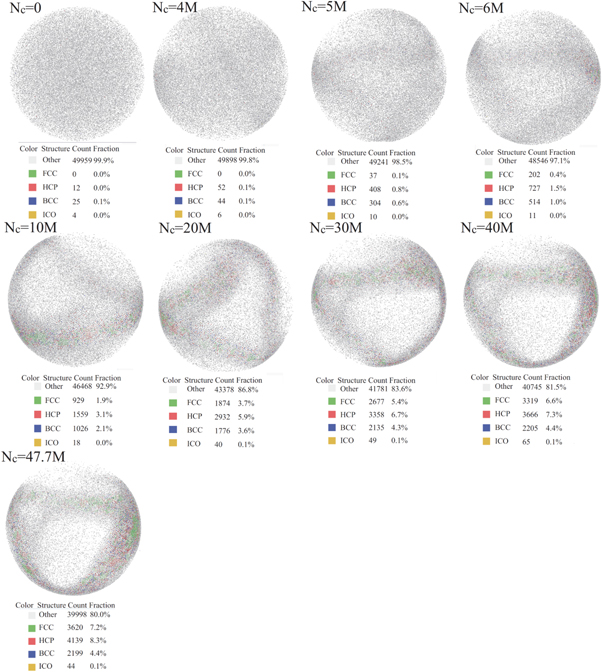
Figure 34. Snapshots of categorized coordination per a granular particle and its fraction obtained using BAA at Nc = 0, 4M, 5M, 6M, 10M, 20M, 30M, 40M and 47.4M, when N = 5 × 10⁴.
Download figure:
Standard image High-resolution imageFigure 35 shows the fractions of the categories of the coordination versus Nc obtained using the BAA (Other: left frame, FCC, HCP, BCC and ICO: right frame). The enlarged figure (log-log plot of the fraction of Other versus Nc) is added to the left frame of figure 35 in order to show that the fraction of Other decreases by the inverse power law function of Nc. As shown in figure 35, the fraction of the category of the coordination is invariant during Nc < 4M and decreases in accordance with  . Then, we can discriminate the topological phase of the granular spheres between Nc < 4M (HCS) and 4M≤Nc (growth of clusters). Reminding that the lsd for d = 0 changes from the log-concave to the log-convex at 3M< Nc < 4M, as shown in figure 29, the BAA also specifies the topological phase-transition of the granular spheres with a similar accuracy to the lsd obtained using d = 0-PD.

Figure 35. Fractions of categories of coordination versus Nc obtained using BAA (Other: left frame, FCC, HCP, BCC and ICO: right frame).
Download figure:
Standard image High-resolution image4.2. Results of VA
Figure 36 shows the snapshots of the categorized coordination per a granular sphere and its fraction at Nc = 0, 2M 4M, 5M, 6M, 10M, 20M, 30M, 40M and 47.4M obtained using the VA. We can confirm that 3.1% of randomly located granular spheres at Nc = 0 can be categorized as HCP or FCC (coordination). Finally, 32.8% of granular spheres obtain the crystal structures, namely, FCC, HCP, BCC, FCC-HCP and ICO at Nc = 47.7M.
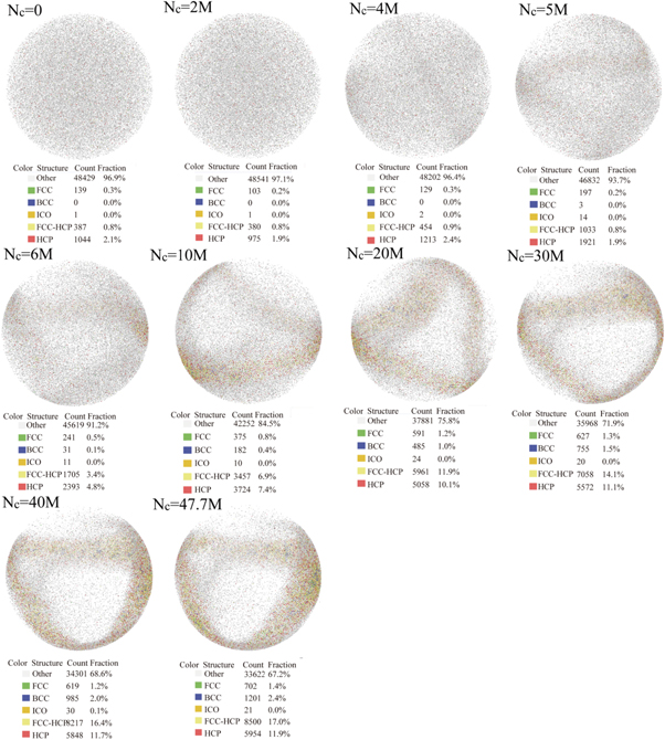
Figure 36. Snapshots of classification of granular gases obtained using VA analysis at  and 47.4M, when N = 5 × 10⁴.
Download figure:
Standard image High-resolution imageFigure 37 shows the fractions of the categories of the coordination versus Nc obtained using the VA (Other: left frame, FCC, BCC, ICO, FCC-HCP and HCP: right frame). The enlarged figure (log-log plot of the fraction of Other versus Nc) is added to the left frame of figure 34 in order to show that the fraction of Other decreases by the inverse power law function of Nc. As shown in figure 34, the fraction of the category Other is almost invariant during Nc < 4M and decreases in accordance with  . Then, the VA-results indicate that the topological phase-transition of the granular spheres occurs between Nc < 4M (HCS) and 4M≤Nc (growth of clusters) similarly to the PD and BAA. The growths of the fractions of the FCC-HCP and HCP are markedly larger than those of the BCC, ICO and FCC. Then, we can conclude that the HCP type coordination is dominant in both cases of the BAA and VA, when the structured coordination are assigned to granular spheres.
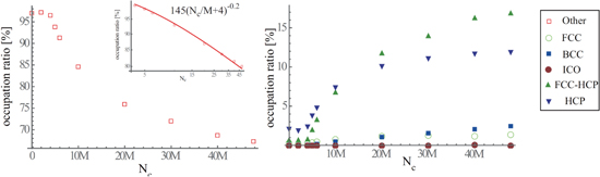
Figure 37. Fractions of categories versus Nc obtained using VA (Other: left frame, FCC, HCP, ICO, FCC-HCP and SC: right frame).
Download figure:
Standard image High-resolution image4.3. Results of PTM
We consider the categorization of the coordination obtained using the PTM. Figures 38–46 show granular particles inside the SP boundary, which are colored in accordance with the assigned category of the coordination (i.e., All:=Other, FCC, HCP, BCC, ICO and SC), at Nc = 0, 4M, 5M, 6M, 10M, 20M, 30M, 40M, and 47.7M together with  versus ℓRMSD (XX:=FCC, HCP, BCC, ICO and SC) in their top-left frames. Additionally, other remained frames except for top-left frame in figures 38–46 show the granular particles inside the SP boundary, which are colored by only two categories Other and XX (XX:=FCC, HCP, BCC, ICO and SC) together with the distribution of the RMSD, namely,
  versus
  , when all the granular particles are categorized by Other and XX (i.e., FCC, HCP, BCC, ICO and SC). Figure 38 shows that 48.7% of N is categorized as Other, whereas 45.3% of N is categorized as the SC and 4.9% of N is categorized as the HCP, at Nc = 0. Then, 50.2% of N is categorized as the structured coordination at Nc = 0, even when the BAA and VA categorize most of N as Other.
  and
and  seem to follow Gaussian distributions at Nc = 0, respectively. The deviations of
  from the Gaussian become marked, as Nc increases. For example,
  has fat tailed distribution at Nc = 10M and has markedly asymmetric form, when 30M≤Nc. In particular, the fat tailed regime of
  at
at  is caused by the plateau distribution of
  at
at  and bimodal distribution of
  at
at  , as shown in figures 44, 45 and 46. Similarly, asymmetry of
  becomes marked, when 10M≤Nc. Other significant result obtained using the PTM is time-evolutions of
  .
.  approaches
  (
( ), as Nc increases. Therefore, most of granular particles, which are categorized as the HCP, deviates from the HCP template with the constant distance 0.27 and such
  decreases exponentially, as
  deviates from 0.27.

Figure 38. Snapshots of fractions of all categories, Other+HCC, Other+HCP, Other+BCC, Other+ICO, and Other+SC and their Root-Mean-Square-Deviation (RMSD) distributions at Nc = 0 obtained using PTM.
Download figure:
Standard image High-resolution image
Figure 39. Snapshots of fractions of all categories, Other+HCC, Other+HCP, Other+BCC, Other+ICO, and Other+SC and their Root-Mean-Square-Deviation (RMSD) distributions at Nc = 4M obtained using PTM.
Download figure:
Standard image High-resolution image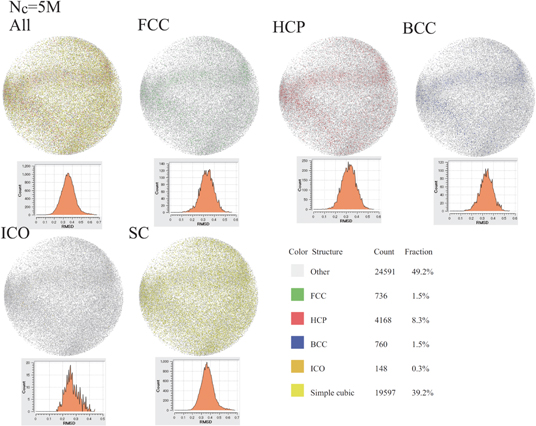
Figure 40. Snapshots of fractions of all categories, Other+HCC, Other+HCP, Other+BCC, Other+ICO, and Other+SC and their Root-Mean-Square-Deviation (RMSD) distributions at  obtained using PTM.
Download figure:
Standard image High-resolution image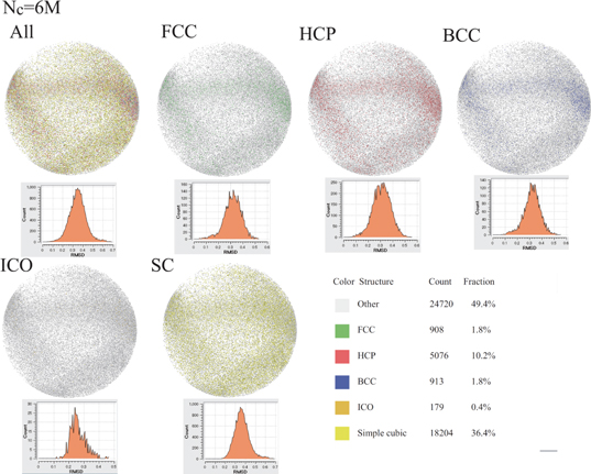
Figure 41. Snapshots of fractions of all categories, Other+HCC, Other+HCP, Other+BCC, Other+ICO, and Other+SC and their Root-Mean-Square-Deviation (RMSD) distributions at Nc = 6M obtained using PTM.
Download figure:
Standard image High-resolution image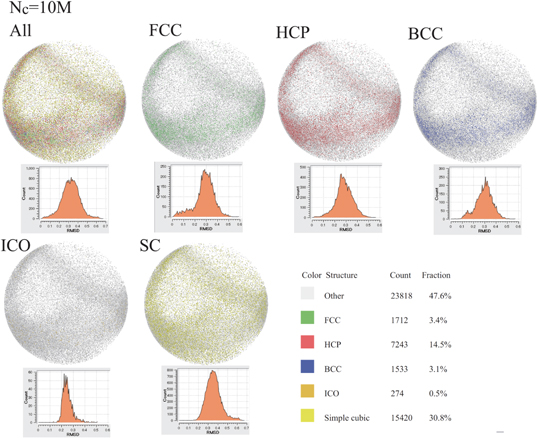
Figure 42. Snapshots of fractions of all categories, Other+HCC, Other+HCP, Other+BCC, Other+ICO, and Other+SC and their Root-Mean-Square-Deviation (RMSD) distributions at  obtained using PTM.
Download figure:
Standard image High-resolution image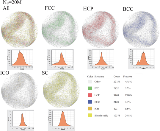
Figure 43. Snapshots of fractions of all categories, Other+HCC, Other+HCP, Other+BCC, Other+ICO, and Other+SC and their Root-Mean-Square-Deviation (RMSD) distributions at Nc = 20M obtained using PTM.
Download figure:
Standard image High-resolution image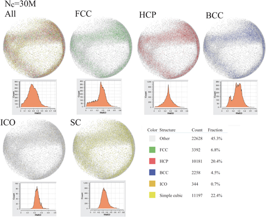
Figure 44. Snapshots of fractions of all categories, Other+HCC, Other+HCP, Other+BCC, Other+ICO, and Other+SC and their Root-Mean-Square-Deviation (RMSD) distributions at Nc = 30M obtained using PTM.
Download figure:
Standard image High-resolution image
Figure 45. Snapshots of fractions of all categories, Other+HCC, Other+HCP, Other+BCC, Other+ICO, and Other+SC and their Root-Mean-Square-Deviation distributions (RMSD) at Nc = 40M obtained using PTM.
Download figure:
Standard image High-resolution image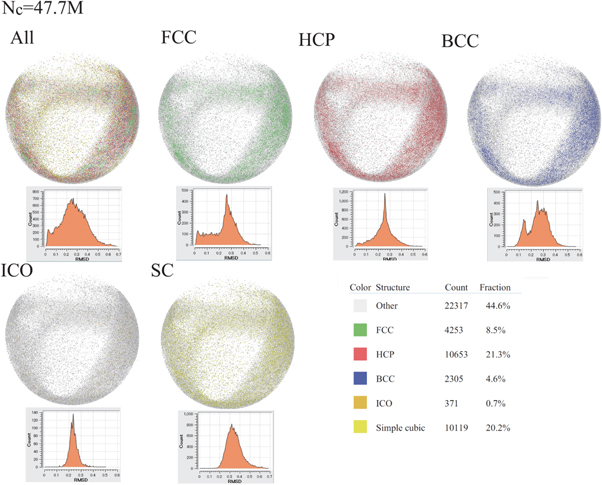
Figure 46. Snapshots of fractions of all categories, Other+HCC, Other+HCP, Other+BCC, Other+ICO, and Other+SC and their Root-Mean-Square-Deviation (RMSD) distributions at Nc = 47.7M obtained using PTM.
Download figure:
Standard image High-resolution imageFinally, the left-top frame of figure 47 shows time-evolution of the fraction of categories XX (:=Other, FCC, HCP, BCC, ICO and SC). The fraction of the HCP increases and becomes comparable with that of the SC, as Nc increases. The temporal change in the fraction of Other is not marked in comparison of that obtained using the BAA and VA. The bottom-left and bottom-right frames show good fits of fractions of categories Other and SC with the inverse-power-law functions, namely,  and
and  , respectively. The deviations from the inverse-power-law functions become marked at Nc ≥ 30M in the case of the SC.
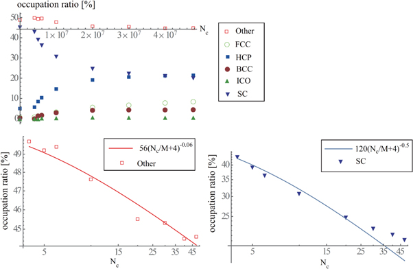
Figure 47. Fractions of categories versus Nc obtained using PTM analysis (top-left frame frame). Log-Log plot of fraction of category Other versus Nc together with its fitting function (line) in bottom-left frame and Log-Log plot of fraction of category SC versus Nc together with its fitting function (line) in bottom-right frame.
Download figure:
Standard image High-resolution image5. Concluding remarks
We investigated the transition from the homogeneous cooling state (HCS) to the pattern formation of the granular gases confined by the elastic wall using the topological analyses, namely, PH, BAA, VA and PTM. The topological phase-transition is successfully identified by the switch of the life-span-distribution (lsd) between the log-concave and log-convex, when the dimension of homology is zero and unity in the cases of the SQ and CI boundaries or zero in the case of the SP boundary. The zeroth and first order Betti numbers obtained using the SQ boundary indicate that three topological phases exist, whereas the zeroth and first order Betti numbers obtained using the CI boundary indicate that only two topological phases exist. The analyses of coordination of granular spheres on the basis of the BAA, VA and PTM indicate that the time-evolution of fractions of categories also become standard to judge the topological phase-transition as well as the switch of the lsd between the log-concave and log-convex. The HCP coordination is dominant, when the condensed granular spheres around the wall are categorized as the structured coordination after the adequate time passes by. Finally, we confirmed that these topological analyses, which have been applied to crystal or glass, are also useful for the consideration of the phase-transition of the granular gases.
Acknowledgments
The authors acknowledge the professor Takahito Kashiwabara (Graduate school of Mathematical Science, University of Tokyo, Japan) for his helpful comments on the specific of homcloud and professor Andrés Santos (Departamento de Fsica, Universidad de Extremadura, Spain) for his helpful comments on the rotation of cluster of granular particles along the wall.
Appendix A.: Simplicial complex
The notion of simplicial complex [33] is a generalization of both of polygons and polyhedrons with triangle faces. It is combinatorially constructed by gluing some basic geometric objects called simplices. For a non-negative integer p, the p-simplex is formally given by a subspace of  formed by (t0 , t1 , ⋯ , tp ) such that
  . In the literature, a subspace of a Euclidean space which is linearly isomorphic to the above p-simplex is also called a p-simplex. For example, the notions of 0-simplices, 1-simplices, 2-simplices and 3-simplices coincide with those of points, line segments, triangles and tetrahedrons respectively. We note that polygons are constructed by gluing some line segments along their boundaries in a proper way. Likewise, polyhedrons with triangle faces are constructed by gluing some triangles along their boundaries in a proper way. Then the notion of simplicial complex is defined by a geometric object which is combinatorially constructed by gluing some simplices.
Appendix B.: Homology
The p-th Betti number is defined via the p-th homology theory. The p-th homology theory is, roughly speaking, the vector space formally generated by p-dimensional holes. We refer the readers to Hatcher's book [20] for exact definitions. The p-th homology theory of a simplicial complex X is usually denoted by  or Hp (X). For example, if we write by X the simplicial complex in figure 3, then the p-th homology theory Hp (X ) is calculated to be a 1-dimensional vector space for p = 0 and 2-dimensional vector space for p = 1 as we give a heuristic discussion in the previous subsection. Moreover, the p-th homology theory Hp (X) is a 0-dimensional vector space for p ≥ 2.
The p-th Betti number is defined by the dimension of the vector space Hp (X). Since the homology theory is based on vector spaces not on numbers as the Betti number, it becomes possible to deal with linear homomorphisms between them. It makes us to obtain more rich information about given simplicial complexes than the Betti number does.
Appendix C.: Persistent homology
The p-th persistent homology is, formally speaking, the persistence module induced by a filtration of a simplicial complex. For the convenience of the readers, we unpack the definition as follows. The p-th persistent homology of a filtration Xt of a simplicial complex X is given by the following data,
- A sequence of vector spaces where Hp denotes the p-th homology theory. See section B.
- A family of linear homomorphisms, for t0 < t1 such that for . It is induced by the inclusion maps .


Note that we deal with finite simplicial complexes so that each vector space Mt is finite-dimensional. A persistence module with finite-dimensional components is called to be pointwise finite-dimensional. By Crawley-Boevey [34], any pointwise finite-dimensional persistence module is a direct sum of interval modules. An interval module is a persistence module  such that for some interval I in the real line,

and
For the p-th persistent homology  of a filtration, we can take a decomposition of interval modules by Crawley-Boevey. Let
  be an interval module component on an interval I as above. If
  are endpoints of the interval I, then we say that the p-th dimensional hole is born at t = a and dead at t = b. By using an interval module decomposition, we obtain the PD.