
Abstract
We solve the D- dimensional Klein–Gordon equation with a newly proposed generalized hyperbolic potential model, under the condition of equal scalar and vector potentials. The relativistic bound state energy equation has been obtained via the functional analysis method. We obtained the relativistic and non-relativistic ro-vibrational energy spectra for different diatomic molecules. The numerical results for these diatomic molecules tend to portray inter-dimensional degeneracy symmetry. Variations of the energy eigenvalues obtained with the potential parameters have been demonstrated graphically. Our studies will find relevant applications in the areas of chemical physics and high-energy physics.
Export citation and abstract BibTeX RIS

Original content from this work may be used under the terms of the Creative Commons Attribution 3.0 licence. Any further distribution of this work must maintain attribution to the author(s) and the title of the work, journal citation and DOI.
Corrections were made to this article on 28 10 2020. The author list was rearranged.
Introduction
Researchers over the years have continually sought for solutions of wave equations with potential energies both in the non-relativistic and relativistic quantum mechanical systems [1, 2]. These solutions will provide all the necessary information needed to explain the behavior of any physical system. In addition, the solutions of these wave equations are highly applicable in chemical physics and high-energy physics at higher spatial dimensions [3]. Klein–Gordon (KG) equation is a basic relativistic wave equation that is well known to describe the motion of spin zero particles [4]. Different investigations have been carried out to obtain the exact and approximate solutions of the KG equation with different potentials, via various methods including the asymptotic iteration method (AIM) [5], Nikiforov-Uvarov (NU) method [6], supersymmetric quantum mechanics (SUSYQM) [7], algebraic approach [8], exact and proper quantization rules [9], modified factorization method [10, 11] and others [12–16].Many authors have studied the solutions of the D-dimensional Klein–Gordon equation with diatomic molecular potential energy models [17–25]. Analytical solutions of the KG equation and Dirac equation have been obtained for the conventional form of the Rosen-Morse (RM) potential energy model [26, 27]. Chen and his collaborators [28] studied the relationship between the D-dimensional relativistic ro-vibrational energies with applications to the Lithium diatomic molecule. In addition, RM type scalar and vector potential energy model was employed to obtain the s-wave bound state energy spectra [29]. Villalba et al [30] considered the bound state solution of a one-dimensional Cusp potential model, confined in the KG equation. The bound state solution of the KG equation with mixed vector and scalar PT potential energy with a nonzero angular momentum parameter was investigated by Xu et al [31]. Badalov et al [32] used NU to study any l-state of the KG equation, with the help of a Pekeris-like approximation scheme. In similar development, Ikot et al [33] solved the KG equation with the Hylleraas potential model and obtained its exact solution. Also, Hassanabadi and his collaborators [20] studied a combined Eckart potential and modified Hylleraas potential energy in higher dimensional KG equations using supersymmetric quantum mechanics method. Jia et al [22] investigated the bound state solution of the KG equation with an improved version of the Manning-Rosen potential model. Ortakaya [34] solved the D-dimensional KG equation and obtained the bound state energy spectrum for three different diatomic molecules using pseudoharmonic oscillator potential model. Chen et al [28] employed the improved MR potential energy in D-spatial dimensions to obtain the relativistic bound state energy equation. Also, Ikot et al [35] analyzed the improved MR potential energy for arbitrary angular momentum parameter using an approximate method in D-dimensions. Xie et al [36] studied the bound state solutions of the KG equation with the Morse potential energy in D-spatial dimensions. Ikot and his co-authors [37] employed NU method to investigate the D-dimensional KG equation with an exponential type molecule potential model. Hyperbolic potential models have been used as the empirical mathematical models in describing various inter-atomic interactions for diatomic and polyatomic molecules [38]. Deformed hyperbolic functions have also been studied and its non-relativistic energy spectra obtained via different methods [39–44].Most recently, Durmus [45] studied the Dirac equation with equal scalar and vector hyperbolic potential function using the AIM, with the help of Greene and Aldrich approximation scheme. The author also investigated the relativistic vibrational energy spectra for various electronic states of some alkali metal diatomic molecules.Motivated by the work of Durmus [45], we propose a generalized hyperbolic potential (GHP) of the form

where  are potential parameters, and
  is the range of the potential.
Using the functional analysis method, we investigate the approximate bound state solution of the KG equation with GHP in higher spatial dimensions. We also explore the properties of the D-dimensional relativistic and non-relativistic ro-vibrational energy spectra for the GHP analytically and numerically for some selected diatomic molecules.
Bound state solutions
The Klein–Gordon equation with a scalar potential  and a vector potential
  in D-dimensions reads [46]

where  represents the spatial dimensionality and
  represents the Laplace operator in D-dimensions,
  is the reduced Planck constant,
  and
and  are the speed of light and relativistic energy of the system, respectively. Also, the wave function can be given as
  where
where  is the generalized spherical harmonic function. Employing the eigenvalues of the generalized angular momentum operator
  where
where

we write the radial part of the D-dimensional Klein–Gordon equation (2) as

where 
 represents the relativistic ro-vibrational energy eigenvalues in D-dimensions,
  represents the vibrational and rotational quantum numbers, respectively. For equal scalar and vector potentials,
  equation (4) becomes

Rescaling the scalar potential  and vector potential
  under the non-relativistic limit, we adopt the Alhaidari et al [47] scheme to write equation (4) as

With the equal scalar and vector potential being taken as the generalized hyperbolic potential, we obtain the following second-order Schrodinger-like equation as,

Due to the presence of the centrifugal term in equation (7), we employ the Greene-Aldrich approximation scheme [48]

As noted in [45], the above approximation is seen to be valid only for short range potential with small potential range,  This approximation tends to break down for large
Substituting equation (8) and introducing coordinate transformation of the form  we get

where


Also, we propose the wave function as

where


We find that equation (9) turns into a Gauss hypergeometric-type equation of the form

where

The solution of equation (16) can be expressed in terms of the hypergeometric function given below

where


To obtain the energy relation, we equate either equations (19) or (20) to a negative integer (say  ). Hence, we choose

Substituting equations (10)–(12), (14), (15) and (17) into (22), we obtain the D-dimensional relativistic ro-vibrational energy spectra for the GHP in the form
To obtain the nonrelativistic ro-vibrational energy spectra for the GHP, we employ the following mapping:  With these mapping we obtain

The normalization of the wave function can be determined as shown in appendix appendix.
Results and discussion
We consider different diatomic molecules ( ) with spectroscopic parameters as shown in table 1. These parameters were adopted from [49] and applied to equation (24) to compute the numerical values of the non-relativistic ro-vibrational energies for arbitrary quantum numbers in different dimensions, as shown in tables 2–5. We observe from the tables presented that the non-relativistic ro-vibrational energies for the selected diatomic molecules decrease as the quantum numbers (
 ) increase. Also, for any quantum state, there is a decrease in ro-vibrational energies as the dimension increases. This trend is consistent with the relation of energy eigenvalues and quantum numbers, as observed in [49] for the selected diatomic molecules. In addition, we observe that there exist an inter-dimensional degeneracy symmetry for the selected diatomic molecules (
 ). This implies that the nonrelativisticro-vibrational energy spectra for the GHP is invariant under a transformation of an increase in the D-dimension by two (
 ) and a decrease in the rotational quantum number by one (
 ).
).
Table 1. Spectroscopic Parameters for the selected diatomic molecules.
| Molecule |

|

|
|---|---|---|

|

|

|

|

|

|

|

|

|

|

|

|
Table 2. Energy spectra  of
of  for arbitrary
  quantum numbers at different dimensions with

|

|

|

|

|

|
|---|---|---|---|---|---|

|

| 3.992 561 016 | 3.992 363 344 | 3.992 028 341 | 3.991 547 708 |

|

| 3.933 049 146 | 3.932 458 722 | 3.931 469 539 | 3.930 073 901 |

| 3.931 469 539 | 3.930 073 901 | 3.928 261 090 | 3.926 017 406 | |

|

| 3.814 025 405 | 3.813 042 230 | 3.811 398 865 | 3.809 088 223 |

| 3.811 398 865 | 3.809 088 223 | 3.806 100 428 | 3.802 422 859 | |

| 3.806 100 428 | 3.802 422 859 | 3.798 040 210 | 3.792 934 558 | |

|

| 3.635 489 793 | 3.634 113 867 | 3.631 816 322 | 3.628 590 675 |

| 3.631 816 322 | 3.628 590 675 | 3.624 427 896 | 3.619 316 441 | |

| 3.624 427 896 | 3.619 316 441 | 3.613 242 314 | 3.606 189 122 | |

| 3.613 242 314 | 3.606 189 122 | 3.598 138 150 | 3.589 068 449 | |

|

| 3.397 442 311 | 3.395 673 633 | 3.392 721 908 | 3.388 581 256 |

| 3.392 721 908 | 3.388 581 256 | 3.383 243 494 | 3.376 698 152 | |

| 3.383 243 494 | 3.376 698 152 | 3.368 932 548 | 3.359 931 814 | |

| 3.368 932 548 | 3.359 931 814 | 3.349 678 989 | 3.338 155 080 | |

| 3.349 678 989 | 3.338 155 080 | 3.325 339 141 | 3.311 208 372 |
Table 3. Energy spectra  of
of  for arbitrary
  quantum numbers at different dimensions with

|

|

|

|

|

|
|---|---|---|---|---|---|

|

| 3.998 936 343 | 3.998 925 695 | 3.998 907 833 | 3.998 882 582 |

|

| 3.990 427 085 | 3.990 395 196 | 3.990 341 934 | 3.990 267 130 |

| 3.990 341 934 | 3.990 267 130 | 3.990 170 545 | 3.990 051 877 | |

|

| 3.973 408 571 | 3.973 355 439 | 3.973 266 777 | 3.973 142 419 |

| 3.973 266 777 | 3.973 142 419 | 3.972 982 135 | 3.972 785 627 | |

| 3.972 982 135 | 3.972 785 627 | 3.972 552 536 | 3.972 282 432 | |

|

| 3.947 880 799 | 3.947 806 425 | 3.947 682 363 | 3.947 508 452 |

| 3.947 682 363 | 3.947 508 452 | 3.947 284 466 | 3.947 010 120 | |

| 3.947 284 466 | 3.947 010 120 | 3.946 685 062 | 3.946 308 875 | |

| 3.946 685 062 | 3.946 308 875 | 3.945 881 084 | 3.945 401 147 | |

|

| 3.913 843 769 | 3.913 748 153 | 3.913 588 691 | 3.913 365 226 |

| 3.913 588 691 | 3.913 365 226 | 3.913 077 541 | 3.912 725 356 | |

| 3.913 077 541 | 3.912 725 356 | 3.912 308 331 | 3.911 826 061 | |

| 3.912 308 331 | 3.911 826 061 | 3.911 278 086 | 3.910 663 877 | |

| 3.911 278 086 | 3.910 663 877 | 3.909 982 851 | 3.909 234 363 |
Table 4. Energy spectra  of
of  for arbitrary
  quantum numbers at different dimensions with

|

|

|

|

|

|
|---|---|---|---|---|---|

|

| 3.998 389 228 | 3.998 369 374 | 3.998 336 020 | 3.998 288 766 |

|

| 3.985 503 049 | 3.985 443 611 | 3.985 344 290 | 3.985 204 702 |

| 3.985 344 290 | 3.985 204 702 | 3.985 024 308 | 3.984 802 416 | |

|

| 3.959 730 692 | 3.959 631 668 | 3.959 466 381 | 3.959 234 459 |

| 3.959 466 381 | 3.959 234 459 | 3.958 935 382 | 3.958 568 482 | |

| 3.958 935 382 | 3.958 568 482 | 3.958 132 944 | 3.957 627 808 | |

|

| 3.921 072 156 | 3.920 933 547 | 3.920 702 294 | 3.920 378 038 |

| 3.920 702 294 | 3.920 378 038 | 3.919 960 277 | 3.919 448 368 | |

| 3.919 960 277 | 3.919 448 368 | 3.918 841 526 | 3.918 138 822 | |

| 3.918 841 526 | 3.918 138 822 | 3.917 339 193 | 3.916 441 430 | |

|

| 3.869 527 441 | 3.869 349 248 | 3.869 052 028 | 3.868 635 438 |

| 3.869 052 028 | 3.868 635 438 | 3.868 098 994 | 3.867 442 076 | |

| 3.868 098 994 | 3.867 442 076 | 3.866 663 929 | 3.865 763 658 | |

| 3.866 663 929 | 3.865 763 658 | 3.864 740 239 | 3.863 592 508 | |

| 3.864 740 239 | 3.863 592 508 | 3.862 319 173 | 3.860 918 810 |
Table 5. Energy spectra  of
of  for arbitrary
  quantum numbers at different dimensions with

|

|

|

|

|

|
|---|---|---|---|---|---|

|

| 3.999 885 513 | 3.999 885 138 | 3.999 884 511 | 3.999 883 630 |

|

| 3.998 969 616 | 3.998 968 491 | 3.998 966 614 | 3.998 963 983 |

| 3.998 966 614 | 3.998 963 983 | 3.998 960 595 | 3.998 956 447 | |

|

| 3.997 137 823 | 3.997 135 948 | 3.997 132 820 | 3.997 128 439 |

| 3.997 132 820 | 3.997 128 439 | 3.997 122 801 | 3.997 115 903 | |

| 3.997 122 801 | 3.997 115 903 | 3.997 107 740 | 3.997 098 308 | |

|

| 3.994 390 134 | 3.994 387 508 | 3.994 383 130 | 3.994 376 999 |

| 3.994 383 130 | 3.994 376 999 | 3.994 369 110 | 3.994 359 462 | |

| 3.994 369 110 | 3.994 359 462 | 3.994 348 049 | 3.994 334 866 | |

| 3.994 348 049 | 3.994 334 866 | 3.994 319 908 | 3.994 303 167 | |

|

| 3.990 726 547 | 3.990 723 171 | 3.990 717 544 | 3.990 709 662 |

| 3.990 717 544 | 3.990 709 662 | 3.990 699 523 | 3.990 687 124 | |

| 3.990 699 523 | 3.990 687 124 | 3.990 672 461 | 3.990 655 528 | |

| 3.990 672 461 | 3.990 655 528 | 3.990 636 319 | 3.990 614 829 | |

| 3.990 636 319 | 3.990 614 829 | 3.990 591 048 | 3.990 564 970 |
Furthermore, we represent equation (24) in 3-dimensions as follows (where  in 3-dimensions)

For  the generalized hyperbolic potential of equation (1) reduces to

and its corresponding nonrelativisticro-vibrational energy spectra is obtained as

The result in equation (27) is very consistent with [45, 50]. This results' accuracy have been tested by calculating the ro-vibrational energy spectra of the equation (27) numerically for different quantum states and various potential range, We have compared our result with other results obtained using different methods such as AIM [45] and algebraic method [50], as shown in table 6.
Table 6. Comparison of energy spectra  for special case of generalized hyperbolic potential in D-dimensions for arbitrary quantum states with
| States |

| Present work | AIM [45] | Algebraic method [50] |
|---|---|---|---|---|

|

| −3.575 101 020 | −3.575 101 016 | −3.575 101 02 |

| −3.166 384 390 | −3.166 384 378 | −3.166 384 38 | |

| −2.773 782 467 | −2.773 782 451 | −2.773 782 46 | |

| −2.397 227 654 | −2.397 227 633 | −2.397 227 65 | |

| −2.036 652 400 | −2.036 652 376 | −2.036 652 40 | |

|

| −3.246 181 840 | −3.246 181 829 | −3.246 181 83 |

| −2.543 491 901 | −2.543 491 882 | −2.543 491 90 | |

| −1.891 808 441 | −1.891 808 414 | −1.891 808 44 | |

| −1.291 009 778 | −1.291 009 744 | −1.291 009 77 | |

| −0.740 974 322 | −0.740 974 285 | −0.740 974 32 | |

|

| −2.927 262 658 | −2.927 262 642 | −2.927 262 65 |

| −1.960 599 413 | −1.960 599 387 | −1.960 599 41 | |

| −1.099 834 416 | −1.099 834 381 | −1.099 834 41 | |

| −0.344 791 902 | −0.344 791 861 | −0.344 791 90 | |

| 0.304 703 7560 | 0.304 703 798 | 0.304 703 753 | |

|

| −2.771 553 066 | −2.771 553 048 | −2.771 553 06 |

| −1.684 153 169 | −1.684 153 139 | −1.684 153 17 | |

| −0.737 597 4030 | −0.737 597 365 | −0.737 597 40 | |

| 0.068 317 0360 | 0.068 317 079 | 0.068 317 035 | |

| 0.733 792 7940 | 0.733 792 837 | 0.733 792 792 |
We also set  to have hyperbolic Rosen-Morse potential from the GHP in the form

The non-relativistic ro-vibrational energy spectra of the hyperbolic Rosen-Morse potential is obtained to be

We also plot the graphs of the non-relativistic ro-vibrational energies with respect to the potential range, dimensions, rotational and vibrational quantum numbers, potential parameters, as shown in figures 1–8, respectively. From figures 1–4 respectively, it is seen that there is a monotonic decrease in the non-relativistic energies as  increases for the selected diatomic molecules. Figures 5 and 6 show the increase in
  as the potential parameters
  increases, respectively. In figures 7 and 8, the non-relativistic ro-vibrational energies increases to a peak value and later decreased as the potential parameters
  increases, respectively. In addition, we considered the variation of
  with spatial dimension
  for various quantum states of
  molecule as shown in figure 9. As the spatial dimension increases, the non-relativistic ro-vibrational energy
  decreases slowly and later decreases in a monotonic manner. Figure 10 shows a sharp decrease in
  as the vibrational quantum number increases for different spatial dimensions of
  molecule.

Figure 1. Nonrelativistic ro-vibrational energy versus  for various diatomic. Molecules and
Download figure:
Standard image High-resolution image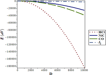
Figure 2. Nonrelativistic ro-vibrational energy versus  for various diatomic. Molecules and
Download figure:
Standard image High-resolution image
Figure 3. Nonrelativistic ro-vibrational energy versus  for various diatomic. Molecules and
Download figure:
Standard image High-resolution image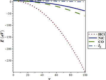
Figure 4. Nonrelativistic ro-vibrational energy versus  for various diatomic. Molecules and
Download figure:
Standard image High-resolution image
Figure 5. Nonrelativistic ro-vibrational energy versus  for various diatomic. Molecules and
Download figure:
Standard image High-resolution image
Figure 6. Nonrelativistic ro-vibrational energy versus  for various diatomic. Molecules and
Download figure:
Standard image High-resolution image
Figure 7. Nonrelativistic ro-vibrational energy versus  for various diatomic. Molecules and
Download figure:
Standard image High-resolution image
Figure 8. Nonrelativistic ro-vibrational energy versus  for various diatomic. Molecules and
Download figure:
Standard image High-resolution image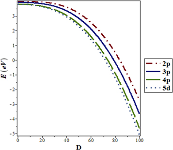
Figure 9. Nonrelativistic ro-vibrational energy for  molecule versus
  for. various quantum states.
Download figure:
Standard image High-resolution image
Figure 10. Nonrelativistic ro-vibrational energy for  molecule versus
  for. various
  and
and 
Download figure:
Standard image High-resolution imageConclusion
In our study, we solve the D-dimensional Klein–Gordon (KE) equation with our newly proposed generalized hyperbolic potential (GHP) model using the functional analysis method. By employing the Greene-Aldrich-like approximation scheme, we obtain an expression for the D-dimensional relativistic ro-vibrational energy spectra for the GHP. Also, this expression was reduced to the non-relativistic case by employing the necessary mapping scheme. Numerical results for the D-dimensional non-relativistic ro-vibrational energy spectra were obtained for different diatomic molecules ( ), for arbitrary quantum numbers. Special cases were obtained where our results agree with the results obtained in the literature. Our results for different diatomic molecules show inter-dimensional degeneracy symmetry as the dimensions increase and the rotational quantum number decreases. Different plots of non-relativistic ro-vibrational energy spectra versus the GHP parameters were also analyzed and discussed. These plots show a monotonic decrease in the energy eigenvalues as the potential parameters increase for the diatomic molecules considered. A specific consideration was given to
  molecule, as the variation of its non-relativistic ro-vibrational energy eigenvalues with both D-spatial dimension and vibrational quantum numbers, respectively, were discussed.
Acknowledgments
The authors thank the kind reviewers for the positive comments and suggestions that lead to an improvement of our manuscript


