
Abstract
A power law model for cavitation erosion is proposed herein that represents volume loss as the creation and subsequent enlargement of hemispherical pits in the surface of the solid. The cumulative volume loss (CVL) of a material is expressed as an Arrhenius term, containing the energy of pit growth, Epg, multiplied by a power law function with the pit radius growth rate, k, as a prefactor and a time exponent, n. The model is verified through fitting of experimental cavitation erosion data for commercially-available aluminum, copper, and zinc substrates, as well as fitting selected data from the International Cavitation Erosion Test and through comparison with other cumulative volume loss models.
Export citation and abstract BibTeX RIS

Original content from this work may be used under the terms of the Creative Commons Attribution 3.0 licence. Any further distribution of this work must maintain attribution to the author(s) and the title of the work, journal citation and DOI.
1. Introduction
Cavitation erosion—the erosion of a hard surface due to propagation of sound waves in an adjacent fluid—has been viewed as an understandably detrimental phenomenon in most of the published literature. It shortens the lifetime of components and can lead to part failure in a number of important technological settings, including hydroelectric dams [1] and fluids processing [2]. In fact, anywhere that hard surfaces come in contact with flowing fluids there is a possibility of cavitation, which can lead to cavitation erosion of the surface. This phenomenon need not be avoided in all circumstances. An emergent field of cavitation erosion study, Reactive Cavitation Erosion (RCE) [3], harnesses cavitation erosion resulting from the purposeful introduction of sound waves into a fluid to produce nanostructured materials from the solid surface, termed acoustic cavitation erosion.
Modeling of cavitation erosion before the emergence of RCE often utilized metrics such as erosion rate [4–7], incubation period [8], mean depth of erosion/penetration (MDE/MDP) [9], mean depth of erosion/penetration rate (MDER/MDPR) [10, 11], and mass/volume loss [12, 13]. The erosion rate is calculated through numerical differentiation of mass loss data and due to the difficulty in continuous monitoring of the mass loss is inherently inaccurate. The incubation period is the amount of time a substrate must be exposed to cavitation erosion for measurable mass loss to occur. This metric does not provide information on the erosion behavior of the material after this characteristic time. The MDE or MDP, determined by dividing the observed mass loss data by the density of the eroded material and the total exposed surface area, assumes that the surface damage induced by cavitation erosion is spatially uniform over the total exposed surface. But this assumption is flawed. There is evidence in the literature showing that the damage is not spatially uniform [14]. This disregard for the spatial distribution of damage leads to a calculated MDE or MDP smaller than the true MDE or MDP. Additionally, MDE/MDP does not give a true representation of surface damage since there are regions where the actual depth of erosion is much higher or much lower than the MDE. Cumulative volume loss (CVL) on the other hand, does not require any assumptions about the spatial distribution of damage. As long as the sample dimensions are the same—as they are in this study—CVL values can be compared. The MDER or MDPR suffers from the same pitfalls as the erosion rate and the MDE or MDP. As opposed to the preceding metrics, mass or volume loss can be directly measured and does not depend on assumptions that may be invalid. For Reactive Cavitation Erosion modeling, the best metric to use is the mass or volume loss since the goal of RCE is to maximize the generation of material from the surface. In order to facilitate material selection for RCE and to better understand the relationship between material properties and process optimization, a model is needed that not only accurately describes the observed mass or volume loss, but also accurately predicts these metrics from previously untested materials.
A power law model for cavitation erosion is proposed herein that represents volume loss - mass loss divided by the density of the eroded material—as the creation and subsequent enlargement of hemispherical pits in the surface of the solid. Justification for this simple geometric model is given. The model is then applied to experimental data from the acoustic cavitation of commercially-available aluminum, copper, and zinc substrates, as well as fitting selected data from the International Cavitation Erosion Test [15].
2. Theory
The cumulative volume loss associated with acoustic cavitation erosion can be modeled as the creation and subsequent enlargement of hemispherical pits. The hemispherical pits are characterized by their radii, r, a schematic of which is shown in figure 1.

Figure 1. Geometric definitions for hemispherical pit model.
Download figure:
Standard image High-resolution imageThe Hemispherical Pit Model begins with an expression for the cumulative volume loss, CVL(t), expressed in terms of the number of pits, N, with volume, V, each potentially a function of time:

For the purposes of this study, we limited the mathematical representation of N(t) to the growth region only; that is, the incubation period for initiation of pits is assumed to be short relative to the growth period such that the number of pits that actually grow, N*, is not a function of time, but rather is an activated process. In this way, N(t) becomes the product of the fixed number of pits that are available to grow at the end of the incubation period, N, times an Arrhenius-type expression that describes the activation energy barrier for pit growth of the eroded material, G:

where G is the fraction of available pits that actually undergo growth due to cavitation erosion

The CVL(t) thus becomes through simple substitution of (2) into (1)

The volume of the pit per unit area of eroded surface can be expressed as

Substitution of equations (5) and (3) into equation (4), followed by integration results in

where

In these equations, CVL(t) is the cumulative volume loss as a function of time, V(t) is the volume of the pit (cm3) at time t (min), N(t) is the number of pits which is assumed to be fixed at N in the growth phase where the subset of N* actually undergo growth, G is the fraction of pits that are growing, k0 is a rate constant for pit growth (cm · min−n) that is proportional to the intensity of cavitation, n is the time exponent (dimensionless), and Epg is the activation energy for pit growth (J · mol−1). This model is thus limited to the case of pit growth, which corresponds to the region of increasing erosion rate described by previous investigators [16]. The model assumes that all pits are formed during the incubation periodic, that pits only exhibit growth with mass loss in the accumulation or transition period immediately following the incubation period, and that pit overlap does not occur on the time scale of interest. During this period, it is also assumed that there are no processes that would lead to the reintegration of eroded material back into the pits by means of entrapment in surface features, meaning that k must have a positive value. This assumption is justified in that—by the very nature of acoustic cavitation—the fluid environment around the test specimen is generally turbulent and any particulate that re-deposits in a pit would likely be removed rapidly.
A routine was created in Matlab R2018a to minimize the sum of squared errors between the integrated form of the cumulative volume loss, equation (6), and the average values of the measured cumulative volume loss for each metal, with the program calculating Epg, k, n, and the goodness of fit, GoF (R2). The routine utilized the built-in Matlab program Multistart, with 200 starting points, coupled with the built-in function fmincon using the sqp algorithm. The Multistart options MaxFunEvals and MaxIter were set to 100,000 and the options TolX, Tolfun, and TolCon were set to 10−9. The fit parameters were constrained to ensure only physically plausible values were obtained as well as to increase the GoF values obtained. The lower and upper bounds for the fit parameters were: −7 × 10⁵ J · mol−1 ≤ Epg ≤ −1 × 10⁵ J · mol−1; 10−7 cm · min−n ≤ k ≤ 10−4 cm · min−n; and 0.1 ≤ n ≤ 1. The initial values for all three parameters were set to 0. Additional statistical parameters χ2 and adjusted R2 were calculated from the hemispherical pit model fit of the data.
Two models were chosen for comparison with the Hemispherical Pit Model: a logistic model proposed by Hattori et al [9] and a Weibull function model proposed by Szkodo [17]. These models were chosen due to the presence of singular analytical expressions that did not rely upon numerical solutions of differential equations, which also allowed for them to be input into the same model fitting framework created for the HPM fittings.
The logistic model developed by Hattori et al is of the form

where V is the cumulative volume loss (cm3), α is the multiplication factor in pit number per unit time, β is the annihilation factor in pit number per unit time, c = (α/β)U0, and U0 is the initial volume loss rate (cm3 · min−1). The ratio α/β represents the maximum erosion rate. The annihilation of pits is assumed to be the combination of pits. When two or more pits increase in size enough so that their boundaries intersect the number of pits effectively decreases; only one pit remains whereas the rest are 'annihilated.' Hattori et al performed cavitation erosion experiments using alumina and copper substrates and fitted the data with the model.
Szkodo modeled the volume loss of material, V(t), at time t as

where the bracketed term is a Weibull function, V is the initial volume of the sample, H is the height of the sample, h is the depth of strain hardening, I is the relative intensity of cavitation, A is the surface area of the sample, Kc is the relative stress intensity factor under cavitation loading, and Wpl is the relative work of plastic deformation. What, exactly, these values are relative to is not explained. Additionally, this model was not fit to experimental data, so no examples of potential parameter values were presented.
3. Experimental methods
Experiments were performed using a modified version of the Standard Test Method for Cavitation Erosion Using Vibratory Apparatuses (ASTM-G32) for stationary specimens. Two sets of experiments were performed: one at a lower temperature of ∼43 °C and one at a higher temperature of ∼86 °C. Three experiments were performed at each temperature with each specimen type. Experimental specimens consisted of 12.7 mm (nominal) discs of Al 6061 (ρ = 2.68 g · cm−3), Cu 110 equivalent to UNS C11000 (ρ = 8.89 g · cm−3), and a titanium-zinc alloy conforming to DIN EN 988 (ρ = 7.10 g · cm−3) with thicknesses of 1.54 ± 0.05 mm, 1.58 ± 0.07 mm, and 1.07 ± 0.06 mm, respectively. Each specimen was wiped with isopropyl alcohol wipes to remove surface contaminants then weighed with an accuracy of 0.1 mg on a microbalance. Each disc was then push-fit into a custom-built Delrin® holder; a steel rod backstop was used with the Al 6061 specimens due to specimen size differences to prevent the discs from being pushed further into the holder during the experiment. The holder was placed in a 50-ml Pyrex glass beaker. The beaker and contents were placed into an aluminum insert situated inside a nylon container to ensure the beaker remained centered. The nylon container and contents were then placed inside a sound abating enclosure (Sonics). For the lower temperature experiments ice and water were added to the nylon container around the beaker to provide sufficient heat transfer. For the higher temperature experiments no heat transfer fluid of any kind was added to the nylon container. A solid Ti-6Al-4V sonotrode with a tip diameter of 13 mm, attached to an ultrasound source operating at a frequency of 20 kHz (Sonics VCX 750) was mounted in a customized holder such that the sonotrode surface was directly in line with and parallel to the disc surface at a separation, δ, of 0.5 mm (figure 2). A K-type thermocouple was positioned approximately halfway between the beaker wall and the sonotrode. Purified water (17.5 ml, Millipore) was added to the beaker to ensure the depth of the specimen surface conformed to ASTM G-32. The specimen was then sonicated at a sonotrode peak-to-peak amplitude of 57 μm for 30 min. For the first five minutes the temperature was recorded every 20 s followed by once every five minutes until the 30 min point. After 30 min, the particle-laden water discarded. The specimen was removed from the holder, rinsed with purified water and then dried under a flowing nitrogen stream prior to weighing. This procedure was repeated until the total sonication time, tsonic, reached two hours. A total of three experiments were performed with each metal, with the reported cumulative volume loss representing the average of the three specimens. The standard deviation of the average cumulative volume loss was also calculated.

Figure 2. Schematic diagram of cavitation erosion apparatus.
Download figure:
Standard image High-resolution image4. Results and discussion
4.1. HPM fitting to experimental results
Plots of the average cumulative volume loss for the Al 6061, Cu 110, and Zn samples at 43 and 86 °C are shown in figure 3. The error bars represent the standard deviation of the cumulative volume loss for the three samples corresponding to each point. The data for all three metals are fitted by the Hemispherical Pit Model (equation (6)). In figure 3, none of the cumulative volume loss plots exhibit evidence of an incubation period, indicating that if such a region exists it is short relative to experimental measurements. There is a discernable difference in the cumulative mass loss values from the 43 °C experiments of Al 6061 and Cu 110 compared to Zn. On the basis of yield strength and hardness of these metals (table 1), Zn might be predicted to exhibit greater cumulative volume loss as it is a softer metal. Variations in other material properties such as the elastic modulus and ultimate strength (table 1) do not provide adequate explanations for the observed cavitation erosion behavior. Crystal structures of the metals, however, may be the determining factor. Al 6061 and Cu 110 are face-centered cubic (FCC) metals while Zn has a hexagonal close packed (HCP) structure. Previous researchers have demonstrated that material removal of FCC metals under cavitation erosion proceeds through ductile rupture or void growth and coalescence mechanisms whereas material removal of HCP metals is due to brittle fracture [18]. The decrease in the difference in cumulative mass loss values for all three metals in the 86 °C experiments is attributed to the decreased cavitation intensity. An increase in temperature is associated with a decrease in fluid viscosity and surface tension along with an increase in vapor pressure. These changes lead to a decrease in bubble stability meaning that the cavitation bubbles that do form will collapse at smaller diameters. Since the diameter of a cavitation bubble at the start of collapse is directly proportional to cavitation intensity, smaller bubbles mean decreased intensity. The decrease in cumulative mass loss at 86 °C compared to 43 °C is in agreement with the published literature [19–21].

Figure 3. Cumulative volume loss data. Lines are HPM fits.
Download figure:
Standard image High-resolution imageTable 1. Material properties of experimental metals.
| Metal | Ultimate tensile strength, σUTS (MPa) | Yield strength, σy (MPa) | Elastic modulus, E (GPa) | Hardness (vickers) |
|---|---|---|---|---|
| Al 6061a | 310 | 276 | 68.9 | 107 |
| Cu 110 | 302b | 292b | 115–130c | 97b |
| Znd | 150–190 | 140 | 80 | 40 |
aValues taken from matweb report on Al 6061-T6 [22]. bValues supplied by the manufacturer. cRange taken from matweb report on Cu 110 [23]. dValues supplied by Rheinzink.
The Hemispherical Pit Model parameter values of the curve fits in figure 3 are shown in table 2. The bounds used for the fittings were: −5 × 10⁴ kJ · mol−1 ≤ Epg ≤ −1 × 10⁴ kJ · mol−1; 1 × 10⁻⁵ cm · min−n ≤ k ≤ 1 × 10⁻² cm · min−n; and 0.01 ≤ n ≤ 0.5. There exists no consistent trend between an increase in temperature and the resultant change in Epg, k, or n for the metals studied: for Al 6061 an increase in temperature leads to an increase in Epg and decreases in both k and n; for Cu the opposite trend is seen; and for Zn there is very little change in Epg, a decrease in k, and an increase in n. We therefore conclude that while the three parameters could be temperature dependent, there is insufficient information from the two temperatures to determine the exact relationship. The energies associated with activated processes are often assumed and shown experimentally to be independent of temperature [24] such that linearization of equation (6) and subsequent plotting of ln (CVL) versus 1/T provides Epg from the slope. Further temperature studies to validate this approach were not possible with the current experimental setup, but are definitely warranted in future studies. The values for the experimentally-determined activation energies are far below those of their respective metallic bond energies and energies for other active processes such as self-diffusion, and more comparable to activation energies for such facile processes as propagation in polymerization reactions [24].
Table 2. Hemispherical pit model parameters.
| Epg (kJ · mol−1) | k (cm · min−n) | n | |
|---|---|---|---|
| Al 43 °C | −22.1 | 9.12 × 10⁻⁴ | 0.21 |
| Al 86 °C | −29.0 | 5.47 × 10⁻⁴ | 0.12 |
| Cu 43 °C | −28.9 | 7.50 × 10⁻⁴ | 0.07 |
| Cu 86 °C | −22.9 | 8.55 × 10⁻⁴ | 0.16 |
| Zn 43 °C | −26.4 | 4.21 × 10⁻⁴ | 0.18 |
| Zn 86 °C | −26.5 | 2.49 × 10⁻⁴ | 0.34 |
It is important at this point to differentiate between the macroscopic temperature of the system as measured experimentally and the localized temperature at the cavitation bubble/fluid interface. It is known that the temperatures within a collapsing cavitation bubble can be on the order of 104 K [25]. The absorption of ultrasonic energy by the fluid gives rise to an increase in macroscopic temperature seen in figure 4 [26]. Eventually, thermal equilibrium is achieved with the temperature bath and the macroscopic temperature reaches a constant value. This measured temperature is assumed to be the temperature at the eroding surface where the pits are growing and is thus the relevant temperature for evaluating the three HPM parameters.

Figure 4. Temperature profiles of experiments with ice bath and with no bath.
Download figure:
Standard image High-resolution image4.2. Comparison of HPM to other models
The Hemispherical Pit Model was then compared with the Hattori and Szkodo models described in section 1. A comparison of the models for Al 6061, Cu 110, and Zn cumulative mass loss values at 43 °C and 86 °C are presented in figures 5, 6, and figure 7, respectively. Quantitative analyses of the goodness of fits of the three models to the experimental data were performed by calculating χ2 (table 3) and adjusted R2 values (table 4). The χ2 goodness of fit statistic shows the difference between observed and expected values, with lower values indicating higher correlation. The adjusted R2 goodness of fit statistic adjusts the R2 statistic to account for the number of variables in a model and the number of data points. Additional statistical analyses were performed and are included in the supplemental information. The HPM, the Hattori model, and the Szkodo model show good qualitative and quantitative agreement with the experimental data. However, the HPM allows for determination of physically-relevant and potentially temperature-dependent parameters that the others do not, as described in the following section.

Figure 5. Al 6061 model comparison.
Download figure:
Standard image High-resolution image
Figure 6. Cu 110 model comparison.
Download figure:
Standard image High-resolution image
Figure 7. Zn model comparison.
Download figure:
Standard image High-resolution imageTable 3. χ2 values for model fits.
| Metal | Temperature(°C) | HPM model | Hattori model | Szkodo model |
|---|---|---|---|---|
| Al 6061 | 43 | 5.872 × 10⁻⁶ | 4.697 × 10⁻⁵ | 1.599 × 10⁻⁵ |
| 86 | 4.913 × 10⁻⁵ | 2.671 × 10⁻⁶ | 2.696 × 10⁻⁵ | |
| Cu 110 | 43 | 2.388 × 10⁻⁵ | 1.559 × 10⁻⁵ | 1.013 × 10⁻⁴ |
| 86 | 2.284 × 10⁻⁵ | 2.941 × 10⁻⁶ | 1.166 × 10⁻⁵ | |
| Zn | 43 | 3.639 × 10⁻⁵ | 1.057 × 10⁻⁵ | 2.040 × 10⁻⁵ |
| 86 | 3.994 × 10⁻⁶ | 6.794 × 10⁻⁶ | 4.094 × 10⁻⁶ |
Table 4. Adjusted R2 values for model fits.
| Metal | Temperature(°C) | HPM model | Hattori model | Szkodo model |
|---|---|---|---|---|
| Al 6061 | 43 | 0.9999 | 0.9990 | 0.9993 |
| 86 | 0.9920 | 0.9987 | 0.9954 | |
| Cu 110 | 43 | 0.9983 | 0.9992 | 0.9873 |
| 86 | 0.9972 | 0.9994 | 0.9984 | |
| Zn | 43 | 0.9979 | 0.9991 | 0.9971 |
| 86 | 0.9986 | 0.9995 | 0.9987 |
4.3. Extension of HPM to literature data
Cavitation erosion data available in the literature were then fitted to the HPM for further model validation. The International Cavitation Erosion Test (ICET) was a collaboration between 15 international research teams to measure the cavitation erosion of five metal alloys using a variety of cavitation inducing techniques. The five metal alloys tested were: PA2, an aluminum alloy comparable to Al 5052 (ρ = 2.693 g · cm−3); M63, a brass—CuZn37—comparable to C27200 (ρ = 8.43 g · cm−3); E04, commercially pure iron (ρ = 7.853 g · cm−3); C45, a carbon steel comparable to AISI 1045 (ρ = 7.868 g · cm−3); and H18, a stainless steel comparable to AISI 321 (ρ = 7.886 g · cm−3). Of the 15 research teams, only three performed erosion experiments using acoustic cavitation with a stationary test specimen. Of those three data sets, the Hemispherical Pit Model was fitted to the growth regions of the data produced by the Bulgarian Academy of Sciences (BAS) [15]. The BAS dataset was chosen because it contains the greatest number of data points, allowing for more accurate determination of the pit growth region. In our analysis of their data, the growth region was determined graphically and consisted of the data between the two mathematically-determined inflection points on the average cumulative volume loss versus time curve. The error bars associated with the data are the standard deviations calculated from the three experiments performed for each metal. The sonotrode used for the BAS experiments differed from the one utilized in the experiments presented in this paper in that it operated at 22 ± 0.2 kHz with an amplitude of 25 ± 2.5 μm.
ICET data from the growth region (indicated with filled markers in figures 8 and 9), was fitted with the Hemispherical Pit Model. The resulting fit parameters are shown in table 5. The deviation of the experimental cumulative volume loss from the Hemispherical Pit Model that is seen in figures 8 and 9 occurs at the end of the growth region where the HPM is no longer valid.

Figure 8. ICET cumulative volume loss of Al 5052, CuZn37, and iron (ICET BAS data). Filled markers represent the data region utilized for model fitting. Dotted lines are three parameter HPM fits.
Download figure:
Standard image High-resolution image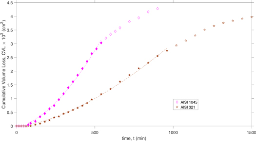
Figure 9. ICET cumulative volume loss of AISI 1045 and AISI 321 (ICET BAS data). Filled markers represent the data region utilized for model fitting. Dotted lines are three parameter HPM fits.
Download figure:
Standard image High-resolution image
Table 5. ICET HPM fit parameters.
| Epg (kJ · mol−1) | k (cm · min−n) | n | |
|---|---|---|---|
| Al 5052 | −24.3 | 9.18 × 10⁻⁴ | 0.18 |
| CuZn37 | −21.3 | 5.56 × 10⁻⁴ | 0.21 |
| Iron | −29.1 | 7.83 × 10⁻⁵ | 0.35 |
| AISI 1045 | −28.2 | 8.37 × 10⁻⁵ | 0.23 |
| AISI 321 | −35.5 | 2.62 × 10⁻⁵ | 0.20 |
Similar to the experimental results presented earlier, the ICET results exhibited differences in the cumulative volume loss values for the five metals. For the three metals presented in figure 8 there is a discernable difference between Al 5052 relative to CuZn37 and Iron. It is difficult to predict whether Al 5052 or CuZn37 would exhibit larger cumulative volume loss values using yield strengths or hardnesses of these alloys alone. Once again, the crystal structures of the three metals may explain the observed trend. Al 5052 is FCC, CuZn37 is a duplex brass containing both FCC and body-centered cubic (BCC) phases, and iron is BCC. As with our own data, the FCC metal exhibits the highest cumulative volume loss whereas the BCC metal exhibits the lowest.
For the two metals presented in figure 9 there is a discernable difference in the cumulative volume loss between AISI 1045 and AISI 321 that does not correlate with material properties (table 6). As before, alloy crystal structure provides a better explanation of the cumulative volume loss results. AISI 321 is an austenitic steel with FCC structure. AISI 1045 is a carbon steel composed mostly of martensite (highly-strained body centered tetragonal) with small amounts of ferrite (FCC) and pearlite phases. Pearlite is a lamellar microstructure consisting of alternating ferrite and cementite (orthorhombic). One would again expect the FCC metal to exhibit a higher rate of material loss due to ductile rupture than the non-FCC alloy. AISI 1045 exhibits a lower rate of material loss than CuZn37 or Iron because it has significantly higher hardness and yield strength.
Table 6. Material properties of ICET metals [15].
| Metal | Ultimate tensile strength, σUTS (MPa) | Yield strength, σy (MPa) | Elastic modulus, E (GPa) | Hardness (vickers) |
|---|---|---|---|---|
| Al 5052 | 208 | 169 | 70 | 71.7 |
| CuZn37 | 352 | 117 | 99 | 80.9 |
| Iron | 328 | 263 | 210 | 108.4 |
| AISI 1045 | 721 | 419 | 210 | 192.8 |
| AISI 321 | 605 | 225 | 200 | 191.0 |
Comparison of the three parameters obtained for Al 5052 and CuZn37 with those for the two closest metals used in our studies as listed in table 2—Al 6061 and Cu 110—shows reasonable agreement for all three parameters. The Hemispherical Pit Model is thus able to fit both new experimental cumulative volume loss data and historical cumulative volume loss data from comparable ICET cavitation erosion studies. Not only is the HPM applicable to metals of a variety of crystal structures and material properties, but it is based on a simple geometric description of an activated process—namely the uniform growth of surface pits after rapid pit formation—with parameters related to activation energy for pit growth (Epg), rate of pit growth (k) and time (n). How these parameters correlate with material properties beyond crystal structure, and how widely applicable the HPM is to non-metallic and non-crystalline materials are the subjects of future investigations. Also the subject of further investigation is the implicit prediction that as an activated process, temperature will influence the rate at which pits grow, thereby affecting the cumulative volume loss. Future experiments will include careful estimations of the number of pits, N.
5. Conclusions
The Hemispherical Pit Model shows excellent agreement, goodness of fit R2 greater than 0.99, with the cumulative volume loss of Al 6061, Cu 110, and Zn for sonication times up to 120 min at temperatures of 43 °C and 86 °C. The model parameters consist of the energy of pit growth, Epg, the rate of growth of the pit radius, k, and a time exponent, n. The ranges of these fit parameters are −22.1 to −29.0 kJ · mol−1, 2.49 × 10⁻⁴ to 9.12 × 10⁻⁴ cm · min−n, and 0.07 to 0.34, respectively. Compared to the Hattori and Szkodo models, the HPM is based upon a simple geometrical model of the volume loss process and contains parameters that may be more directly related to material properties. Additionally, the HPM shows excellent agreement with the growth regions of the erosion data obtained by the Bulgarian Academy of Sciences (BAS) for the International Cavitation Erosion Test (ICET).
Competing interests statement
No competing interests existed in this study.
Financial statement
Financial support was provided by the Carol Lavin Bernick Faculty Grant program at Tulane University.