
Abstract
The thermally activated, incoherent hopping of small electron polarons generated by continuous illumination in iron-doped lithium niobate is simulated by a Marcus-Holstein model for which all the input parameters are known from literature. The results of the calculations are compared with a comprehensive set of data obtained from photorefractive, photogalvanic and photoconductive measurements under green light excitation on samples with different doping levels and stoichiometries in the temperature range between  and room temperature. We show that the temperature and composition dependence of the photorefractive observables can be interpreted by a change in the abundance of the different hop types that a polaron performs before being captured by a deep Fe trap. Moreover, by a comparison between experimental and numerical data we obtain new insights on the initial photo-excitation part of the photorefractive process. In particular all results are consistent if a single value of the photogalvanic length
  is assumed for all the samples and all the temperatures. The photo-generation efficiency ϕ under green light excitation (somewhere denoted as quantum efficiency) is also estimated. It appears to decrease from 10%–15% at room temperature to about 5% at 150 K. This behavior is qualitatively interpreted in terms of a temperature-dependent re-trapping probability of the light-emitted particles from the initial Fe donor center.
Export citation and abstract BibTeX RIS

Original content from this work may be used under the terms of the Creative Commons Attribution 3.0 licence. Any further distribution of this work must maintain attribution to the author(s) and the title of the work, journal citation and DOI.
1. Introduction
Lithium niobate (LiNbO3, LN) is often taken as a paradigm for light induced charge transport phenomena in polar oxide crystals. This is the physical basis of the so-called photorefractive effect, which in LN is especially strong as a consequence of the high electro-optic coefficients and of the fact that large internal electric fields (106 − 107 V m−1) can be built up in the bulk simply by illuminating this material with visible low intensity light [1]. Those phenomena bear a high interest for practical applications: in the field of non-linear and ultra-fast optics the photorefractive effect limits the use of LN for high intensity processes [2], while in photorefractive holography it is used to record high quality gratings, optical memories and demonstrate low-intensity all-optical interactions [3]. Integrated optics as well needs to control those phenomena due to the high cw light intensities obtained in wave-guiding regions [4]. In more recent approaches, the space charge field was exploited to manipulate nano-sized materials [5] or to operate liquid-crystal photorefractive cells [6]. Additionally, the exploding field of ferroelectric photovoltaics has attracted a strong interest in understanding charge transport processes in polar materials [7].
The microscopic origin of those internal electric fields is related to the interplay between the photogalvanic effect (i.e. the appearance of a bulk current density proportional to the photon flux) and the charge transport mechanisms that determine the material conduction [8]. Both those phenomena have been described in the past by mutuating from semiconductor physics a band model picture embodied by the well-known Kukhtarev-Vinetskii equations [9].
However, more recently, charge transport phenomena in LN:Fe has been interpreted in terms of small polarons creation and migration [10]. In the initial stage of the process, some charge carriers are photo-generated from deep donor centers and emitted with a preferential direction in the conduction band. Subsequently those 'hot' carriers lose energy by interaction with the lattice and finally condensate into a new state which is self-localized by a distortion of the local ionic environment. Under certain conditions the carrier, localized at a single lattice site, and the surrounding deformation can be thought as a quasi-particle that moves as a whole: the small polaron. Its motion takes place by thermally assisted hopping transitions to adjacent sites [11]. It is therefore mandatory to update the description of light—induced charge transport phenomena incorporating the polaron physics.
In Fe:LN the initial step of the photo—transport process relies on poorly known phenomenological parameters: the photogalvanic length LPG and the photo-generation efficiency ϕ (sometimes indicated also as quantum efficiency). The former can be interpreted as the average position from the donor center at which a newly emitted charge condensates into a polaron. The fact that this average is different from zero in absence of an applied field is the very origin of the photogalvanic effect. The second parameter ϕ indicates that not all the absorbed photons succeed in creating a polaron contributing to the photogalvanic effect.
On the other hand, the second step of the photo—transport process, i.e. the incoherent hopping transport of small polarons, can be modeled by means of the Marcus-Holstein model [12, 13]. It has been shown [14] that by using few parameters obtainable from spectroscopic measurements this model can successfully reproduce the polaron transport in a wide composition and temperature range by means of Monte Carlo simulations dealing with the different polaronic centers present in LN:Fe.
The aim of the present work is therefore to compare experimental data obtained on a set of samples with different compositions and between room temperature and 150 K with Monte Carlo simulations based on the Marcus-Holstein hopping model. From the comparison a quantitative estimation of LPG and ϕ will be obtained, as well as some insights on how the observed dependencies can be interpreted in terms of polaron hopping.
2. Experimental
2.1. Macroscopic observables
In the following we consider the simplest experimental situation of a Fe:LN sample illuminated with a uniform strip of light (see figure 1). The c axis is supposed to be parallel to the input surface and perpendicular to the illuminated strip, to realize a quasi 1-D configuration. In these conditions a refractive index change is observed as a consequence of the buildup of a light-induced space charge field and of the electro-optic effect [3, 15]. Thus, the main quantities of interest in describing the photo—transport in Fe:LN are essentially three: (i) the photogalvanic current initiating the buildup of the field; (ii) the material's conductivity under illumination; (iii) the stationary space charge field, proportional to the maximum refractive index change. Those quantities will be briefly discussed in the next sessions in the context of polaron transport. We developed an all-optical setup, described in the Supporting Information, which allow for a measure of those three quantities without the need for electrical connections and as a function of temperature. The macroscopic observables were then systematically measured on a set of six samples presented in forthcoming paragraphs.
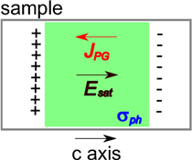
Figure 1. Scheme of the experimental geometry: a Fe:LN sample is illuminated with a uniform strip of light. Inside the illuminated volume a current density jPG and a conductivity σPC are established. The charge accumulation at the boundaries of the illuminated area give rise to an electric field Esat that in stationary conditions counterbalances the photogalvanic current.
Download figure:
Standard image High-resolution image2.1.1. Photogalvanic current
In the case of the 1D problem described above, the photogalvanic current is directed essentially along the c axis and can be written in scalar form [1, 10] as:

where q is the charge of the photo-excited carriers, α = sN is the absorption coefficient (with s the cross section and N the concentration of the photogalvanic centres, respectively), I is the light intensity, hν the photon energy and LPG the photogalvanic length. ϕ is the photo-generation efficiency factor, i.e. the probability to create a charge contributing to the current from an absorbed photon, appearing also in the expression for the photoconductivity (see next section). Since all the parameters involved in the photo-generation rate  are known, it is convenient to normalize the experimentally measured jPG with respect to G, obtaining what we may call the effective photogalvanic length:

It should be noted that usual experiments provide access to this quantity, but not to ϕ and LPG separately.
2.1.2. Photoconductivity
The photoconductivity σph is generally expressed [3] as:

In this equation μ is the drift mobility of the light—induced carriers, n their concentration and τ their lifetime. The last equivalence is derived from a band-like description using a rate-equation system [3]. It is important to note that this expression requires two fundamental assumptions (i) the charge carriers are normally diffusing particles characterized by a time-independent mobility; (ii) the carrier decay time is described by an equation of the kind  , where N+ is the concentration of ionized donors acting also as deep traps, [Fe3+] in our case. Both those assumptions are fully reasonable in a band model, but when dealing with polaron transport they need more careful verification. Normal diffusion laws may not be verified [16] for a polaron hopping on a defective lattice with a distance- and energy- dependent attempt frequency. On the other hand, a rate equation such as the one used in band models entails the mono-exponential decay of a carrier population, while it is known (see e.g. [2]) that polaron decays are rather described by stretched exponential functions (Kohlrausch—Williams- Watts law) owing to a heavy-tailed distribution of trapping times.
Those observations indicate that in the polaron context it is challenging knowing or even defining μ and τ separately. However, as already observed by Sturman et al [17], the above mentioned problems can be overcome considering that what is needed here is not μ, nor τ in isolation but the quantity that in a band model is given by the product μτ i.e. the average distance  run by a polaron under a unitary electric field from its creation to its trapping. Differently from μ and τ in isolation, this quantity can be operatively defined also in our context:

and can be straightforwardly computed by a Monte Carlo approach. It should be noted that the  displacement of a hopping particle under electric field and after a given time remains proportional to the electric field magnitude under very general conditions, including anomalously diffusing particles [16] so that the definition is robust.
The photoconductivity (normalized for the photo-generation rate G) is thus given in terms of Λ:

2.1.3. Space charge field
Under homogeneous cw-light exposure, charge carriers tend to move along the c axis due to the photogalvanic effect. Charge accumulation outside illuminated areas gives rise to the build-up of a space charge field in the material. Assuming that diffusion currents and dark conductivity are negligible, as it is appropriate in the experimental conditions adopted in this work, the saturation value of the electric field Esat is attained when, after an initial transient, the photogalvanic current, equation (1), is counterbalanced by the drift current jdrift = σphE. From equations (1), (3) one has:

The initial transient of the space charge field evolution, for our simple 1D geometry, follows a simple exponential law [3, 15]:

The time constant τd in equation (7) is the so-called dielectric relaxation time, given by:

and provides a direct access to the sample photoconductivity σph.
2.2. Samples
Two series samples were grown for this work. The first one is composed of congruent samples ( ratio equal to 0.94) but with different iron concentrations (Series sample A), grown by Czochralski technique at the University of Padova (Italy). This series of samples is conceived to study the effect of different trap concentrations. The Fe contents in the melt was chosen equal to
  ,
,  and
and  . The second sample series (referred as B) is the one having a fixed deep trap concentration but a different amount of shallow traps (i.e. niobium antisites). In particular three samples, doped with Fe
  , with different stoichiometry were grown at the Institute for Physical Research in Ashtarak (Armenia). High-purity compounds of
  from Johnson-Mattley, and
  from Merck, in powder form, were used as the starting materials for sintering of the lithium niobate charges of different composition, via solid state reaction. The appropriate amount of iron was added to the initial charges of LN in the form of
  oxide (Merck) and thoroughly mixed. This kind of growth is known to produce samples with a composition which is not constant along the growth direction. Therefore the precise composition of the final samples cannot be assumed to be equal to the one of the melt and needs to be characterized. All the samples were x-ray oriented, cut and optically polished in parallelepipeds with typical sizes of some millimeters per side.
The  absolute concentration is obtained from the optical absorption at
  as proposed by Berben et al [18]. Assuming that, for weak doping levels as the ones used here, the total Fe concentration in the crystals is the same as in the melt, the amount of Fe3+ traps present in the samples is obtained by difference. The concentration of NbLi antisite defect can be estimated by Raman spectroscopy [19–21] since a linear relationship between the Li deficiency and the broadening of Raman peaks was established. All the samples of the series B were measured in the X(zz)X backscattering configuration using a LabRAM Aramis Micro-Raman spectrometer, in order to obtain the
  modes, corresponding to
  vibrations in x-cut samples [22]. The modes were fitted by Lorentzian functions in order to measure their FWHM Γ and from the equation [21]:

the molar concentration ![${X}_{C}=\tfrac{[{Li}]}{[{Li}]+[{Nb}]}$](https://content.cld.iop.org/journals/2399-6528/2/12/125003/revision2/jpcoaaf3ecieqn19.gif) can be obtained. However, in this work a different instrument with respect to the one mentioned in [21] was used, so the formula 9 has to be checked. The spectral line profile used in this analysis is Lorentzian which width is due to the 'true' Raman line shape convoluted with a 'instrumental' function, which depends on the instrument used, on the wavelength etc. As the convolution of two Lorentzian functions is again a Lorentzian whose width is equal to the sum of the widths of the two functions, it can be considered that a change in the setup may affect only the intercept of equation (9), while the slope may be considered as accurate. To estimate the correct intercept, a reference sample is needed. The congruent composition is by definition the one in which the crystal composition is equal to the melt composition and can be expected to be the one with the highest compositional uniformity. In the following therefore the samples grown from the congruent melt are considered as reference and their composition is assumed by default.
can be obtained. However, in this work a different instrument with respect to the one mentioned in [21] was used, so the formula 9 has to be checked. The spectral line profile used in this analysis is Lorentzian which width is due to the 'true' Raman line shape convoluted with a 'instrumental' function, which depends on the instrument used, on the wavelength etc. As the convolution of two Lorentzian functions is again a Lorentzian whose width is equal to the sum of the widths of the two functions, it can be considered that a change in the setup may affect only the intercept of equation (9), while the slope may be considered as accurate. To estimate the correct intercept, a reference sample is needed. The congruent composition is by definition the one in which the crystal composition is equal to the melt composition and can be expected to be the one with the highest compositional uniformity. In the following therefore the samples grown from the congruent melt are considered as reference and their composition is assumed by default.
The results of those characterizations are reported in table 1. In the following, to indicate a sample we adopt the labelling convention: Series/Deep Traps (in  )/Shallow Traps (in
  ). Thus for example, the label A/0.34/19.0 indicates the sample of the series A with a Fe3+ concentration of
  and a
and a  antisite defect content of
  .
.
Table 1.
Summary of compositional parameters for the two groups of samples investigated. In the last column the reduction ratio ![$R=[{\mathrm{Fe}}^{2+}]/[{\mathrm{Fe}}^{3+}]$](https://content.cld.iop.org/journals/2399-6528/2/12/125003/revision2/jpcoaaf3ecieqn25.gif) is also reported.
is also reported.
| Sample name | XC% |
![$[{\mathrm{Nb}}_{{Li}}]$](https://content.cld.iop.org/journals/2399-6528/2/12/125003/revision2/jpcoaaf3ecieqn26.gif)
|
![$[{\mathrm{Fe}}_{{tot}}]$](https://content.cld.iop.org/journals/2399-6528/2/12/125003/revision2/jpcoaaf3ecieqn27.gif)
|
![$[{\mathrm{Fe}}^{2+}]$](https://content.cld.iop.org/journals/2399-6528/2/12/125003/revision2/jpcoaaf3ecieqn28.gif)
|
![$[{\mathrm{Fe}}^{3+}]$](https://content.cld.iop.org/journals/2399-6528/2/12/125003/revision2/jpcoaaf3ecieqn29.gif)
|
R% |
|---|---|---|---|---|---|---|

|

|

|

|
|||
| A/0.34/19.0 | 48.45 | 19.0 | 0.37 | 0.04 ± 0.01 | 0.34 ± 0.1 | 10.9 ± 0.3 |
| A/0.82/19.0 | 48.45 | 19.0 | 0.95 | 0.12 ± 0.01 | 0.82 ± 0.02 | 14.3 ± 0.3 |
| A/1.56/19.0 | 48.45 | 19.0 | 1.89 | 0.33 ± 0.01 | 1.56 ± 0.07 | 21.1 ± 0.4 |
| B/1.84/19.0 | 48.45 | 19.0 | 20.9 | 0.24 ± 0.01 | 1.84 ± 0.01 | 13.08 ± 0.09 |
| B/1.78/17.5 | 48.58 ± 0.03 | 17.5 | 20.9 | 0.31 ± 0.01 | 1.78 ± 0.05 | 17.2 ± 0.5 |
| B/1.94/6.4 | 49.49 ± 0.03 | 6.4 | 20.9 | 0.15 ± 0.01 | 1.94 ± 0.02 | 7.6 ± 0.1 |
3. Theory and simulation
3.1. Microscopic model
LN hosts four different kinds of intrinsic small polarons [23]: the free polaron (FP)  , the bound polaron (GP)
  , the bipolaron (BP)
  , and the hole polaron (HP)
  . Electrons bound to
  may also be described in the framework of the strong-coupling-polaron picture. Hole polarons are produced at visible wavelengths by high intensity pulsed beams by two-photon processes and will not be considered here, as in our Fe doped samples and at cw intensities the electron generation from Fe2+ is by far predominant. Moreover, in Fe-doped samples, bipolarons are not observed because the system tends to relax to the more stable Fe defect, so in the following we will disregard also this centre. In conclusion, we will assume that in the dark the sample does not contain free or bound polarons and that all the charges are stored in Fe2+ centres. When a photon in the visible range is absorbed by a Fe2+ donor, a small electron polaron is created. It performs a certain number of hops either on NbNb or on NbLi sites until it is re-trapped at a deep
  trap, which defines the final distance run by the particle.
3.2. Polaron transport in Fe:LN
According to the Marcus—Holstein polaron hopping model [11–13], the non-adiabatic hopping frequency for a ( ) hop is:

In equation (10), r is the distance between initial and final sites and kT the absolute temperature (in energy units). λi,f is the reorganization energy of Marcus' theory corresponding to the energy paid to rearrange the lattice, here equal to  , sum of the elastic energies of the two polarons; ai,f is an orbital parameter describing the overlap between the electronic wave functions at site i and f. The 1/2 factor is due to the fact that equation (10) expresses the individual rate to a given final site, and is thus one half of the total rate in Holstein's molecular chain [13].
  is the hopping barrier, given by [24, 25]:

with εi and εf the pre-localization energies of the electron at zero deformation. When the hop occurs between sites of the same type (i = f), Ui,i = Ei/2, recovering the standard result that the hopping activation energy is one half of the polaron energy [2, 23, 26]. The pre-exponential factor Ii,f describes the intrinsic hopping rate between the two sites and is determined by the choice of the (i, f) combination. According to this model, each of the three centers here considered (two Nb- based polarons, NbLi and NbNb and the  defect) and the hopping combinations between them are described by a set of parameters. According to some recent results [14], the parameters choice reported in table 2 provides a fair description of all the possible hopping processes in Fe:LN, and will be used throughout this work.
Table 2. Parameters used for the simulation (see text).
| Parameter | Value | Unit | References | Note |
|---|---|---|---|---|
| EFP | 0.545 | eV | [23] | Free polaron energy |
| EGP | 0.75 | eV | [14] | Bound polaron energy |

|
0.7 | eV | [23] | Fe defect energy |

|
0 | eV | Free polaron pre-localization energy | |

|
0.2 | eV | [14] | Bound polaron pre-localization energy |

|
1.22 | eV | [23] | Fe defect pre-localization energy |

|
1.6 | Å | [14] | Hopping parameter |
|
1.3 | Å | [14] | Trapping parameter |

|
0.1 | eV | [27] | Transfer integral pre-factor |
The effect of the space-charge field E on the hopping frequency is described by adding in equation (11) the term  inside the parenthesis at the numerator, with ri(j) the position vectors of the starting (final) site. It is important that the field is not too strong to maintain the character of random diffusion in our simulation. In other words, the potential energy
  gained by the polaron must remain small with respect to kT. Our field is therefore set at
  for all the temperatures, a compromise between the above -mentioned requirement and the necessity to observe a measurable displacement. The field is directed along the crystallographic c direction to mimic our experimental geometry.
It should be recalled that the hopping formula (10) is valid only in the non-adiabatic approximation [11] which holds whenever the transfer integral  is much smaller than the reorganization energy
  . By using the values reported in table 2 we can check that this condition is well satisfied for all the hop types considered in our model. Moreover the approximation requires the lattice to possesses sufficient thermal energy to follow the charge motion and, as a rule of thumbs, is considered safe for temperatures above
  where
where  is the Debye temperature for lithium niobate [28]. However, experimental results obtained by Faust et al [29] show that the the Arrhenius behaviour of the mobility in antisite-free LN is preserved till
  , indicating that the non-adiabatic approximation in LN holds at least down to this temperature.
3.3. Monte Carlo simulation
The simplest numerical approach consists in simulating one single electron at time. This situation corresponds to a low electron density system where interaction between electrons can be ignored. The electron, randomly placed at an initial NbNb site, performs a walk in a structure reproducing the LN lattice. The code generates a random defect configuration in a 80 × 80 × 80 super-cell of the LN structure with periodic boundary conditions, in which the polaron is launched and the position at which it is captured by a Fe3+ trap is recorded. The different defect concentrations of the various samples are set in accordance with table 1. The code computes the rest time on each visited site and the next destination site according to equations (10), (11) by a classical Gillespie algorithm, as explained in [25]. The probability to hop from a site i to a site f is computed as:

where the summation at the denominator goes on all the possible destination sites inside a suitably defined volume surrounding the starting site. The simulation is repeated for a sufficient number of times, in order to compute the average distance  along the field direction run by the particles before being captured. From equation (4) the value of Λ is calculated for the different samples and for all the experimental temperatures.
4. Results
4.1. Space charge field and photogalvanic length
In figures 2(a), (c) are reported the experimental results (dots) for the saturation space charge field value Esat as a function of temperature for sample series A and B. The field shows a monotonous increase by decreasing the temperature.

Figure 2. (a) Saturation space charge field as a function of temperature for sample series A. Dots: experimental points; Lines: recomputed results taking  and
and  (see text for details). (b) Simulated Λ for sample series A. (c) Same as (a) for sample series B. (d) recomputed Λ for sample series B.
Download figure:
Standard image High-resolution imageThe central result of our simulation is the drift coefficient Λ, i.e. the mean distance covered by a polaron under a unitary electric field from its birth to its trapping. In figures 2(b), (d) the simulation results obtained in the same conditions as in (a), (c) are shown. The Λ value becomes smaller and smaller by decreasing the temperature, indicating that at low T the polaron is able to cover on average a smaller distance. By increasing the trap concentration in sample series A, Λ is decreased as well, as it can be expected (figure 2(b)). The effect of the antisite concentration in sample series B (2(c)) is somehow less evident, due to the high Fe concentration that in the temperature range here explored keeps always Λ below  (note the different ranges in the ordinates of (b) and (c)). However a trend is visible indicating that a higher antisite concentration hinders the charge motion or, conversely, by increasing the Li content towards stoichiometry Λ is increased.
In figure 3 is shown the correlation plot between the reciprocal of the measured saturation space charge field 1/Esat and the Λ values simulated for the corresponding experimental conditions. A linear correlation is recovered for almost all the samples, as it can be expected by the reciprocal of equation (6),  , and by the observation that LPG is an intrinsic parameter of the Fe:LN system which should be almost independent from temperature and composition [10]. Thus, the fact that almost all our data converge on a unique line can be considered as a self-consistency test. However a nonzero Λ0/LPG intercept is clearly evident from the graph. This can be interpreted as a parasitic contribution to the sample conductivity. Since this contribution appears to add up to to all the samples and for all the temperatures, this feature is likely to be an extrinsic contribution e.g. some unwanted leakage perhaps facilitated by the contact with the metallic sample holder inside our cryostat system. We note here, however, that few points relatives to the sample A/0.34/19.0 at high temperatures appear to deviate from the linear behaviour. Our data do not allow at the moment deciding whether this is an artifact or the indication that in a range of experimental conditions wider than the one here considered the description becomes more complicated. As the large majority of our data is in agreement with the simple description of equation (6), we will stick here to this model, with the caveat that further work is needed to confirm their validity out of the conditions here explored.

Figure 3. Correlation plot of experimental 1/Esat values against simulated Λ for all the measurements. The red line is a linear fit of the data.
Download figure:
Standard image High-resolution imageFrom the linear fit of figure 3 we retrieve  and
and  . From those values and from the results of the simulations, the saturation space charge field was re-computed by equation (6) for all the experimental conditions here examined and reported in figures 2(a) and (c) as solid lines. To our knowledge, this is the first direct comparison between temperature- and composition- dependent data in photorefractive Fe:LN and the calculations obtained from a microscopic polaron model in which no free parameters besides LPG and
  were used.
4.2. Photoconductivity and photo-generation efficiency
In figures 4(a) and (c) are reported the experimental values of the specific photoconductivity Σ (dots). Combining them with the determination of LPG and from the measured values of Esat it is possible to estimate the photo-generation efficiency ϕ as a function of temperature. In fact, from equations (2), (5), (6) one gets easily  . The results are reported in figures 4(b) and (d). All the data are coherent among the different samples: ϕ appears to decrease by cooling the sample from a value of 10%–15% at room temperature to about 5% at low T.

Figure 4. (a) Experimental results (dots) for the specific photoconductivity Σ for sample series A. By comparison the values obtained from our simulation corrected for the empirical values of ϕ and Λ0 are shown (broken lines). (b) Photogeneration efficiency ϕ for the sample series A. (c) Experimental results (dots) for the specific photoconductivity Σ for sample serie B. By comparison the values obtained from our simulation corrected for the empirical values of ϕ and Λ0 are shown (broken lines). (d) Photogeneration efficiency for sample serie B.
Download figure:
Standard image High-resolution imageBy comparison, we recompute Σ according to equation (5) using the obtained values of ϕ, the simulated values for Λ and the correction for the leakage Λ0, i.e.  . The results are plotted in figures 4(a) and (c) as solid lines, showing that again all the description is consistent.
5. Discussion
5.1. Drift Coefficient
The interpretation in terms of polaron hopping of the temperature and composition dependence of the photorefractive phenomena opens up a rich scenario, in which the interplay between the different defect centers determines the drift coefficient Λ and ultimately the main photorefractive observables.
Our simulation provides access to Λ. The decrease of this parameter with temperature (see figures 2(b), (d)) is due to the fact that, as a general rule, by decreasing the temperature the polarons perform a smaller number of hops to get trapped by a Fe ion [25]. It should be noted that in a hypothetical material with no NbLi antisites and vanishing Fe concentration this would not be the case. In this situation the only charge carriers would be free polarons performing a given number of hops before being trapped by a deep trap. The conduction would be ensured by thermally activated hopping among equal sites characterized by a single activation energy. Therefore the temperature term of the Marcus-Holstein frequency, equation (10), would be the same for all hopping processes and could be simplified out from equation (12). This proves that the random walk performed by the polaron in this case is not affected by temperature, which would only speed up or slow down the hopping frequency, but would not change the number of hops and the distance run under the field before being trapped. The situation is different for a material with defects. In this case the starting and destination sites may be of different kind so that the hopping barriers may not be the same for all the hopping processes. The thermal part of the hopping frequency therefore cannot be simplified in equation (12) which becomes temperature dependent. Therefore, in material containing defects a change in temperature, besides modifying the speed of the hopping process, influences also the random walk of the particle. In particular, at sufficiently low temperatures and for the Fe concentrations used in this work, the hopping frequency of the trapping processes  becomes dominant with respect to the others, leading to an increase of the trapping probability upon decreasing T.
For a given sample composition we may therefore distinguish two limiting hopping regimes, upon cooling down from room temperature (or above): (i) Multi-hop, mixed transport regime: the thermal budget is so high that all the hopping processes occur more or less frequently and the polaron performs several hops before being captured by a Fe3+ trap. In this regime the drift coefficient Λ depends strongly on the relative amount of the different hop types; in particular, at high temperatures and/or low antisite concentrations the free polaron jumps  dominate the transport [14]. (ii) Trapping regime: at sufficiently low temperatures, the hopping frequency towards Fe traps becomes higher than for all other processes, so that direct trapping becomes the most likely event. The two situations are illustrated in figure 5 where the average percentage of the different hop types over the total hop number has been computed from our simulation code for sample A/0.82/19.0 as an example.

Figure 5. Distribution of the different hop types as a function of temperature in congruent sample A/0.82/19.0 calculated using the parameters of table 2. Only transport ( and
and  ) and trapping (
 and
and  ) processes are reported, the others being inefficient 'conversions'
  in which the polaron jumps back and forth between the same sites.
Download figure:
Standard image High-resolution imageThe simulations show that in these conditions the trapping can occur even if the trap is quite far away from the newborn polaron, i.e. several tens of Angstroms. A useful way to visualize this process is the concept of trapping radius firstly introduced in [25]. The trapping probability can be estimated by comparing the hopping frequency towards the Fe donor against the frequency towards any other center. As the hopping frequency (equation (10)) depends both on distance and on temperature, one can ask what is the distance d(T) from a neighboring Fe center under which the polaron is more likely to be trapped than to hop away, for a given T. By some simple considerations detailed in [25], it turns out that this distance obeys an equation of this kind:

and increases from about 20 to  by decreasing T from room temperature to
  . The onset of the trapping regime can thus be visualized by imagining that each trap is surrounded by a finite 'capture volume' with a trapping radius that increases by cooling down the sample. At low T the trapping volumes start to fill most of the available space, so that the polarons are captured within few hops.
5.2. Photogalvanic length
Schirmer et al [10] gave a comprehensive revision of the photogalvanic effect in Fe:LN reinterpreting it within the polaron model. The initial direction along which the charge is emitted as a Bloch wave is determined by the Fermi golden rule, the different matrix elements of the transition being determined by the geometrical arrangement of the ions surrounding the donor centre. In this vision the photogalvanic length LPG in equation (1) corresponds to the averaging along the c-axis of the distance covered in the different directions prior to the polaron formation. The electron is supposed to move several NbNb − NbNb distances coherently along the c axis before the lattice relaxes around it to form a  small polaron state.
Our data show a consistency with the Marcus-Holstein model if a value of  is assumed. In accordance with microscopic considerations, this parameter appears to be independent on the sample and on the temperature for the range of experimental conditions explored in this work. The quantitative result is in reasonable agreement with previous tentative estimates [10] which gave LPG in the Angstrom range for Fe excitation with visible light. This value may be compared with the diffusion distance that a newly emitted 'hot' electron travels before condensate into a polaron, which is much larger and estimated around
  [10] on average. This means that the photo-excited charge is emitted nearly isotropically and that the nonzero average displacement is only a tiny fraction of the distance run by the electron wave before the self-localization.
5.3. Photogeneration efficiency
The results obtained on different samples are consistent between them and point out that ϕ is between 10 and 15% at room temperature and decrease to 5% at 150 K. In [30] it is reported that ϕ decreases of about 4 times by increasing the wavelength λ from the blue to the green. Since ϕ cannot be larger than 1, in our experiments with  we must have ϕ < 0.25, in accordance with our data.
According to the model for emission of photo-excited charges mentioned in the precedent paragraph, after the initial thermalization stage the polaron is formed at a certain distance from its donor site according to some probability distribution with a mean equal to LPG and a width of the order of  . The particle has now two possible choices to continue its life: to move away or to jump back to the same initial site it came from, both processes being thermally activated but with a different energy barrier. This provides a microscopic interpretation for the parameter ϕ introduced in equation (1), which denotes here the probability for the polaron to not go back to the starting site [31]. As explained above, at low temperature the trapping become more efficient and this can be visualized by considering that the trapping radius R(T) of the Fe centers increases at low T. The trapping radius is of the order of
  at room temperature, i.e. of the same order of magnitude of the diffusion distance of the hot polaron. The low value of the photo-generation efficiency is therefore explained by the fact that a large part of the polarons are formed inside the trapping radius and are thus recaptured by the same Fe donor they came from (see figure 6).

Figure 6. Proposed scheme for the interpretation of the photogeneration efficiency. The grey circle represents the volume where the newly formed polarons are likely to be retrapped by the Fe donor. The polarons can form at any distance from the donor center with a given probability distribution (see text).
Download figure:
Standard image High-resolution image
The effect of the temperature can be easily understood as the trapping radius increases by lowering T, as a consequence of the temperature dependence of the hopping frequencies, so that the chance to escape is smaller and smaller. The increase of the photo-generation efficiency with the wavelength reported in [30] can be easily interpreted in this framework as well, considering that more energetic photons are able to project the photo-emitted charge at a longer distance from the Fe center [10]. It would be interesting to push this analysis to a more quantitative modeling, but for this aim it would be necessary to know the probability distribution function for the formation site of the polarons around the donor center. Further work is in progress to investigate this idea.
6. Conclusions
The charge transport processes inherent to photorefractivity in Fe:LN are of two kinds: the first is the coherent motion as a conduction band state of a newly emitted charge upon absorption of a photon. The second is the localization of the charge at a single lattice site and its incoherent hopping among regular and/or defective sites. In this work we modeled the second part of the process by means of a Marcus-Holstein hopping model, in which all the parameters were fixed by a priori known parameters. This allow us to calculate explicitly the incoherent transport without any assumption.
In parallel, by means of a dedicated experimental setup and tailored samples, we collected a comprehensive set of data on the photogalvanic, photoconductive and photorefractive properties as a function of the sample composition and in the temperature range between 150 K and room temperature to test the model previsions.
We showed that the experimental data and the numerical simulations are consistent with each other if a value of  independent on the temperature and on the composition is assumed for the photogalvanic length, i.e. the average distance from the donor center at which the photo-emitted charges localize into a polaron. Moreover, by comparison with photoconductivity data, we can obtain an estimate for the photo-generation probability ϕ for Fe2+under green light excitation, which amounts to about 10% at room temperature, decreasing to 5% at 150 K. Both those quantities appear to be independent on the sample composition within our experimental accuracy and for the conditions here reported. This is, to our knowledge, the first direct quantitative estimation of those parameters related to the photo-generation process. The obtained values are in line with previous heuristic estimations reported in literature. It should be noted that the Marcus-Holstein analysis here validated for the wavelength of
  could be extended to obtain information for other wavelengths, helping to investigate the dependence of the LPG and ϕ upon the photon energy. Further work is needed to verify those findings for higher transport lengths.
Besides those quantitative results, our analysis provides an interpretation of the observed dependencies in the framework of the polaron model. In particular it was found that, as a general rule, by cooling the sample (for a given trap density) the number of hops and the distance run by the particle under an electric field decrease. This phenomenon, not explained by standard formulation of photorefractive equations, is a direct consequence of the combined temperature/distance dependence of the Marcus-Holstein frequency, which favors at low temperature hopping transitions towards distant Fe traps. It turns out that at sufficiently low T, the largest part of the photo-excited carriers are all trapped within few hops, entering what we may denote as 'trapping' regime as opposed to the 'multi-hop' regime at high temperatures. The same phenomenon accounts for the observed decrease of the photogeneration probability ϕ with T. In this respect, ϕ is thus interpreted as the complementary of the probability that the photo-induced charge is recaptured by the same Fe donor which it came from.
Lastly, we stress how the Marcus-Holstein model was proven to possess the capability to predict the photorefractive properties of Fe:LN starting from microscopic parameters that were obtained from optical absorption and pump-probe transient absorption spectroscopy [14, 23]. In principle the same predictive capability could be used to preview the photorefractive behavior of any dopant in a given concentration and even in presence of a co-dopant, once that the microscopic parameters of the new impurities are tuned by means of few targeted experiments. This would provide a powerful tool for crystal growers helping to design new crystal compositions with tailored properties, without undergoing the time-consuming process of synthesis and testing of a large number of samples.
Acknowledgments
This research was funded by the University of Padova, grant number BIRD174398. LV and MB acknowledge Dr N Argiolas and L Bacci at the University of Padova for invaluable technical assistance as well as the CloudVeneto infrastructure for providing the necessary resources for numerical simulations.