

Abstract
The aim of the MOCAST+ (MOnitoring mass variations by Cold Atom Sensors and Time measures) project, which was carried out during the years 2020–2022, was the investigation of the performance of a gravity field mission based on the integration of atomic clocks and cold atom interferometers. The idea was that the combined observations of the two sensors would be beneficial for the detection and monitoring of geophysical phenomena which have an impact on the time-variable part of the Earth gravity field models. Several different mission scenarios were simulated, considering different satellite configurations such as a Gravity Recovery and Climate Experiment (GRACE)-class formation and a Bender-class formation with either two or three in-line satellites along each orbit. Moreover, different atomic species (rubidium and strontium), different inter-satellite distances, different noise power spectral densities, and different observation rates were taken into account. For the gravity field estimation from the simulated data, the space-wise approach was exploited. The results showed that, as it could be expected, the Bender configuration provides significantly better monthly gravity field solutions, as compared to a 'nominal' configuration with two or three satellites in a GRACE-class formation. In this way, and pushing the quantum sensors technology to its limits, it is in fact possible to obtain results which are comparable with those from GRACE at low harmonic degrees, and are better at higher degrees with positive effects in the detectability of localized time variable phenomena, as well as in the determination of the static gravity field at a higher maximum spherical harmonic degree than the one achieved by Gravity Field and Steady-State Ocean Circulation Explorer (of course considering an equivalent mission life-time).
Export citation and abstract BibTeX RIS
1. Introduction and the MOCAST+ mission concept
The internal structure (crust, mantle and core activities) and external dynamics (rapid and long-term changes in atmosphere, ocean, ice, ground water) of the Earth causes mass variations in time, which have an effect on the gravity field and on its variations in time. In the past 20 years, thanks to missions like GRACE (Gravity Recovery and Climate Experiment) (Tapley and Reigber 2001, Kvas et al
2019) and GRACE-FO (follow on) (Kornfeld et al
2019, Landerer et al
2020), the scientific community had the possibility to exploit satellite data to model the temporal variations of geophysical processes. As a consequence, there has been a lot of progress in the monitoring of ice mass loss (Chen et al
2008, Velicogna 2009, Khan et al
2010), sea-level rise (Cazenave et al
2009, Leuliette and Miller 2009, Jacob et al
2012), ocean bottom pressure variations (Johnson and Chambers 2013), glaciers (Ciracì et al
2020), ground-water storage (Rodell et al
2007, Chen et al
2016, Xiang et al
2016, Fatolazadeh et al
2020), tectonic movements, and other solid Earth activities (Han et al
2006, Chen et al
2007, Wang et al
2012, Eshagh et al
2020). In the same decades, with the launch and completion of the successful GOCE mission (Gravity Field and Steady-State Ocean Circulation Explorer) (Drinkwater et al
2003), the static gravity field was estimated from satellite data with an unprecedented global spatial resolution of about 100 km (corresponding to spherical harmonic degree of about 200) and accuracy of  1 mGal in terms of gravity anomaly (Pail et al
2011). This mission was based on the observation of gravity gradients and gave the possibility to investigate the relationship between the gravity signal and different geophysical signals, leading to significant improvements especially in solid Earth monitoring and oceanography (see e.g. van der Meijde et al
2015). In particular, promising results were obtained in monitoring the mean geostrophic current in ocean circulation (Knudsen et al
2011), and in understanding the physics of the Earth interior structure, including the geodynamics linked to lithosphere, uplifting, post-glacial rebound and subduction processes (Tenze et al
2014, Bouman et al
2015, Braitenberg 2015, Reguzzoni and Sampietro 2015, Eshagh et al
2016, 2018, Reguzzoni et al
2019).
1 mGal in terms of gravity anomaly (Pail et al
2011). This mission was based on the observation of gravity gradients and gave the possibility to investigate the relationship between the gravity signal and different geophysical signals, leading to significant improvements especially in solid Earth monitoring and oceanography (see e.g. van der Meijde et al
2015). In particular, promising results were obtained in monitoring the mean geostrophic current in ocean circulation (Knudsen et al
2011), and in understanding the physics of the Earth interior structure, including the geodynamics linked to lithosphere, uplifting, post-glacial rebound and subduction processes (Tenze et al
2014, Bouman et al
2015, Braitenberg 2015, Reguzzoni and Sampietro 2015, Eshagh et al
2016, 2018, Reguzzoni et al
2019).
All the above-cited studies were the result of increased spatial (GOCE) and temporal (GRACE, GRACE-FO) resolution in the observations delivered by these missions. Yet, the scientific need for a more detailed modelling of geophysical processes requires an even higher spatial and temporal resolution, which is hardly achievable by exploiting the technology used in these missions, due to limits of the measuring instruments. As an example, let us consider one of the main sensors on board GRACE and GRACE-FO, namely the electrostatic accelerometer. In fact, this is used to decouple non-gravitational accelerations from the gravitational forces acting on the spacecraft, which is one of the major contributors to the error budget, with a noise level of about 
 . Improved instrument performance (especially in the low frequency range) will become important in missions with satellite constellations (e.g. double pair formation), provided that the currently dominant error sources of tidal aliasing can be reduced. One answer to this requirement is provided by using laser interferometry to track the distance between pairs of satellites, which is the improved technology at the base of the future NGGM (Next Generation Gravity Mission)/MAGIC (Mass-change and Geosciences International Constellation) mission (Haagmans et al
2020, Purkhauser et al
2020). Furthermore, sensors based on quantum technology may become an interesting option in the future. In this context, several studies have been carried on in the last years to explore the use of cold atoms in space based on three main concepts:
. Improved instrument performance (especially in the low frequency range) will become important in missions with satellite constellations (e.g. double pair formation), provided that the currently dominant error sources of tidal aliasing can be reduced. One answer to this requirement is provided by using laser interferometry to track the distance between pairs of satellites, which is the improved technology at the base of the future NGGM (Next Generation Gravity Mission)/MAGIC (Mass-change and Geosciences International Constellation) mission (Haagmans et al
2020, Purkhauser et al
2020). Furthermore, sensors based on quantum technology may become an interesting option in the future. In this context, several studies have been carried on in the last years to explore the use of cold atoms in space based on three main concepts:
- a GOCE-like mission exploiting a cold atom interferometer (CAI) as a gravity gradiometer on board a single satellite (Carraz et al 2014, Douch et al 2018, Migliaccio et al 2019, Trimeche et al 2019);
- a GRACE-like mission involving twin satellites, each one equipped with a cold atom accelerometer, plus a laser interferometer for inter-satellite distance measurement (Chiow et al 2015, Lévèque et al 2021);
- a combination of GOCE and GRACE-like mission involving twin satellites, with a cold atom gradiometer onboard (Haagmans et al 2020).
Considering the recently proposed mission concepts based on quantum sensors and the scientific needs, in the past two years the MOCAST+ (MOnitoring mass variations by Cold Atom Sensors and Time measures) study proposed a mission concept based on a GRACE-class configuration with a payload represented by cold atom gradiometers and optical clocks, with the aim to estimate improved models of the Earth gravity field.
The MOCAST+ study can be considered as the continuation of the previous MOCASS study (Migliaccio et al
2019), since one of the instruments is basically the same, namely a gradiometer based on CAI. However, the payload of MOCAST+ is designed to add another type of quantum sensor to the payload, integrating an optical clock with the quantum gradiometer. Regarding the optical clock, the measurement of the variations in the clock transition frequency can be directly translated into an observation of the gravity potential difference, placing optical clocks at different locations. Therefore, this measurement technique provides the advantage of directly observing the potential difference between two points along the orbit, without the need of deriving it from gravity gradients or from range-rate measurements with methods like the energy conservation approach. Based on this instrument design, the optical clocks could reach a sensitivity in terms of potential differences up to 
 (Hogan and Kasevich 2016, Bothwell et al
2022, Zheng et al
2022). Another interesting characteristic is that the noise would not be significantly dependent from the inter-satellite distance (baseline length) up to a separation of several hundred km. More details about the proposed payload will be presented in section 2.
(Hogan and Kasevich 2016, Bothwell et al
2022, Zheng et al
2022). Another interesting characteristic is that the noise would not be significantly dependent from the inter-satellite distance (baseline length) up to a separation of several hundred km. More details about the proposed payload will be presented in section 2.
Based on these technical characteristics, in the MOCAST+ study a 'nominal' mission profile was defined consisting of a GRACE-class formation of two in-line satellites with an inter-satellite distance of about 100 km, each carrying an optical clock and a CAI. Subsequently, different mission scenarios were proposed and investigated, not only with longer inter-satellite distances, but also with more complex satellite configurations such as a Bender-class formation (Bender et al
2008) consisting of a polar orbit and an inclined orbit (with an inclination of about  ).
).
This paper is especially focused on the geodetic data analysis for the retrieval of Earth gravity field models from the MOCAST+ study. After presenting the payload concept in sections 2 and 3 will include a description of the theoretical aspects of gravity field estimation by applying the space-wise approach to the specific case of the MOCAST+ mission. In section 4 the simulation scenarios devised for the MOCAST+ study will be presented, together with a description of the simulated data and the results of the simulations, investigating also the aliasing effect due to the time-variable component of the gravity signal. Finally, section 5 will contain an overall discussion of the results and some conclusions.
2. Instrument concept and performances
The main differences of MOCAST+ with respect to the MOCASS study (Migliaccio et al 2019) is the payload that is designed to add another type of quantum sensor, namely an optical clock, to be integrated with the quantum gradiometer. Such integration is possible through the use of new techniques based on interferometry with alkaline earth atoms, in particular strontium (Sr). Indeed, while Sr optical clocks have already reached a very high technological maturity (Ludlow et al 2015), the scientific interest in the development of gravity sensors based on alkaline earth atoms such as Sr is only quite recent (Mazzoni et al 2015). However, ambitious projects for the construction of new instruments to fully exploit the potential of these sensors are currently under way (Abe et al 2021) and, therefore, significant advancements in the scientific and technical readiness level are expected. In addition, the fact that the two instruments (cold atom gradiometer and atomic clock) have several elements (i.e. the laser system, the control electronics, etc) in common is also very convenient to efficiently combine them.
Regarding the cold atom gradiometer, the same interferometer geometry proposed for the MOCASS study (Migliaccio et al 2019), which was based on rubidium (Rb) atoms, can been adopted also for the Sr case. To understand the improvement of Sr technology, it is useful to recall the expression of the shot noise limited sensitivity on gravity gradient in the low frequency range:

where  is the number of atoms,
  the experiment cycle time,
  the gradiometer baseline,
  the free evolution time and
  the light wave-vector. Remarkably, Sr wave packets can be manipulated through Bragg transitions at 461 nm instead of Raman transition at 780 nm which is the standard solution for Rb. Consequently, in the hypothesis of equivalent atomic flux (i.e. same
  and
and  ), the shot noise limited sensitivity can be improved by a factor 780/461 ≈ 1.7. Unfortunately, unlike the Rb case, high flux (
 s−1) of ultracold Sr atoms have not yet been demonstrated. However, recent efforts in producing degenerate Sr gases in a continuous way (Chen et al
2022) and the realization of novel equipment specifically designed for delta-kick cooling technique implementation (Abe et al
2021) will make such kind of performances attainable in the near future. In any case, it is important to highlight that the sensitivity gain is mainly virtual: sources of noise related to inertial effects (such as rotations and accelerations of the satellite, see Trimeche et al (2019)), which are instrument-independent, can easily surpass the shot noise level. For this reason, compensation of the residual angular rotations around the out-of-orbital-plane direction is needed. When the residual angular rotations are not fully compensated by the attitude control system, this effect makes the level of the instrumental noise almost independent from the atomic species. This can be seen in figure 1, where the amplitude spectral density (ASD) of the gradiometer noise is shown, in the cases (a) no active drag compensation, (b) active drag compensation applied with an accuracy of 1 nrad s−1, and (c) full drag compensation (ideal case, considering the different atomic species). It is worth to remark that if the gradiometer is mounted in the out-of-orbital-plane direction it is not affected by the degradation. Therefore, its noise ASD is related to the instrumental noise only, behaving as in the case when full drag compensation is applied (yellow or purple lines in figure 1, depending on the chosen atomic species).
s−1) of ultracold Sr atoms have not yet been demonstrated. However, recent efforts in producing degenerate Sr gases in a continuous way (Chen et al
2022) and the realization of novel equipment specifically designed for delta-kick cooling technique implementation (Abe et al
2021) will make such kind of performances attainable in the near future. In any case, it is important to highlight that the sensitivity gain is mainly virtual: sources of noise related to inertial effects (such as rotations and accelerations of the satellite, see Trimeche et al (2019)), which are instrument-independent, can easily surpass the shot noise level. For this reason, compensation of the residual angular rotations around the out-of-orbital-plane direction is needed. When the residual angular rotations are not fully compensated by the attitude control system, this effect makes the level of the instrumental noise almost independent from the atomic species. This can be seen in figure 1, where the amplitude spectral density (ASD) of the gradiometer noise is shown, in the cases (a) no active drag compensation, (b) active drag compensation applied with an accuracy of 1 nrad s−1, and (c) full drag compensation (ideal case, considering the different atomic species). It is worth to remark that if the gradiometer is mounted in the out-of-orbital-plane direction it is not affected by the degradation. Therefore, its noise ASD is related to the instrumental noise only, behaving as in the case when full drag compensation is applied (yellow or purple lines in figure 1, depending on the chosen atomic species).

Figure 1. Amplitude spectral density for different gradiometer noise levels considered in the simulations, with and without attitude control compensation.
Download figure:
Standard image High-resolution imageFinally, it is worth to mention that Sr bosonic isotopes such as 88Sr present a ground state which is virtually immune to the magnetic fields. This is an important feature compared to a Rb gradiometer, where the need to magnetically shield the large interferometer volume is quite demanding in terms of payload mass. Nevertheless, only a one-arm gradiometer can be mounted onboard each satellite, thus introducing the need of choosing the direction of the measured gradient, i.e.  (along-orbit),
  (out-of-orbital-plane), or
  (radial).
In analogy with an atom interferometer, Sr cold atoms can be manipulated by optical pulses to provide precise frequency (and thus time) determination. In a Ramsey optical clock, a sample of cold atoms (in this case 87Sr) are trapped in a one-dimensional optical lattice in order to freeze the external degree of freedom (the so call Lamb–Dicke regime). A clock pulse  tuned on the ultra-narrow transition
  produces a 50% splitting into the two internal states. After a free evolution time
  , a second
  pulse closes the clock interrogation sequence. It is possible to demonstrate that the probability
  to find an atom in the excited state is

where  is the clock laser frequency and
  the clock transition frequency. Therefore, by modulating the clock laser frequency/phase, in principle a clock fringe can be obtained, similarly to the atom interferometer case. Since the local gravitational potential modifies
  , the clock fringes will present a phase shift
  that is linked to the gravity potential difference
  by
by

It is well-known that the sensitivity of a single clock is often limited by the frequency noise of the clock laser. However, since we are interested in measuring gravity potential differences, we can consider a differential configuration where two or more clocks, hosted in two satellites separated by a given baseline, are interrogated by the same local oscillator, in order to reject its noise by differential cancellation. In figure 2 a simplified clock measurement scheme is shown.
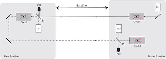
Figure 2. The MOCAST+ clock measurement scheme. CL1-3 are the clock lasers used for atom interrogation. PD1 (PD2) is a photodetector used to measure the heterodyne beat note between clock lasers to provide feedback for the laser link. BS is a (non-polarizing) beam splitter where the heterodyne beat note is formed.
Download figure:
Standard image High-resolution imageThe light beam coming from a clock laser (CL1) hosted on a Master satellite is sent towards the Slave satellite. Here, in order to regenerate the CL1 radiation, a phase lock loop with a second clock laser on the Slave satellite (CL2) is realized, similarly to what has been proposed in Hogan and Kasevich (2016). Finally, the procedure is repeated for a third clock laser (CL3) located on the Master satellite. Through appropriate timing of clocks pulses, the CL1 phase noise will affect in the same way all the three clocks, while CL3, which shares the same gravitational potential of CL1, will encode the noise due to slow baseline fluctuations.
The gravitational potential phase shift  can be thus retrieved by the double differential measurement
  where
where  is the differential phase between CL2 on the Slave satellite and CL1 on the Master satellite, and
  the differential shift between CL3 and CL1, both on the Master satellite. The expected shot noise limited sensitivity, in terms of fractional frequency, will be:

where  is the dead time between experiment cycles,
  is the atom number per clock per measurement and
  is the contrast of Ramsey fringes. Considering an optimistic scenario (interleaved operations with
  and high contrast
  ) with
  and
and  , we obtain
  , which in terms of gravitational potential corresponds to
  . It is worth to mention that, experimentally, such kind of performances on differential clock measurements have been already demonstrated on very short baselines (Bothwell et al
2022). This scheme can also work, in principle, over a much longer distance, namely hundreds of kilometres (in the optimal case about 1000 km), providing enough optical power to the clock lasers and monitoring fast position jitters with an additional optical link. Finally, it is important to remark that the repetition rate of 0.1 Hz can be enhanced by interleaving the clock interrogation on more atomic samples; this means that with an appropriate instrument engineering (i.e. several atomic sources working in parallel) also a 1 Hz regime can be achieved.
. It is worth to mention that, experimentally, such kind of performances on differential clock measurements have been already demonstrated on very short baselines (Bothwell et al
2022). This scheme can also work, in principle, over a much longer distance, namely hundreds of kilometres (in the optimal case about 1000 km), providing enough optical power to the clock lasers and monitoring fast position jitters with an additional optical link. Finally, it is important to remark that the repetition rate of 0.1 Hz can be enhanced by interleaving the clock interrogation on more atomic samples; this means that with an appropriate instrument engineering (i.e. several atomic sources working in parallel) also a 1 Hz regime can be achieved.
3. Gravity field retrieval by the space-wise approach
The space-wise approach is based on the idea of exploiting the spatial correlation of the Earth gravity field to estimate the spherical harmonic coefficients (Migliaccio et al 2004). Thereby, it is possible to obtain a solution by collocation in which the covariance of the signal is modelled as a function of the spatial distance, while the covariance of the instrumental noise is typically correlated in time. The approach gives the possibility to combine observations which are close to one another in space but distant in time, thus overcoming possible problems related to the noise temporal correlation. Nevertheless, a unique collocation procedure is not computationally feasible, mostly due to the amount of the observations to be processed. For this reason and due to the fact that a local covariance modelling is not easily achievable with a unique global covariance matrix, the space-wise approach is implemented as a multi-step procedure as shown in figure 3 (Reguzzoni and Tselfes 2009). The first step of this procedure is to estimate a set of harmonic coefficients by least squares adjustment of the potential difference observations by atomic clocks (section 3.1). This clock-only solution is later used to remove the long wavelength part of the gravity field from the gradient observations, thus reducing the signal correlation length. Nevertheless, before the reduction, the gravity gradient observations must be filtered to mitigate the impact of the instrumental noise. This filtering is performed in the frequency domain by Wiener deconvolution (section 3.2) which is followed by the gridding on a regular grid of residual gravity gradients in terms of different functionals of the gravity field, by means of a local collocation approach (section 3.3). As a final step, the gridded data are used to estimate the spherical harmonic coefficients of the gravity field by numerical integration (section 3.4) and the clock-only solution is restored.
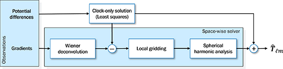
Figure 3. The space-wise approach scheme applied to MOCAST+ data processing.
Download figure:
Standard image High-resolution image3.1. Observations of potential differences and least squares solution
As a starting point, the observation equation of the potential differences, namely the observable coming from the optical clocks, can be written as:

where  is the anomalous potential,
  are the spherical coordinates of satellite
  or
or  along their orbits at a specific time
  , and
, and  is the atomic clock noise. Given the observation equation (5), we recall that the anomalous potential
  can be written in terms of spherical harmonic coefficients as

where  is the gravitational constant,
  is the mass of the Earth,
  is the reference radius of the Earth,
  is the spherical harmonic function of degree
  and order
  , and
, and  is the harmonic coefficient. The overall set of coefficients in equation (6) can be estimated by a least squares adjustment. To this aim, the deterministic model of the system can be written as

where  is the vector of the observables, namely the potential differences,
  the vector of the unknown
  spherical harmonic coefficients, and
  the design matrix where the number of rows equals the number of observations and the number of columns equals the number of unknowns, depending on the maximum spherical harmonic degree
  . The single element of matrix
  related to the observation at time
  for the coefficient of degree
  and order
  , considering the two satellites
  and
and  can be written as

Regarding the stochastic model, we considered white observation noise, with zero mean and known variance  :
:

The variance is defined according to the assumption presented in section 2. Since potential difference instead of potential is observed, the problem is ill-posed. This requires to apply a proper regularization procedure with the additional advantage of numerically stabilizing the estimates of high degree coefficients. For this purpose, either the well-known Kaula rule (Kaula 1966) or an a-prior degree variance model can be applied, introducing a regularization matrix  equal to
where  is the degree variance of the spherical harmonic coefficient
  .
.
The least-squares solution, directly estimating the spherical harmonic coefficients, is given by
where  is the regularization matrix of equation (10) and
  is the vector containing all the available observations. Then, the error covariance matrix of the estimated coefficients can be expressed as

3.2. Gradient filtering by Wiener deconvolution
Wiener filter or deconvolution (Papoulis 1981, Reguzzoni 2003, Albertella et al 2004) is a necessary step in the space-wise data processing since it is applied to reduce the time-correlated noise of the observations before the gridding. A short error correlation in time (and therefore in space) is required for gridding data on local areas, while a low error variance leads to more accurate collocation estimates. The use of either a Wiener filter or a Wiener deconvolution depends on the fact that the observations are either point-wise (as for the electrostatic gradiometers) or the outcome of an integration in time (as it happens for the quantum gradiometers based on CAI).
Based on the gradient observations proposed for MOCAST+, it is necessary to devise a deconvolution scheme accordingly. In particular, in the time domain the observation equation of the second derivatives of the gravity field is written as

where  is the vector containing the observed second derivatives (given the direction of the arm of the gradiometer),
  is the transfer function of the instrument (Migliaccio et al
2019),
is the transfer function of the instrument (Migliaccio et al
2019),  is the noiseless gravity gradient signal, the
  operator stands for the time convolution, and
  is the gradiometer measurement noise.
Starting from the analytical signal and noise ASDs presented in section 2, and also introducing the cold atom gradiometer transfer function (Migliaccio et al
2019), the Wiener deconvolution operator  can be derived by minimizing the mean square estimation error, thus obtaining

where  is the Fourier transform of the transfer function,
  is the power spectral density (PSD) of the signal
  and
and  is the PSD of the noise
  . Note that the PSD is computed as the square of the ASD. The filtered signal
  can be retrieved by applying the deconvolution operator
  to the Fourier transform of the observed second derivatives
  , together with its estimation error. The PSD of this error can be obtained as

from which the corresponding covariance function can be computed by the inverse Fourier transform. Given this covariance function, the  covariance matrix of the estimation error of the filtered signal
  can be computed and used in the collocation gridding.
The operator of equation (14) is designed by introducing the hypothesis of having a stationary process in time, with independent observation noise for instruments mounted on different satellites. Indeed, the signal observed from the different satellites is correlated, since they all fly under the action of the same gravity field. In principle this correlation may be exploited to jointly filter/deconvolve observations from all gradiometers; however, it was decided to introduce this information in the gridding procedure only, because this correlation is spatially dependent and therefore the signal covariance and cross-covariance functions are only approximately stationary in time. In other words, the Wiener deconvolution is only a pre-processing step with some approximated hypotheses, while the core of the space-wise approach is the local gridding by collocation, where the spatial signal correlation and the time noise correlation can be both properly modelled.
3.3. Local gridding by collocation
The Wiener deconvolution is followed by a collocation procedure that allows to obtain gridded data starting from the observed gravity gradients. For the proposed mission,  ,
,  , and
, and  were considered as the observed gradients, where
  is the along-orbit direction,
  is the out-of-orbital-plane direction, and
  is the radial direction. Note that if the orbit is not exactly circular, the
  direction is 'almost' along the orbit in order to maintain the
  -axis along the radial direction. The functionals to be predicted by the gridding procedure were the potential
  , the second derivative of the potential along the radial direction
  , and the second derivative of the potential with respect to the longitude
  . Note that the last quantity is not formally a gravity gradient because it is a second derivative with respect to an angle and has the same measurement unit of the potential
  . As a starting point, the observation equation corresponding to the position at epoch
  is written as

where  are the coordinates at time
  , the vector
  contains the Wiener filtered gradients, and
  is the estimation error of the Wiener deconvolution, see equations (14) and (15).
The gridding procedure is done by collocation over local patches of data, since a global collocation procedure would be numerically unfeasible (Migliaccio et al 2006, Reguzzoni et al 2014). Moreover, with local collocation it is possible to avoid numerical drawbacks due either to considering a too large amount of data at once, or to including observation points which are too close to each other. The estimated grid is defined on a spherical boundary at a constant altitude equal to the mean satellite altitude (or at least included between the lower and higher orbit altitudes, in case of many satellites), and each grid node is computed by considering the neighbouring data. Therefore, one of the most crucial parts of the gridding procedure is the determination of the local patches of data based on the position of the nodes. To enhance the local information, more observations are used in the proximity of the grid node to be estimated, also applying the condition that the same set of points must not be used to estimate different grid nodes.
The partitioning of the set of data points to be considered for the estimation of grid nodes is done by dividing the point patch into three areas with different size and point density. The size of the patch depends on the correlation length of the covariance function of the data, while the size of each area varies depending on the amount of the available data points, implying a possible data under-sampling. A representation of this 'adaptable' patch of data points can be seen in figure 4.

Figure 4. Example of a patch of points (blue dots) used as input for the gridding procedure (angular distance measured in degrees); the three areas with different spatial densities are bounded by dashed green lines, while red crosses represent the grid nodes to be estimated by using the point patch.
Download figure:
Standard image High-resolution imageBefore proceeding with the collocation step, the long-wavelength effects must be removed from equation (16), so the clock-only solution computed by equation (11) is subtracted from the original observation equation, obtaining

where  represents the gravity signal computed by the synthesis of the
  spherical harmonic coefficients estimated by the least squares solution of equation (11). Recalling both equation (16) and the following formula

where  is the error of the gradients synthesised from the clock-only solution, namely the missing signal to be retrieved by the gridding procedure, the observation equation can be written as

From here, the collocation estimate can be derived as

where  is the functional of the gravitational field (i.e.
  ,
,  , or
, or  ) to be estimated at the grid node with coordinates
  starting from the given set of observations
  ,
,  is the covariance matrix of the observed functionals in the neighbourhood of the grid node,
  is the cross-covariance matrix between the observed functional and the one to be estimated, and
  is the covariance matrix of the Wiener deconvolution estimation error. Note that
  and
and  can be computed from equation (12) and locally adapted based on the data inside each point patch, while
  is computed according to equation (15). Also note that, whereas the signal
  (and therefore
  ) is uncorrelated from the gradiometer noise
  , the Wiener deconvolution introduces a correlation between the signal and the estimation error
  . This correlation can be properly considered by iterating the general scheme of the space-wise approach (Reguzzoni and Tselfes 2009), but here it has been neglected to speed up the computations, given the need of performing a large number of simulations. This approximation is expected to mainly affect the estimation of the highest spherical harmonic degrees.
3.4. Spherical harmonic analysis
Considering the observation equations (16) and (19) and rewriting them for the estimated grid values, we obtain

where  is the estimated functional (i.e.
  ,
,  , or
, or  ) and
) and  is the gridding error. The gridding procedure to compute each of the estimated functional directly includes the combination of the observations from all satellites, meaning that all the observed gradients falling inside one patch are directly combined through equation (20) to estimate grids of
  ,
,  , or
, or  values.
For each of the grids, the spherical harmonic coefficients are derived by numerical integration, computed over the spherical boundary, based on quadrature equations (Colombo 1981)

where the indexes  and
and  are used to identify the grid nodes,
  is the size of the equiangular grid cell around each the grid node
  , and
, and  is the (transfer) function that depends on the type of
  functional, which is equal to


The spherical harmonic coefficients computed from the three estimated grids are then combined to obtain a unique solution. This combination can be performed by weighting the coefficients from different grids according to their estimation errors computed by a Monte Carlo approach (Migliaccio et al
2009). According to this approach, the kth sample of the spherical harmonic coefficients  was drawn from a reference global gravity model (considering its error degree variances) and used to simulate observations along the orbit together with a random sample of the instrumental noise. Then, the simulated observations entered the space-wise computation scheme (figure 3) and grid values
  with the corresponding coefficients
  were estimated for each sample
  , so that the empirical error rms can be computed as
where  represents the overall number of Monte Carlo samples. The coefficient variances computed by equation (26) were used to determine the combination of the spherical harmonic coefficients coming from grids of different functionals as:
Given this combination for each of the  samples, the empirical error rms of the resulting spherical harmonic coefficients can be computed as
Note that the combination in equation (27) is not optimal because covariances and cross-covariances are neglected due to the fact that their computation would require a very high number of Monte Carlo samples.
As for the grids, the error rms at each node can be similarly computed as
4. Numerical simulations
A series of different datasets were generated for simulation purposes. As reference model, EGM2008 (Pavlis et al
2012) was used for the generation of the signal Monte Carlo samples, consistently with the model used in the orbit simulations. The orbit dataset is composed of two orbits with a pair of satellites along each orbit, i.e. a polar orbit ( 89°) and an inclined orbit (
 66°), with mean altitudes equal to 371 km and 347 km, respectively. The orbital dataset was characterized by a 20 s sampling rate over a complete simulation of about 118 days and it was then interpolated at a 1 s sampling rate for time spans equal to about one month, two months, and four months by means of Lagrange polynomials.
For the non-tidal mass variations in the atmosphere, ocean, hydrology, ice, and solid Earth (AOHIS) and for de-aliasing purposes, the updated ESA Earth system model (ESM) was used (Dobslaw et al 2015, 2016). This model allows to simulate the effects of the non-tidal temporal variations of the gravity signal on monthly gravity field solutions. This model is not randomly sampled and therefore the simulated time-variable signal is the same for all the Monte Carlo samples.
During the study, several mission scenarios were considered based on the values of the parameters that have the highest impact on the observations, such as
- satellite mean altitude,
- inter-satellite distance,
- satellite formation (GRACE-class formation on polar orbit or Bender-class formation),
- number of in-line satellites on the same orbit (two or three),
- clock observation sampling rate (0.1 or 1.0 Hz),
- noise PSDs of the gradiometers (figure 1), depending on the atomic species used in the CAI (Rb or Sr) and on the accuracy of the attitude control sensors (no control, 1 nrad s−1, full control),
- orientation of the gradiometer arm along different directions (
 , , or ) on different satellites (always considering one gradiometer per satellite).


The first simulations that were performed focused on the impact of the atomic clock observations, so a series of least squares clock-only solutions were computed by changing the values of the first five parameters of the above list. Later, these solutions were used to remove the long-wavelength part of the gravity field, introducing the gradiometer observations in the gridding procedure and exploiting the full space-wise solution as presented in section 3. The impact of introducing gradiometer data in the gravity field estimation was studied by considering different gradiometer noise PSDs and different orientations of the gradiometer arm, i.e. considering the last two parameters of the above list. Finally, the impact of adding the time-variable component of the gravity field to the simulations was investigated for the mission configurations providing the best results with the static gravity field only.
The number of simulated Monte Carlo samples was equal to 100, guaranteeing a good convergency of the error estimates without increasing too much the computational burden.
4.1. Clock-only simulations and results
For the clock only simulations, three main satellite orbit configurations were considered. They consist of a GRACE-class formation with a pair of satellites on a polar orbit, a Bender-class formation with two pairs of satellites on polar and inclined orbits, and finally a Bender-class formation with three satellites along each orbit.
Each one of these formations was tested for different sampling rates, different inter-satellite distances and, only in the case of the GRACE-class formation, for different satellite altitudes. As for the last point, increasing or lowering the satellite orbit altitude by 120 km with respect to the nominal one shows that the lower orbit scenario, as expected, can provide an improvement at medium-high harmonic degrees (see yellow line in figure 5), while increasing it would have a significant negative effect on the quality of the estimation (see blue line in figure 5). However, lowering the altitude has a limited impact on the low harmonic degrees (the most important ones for time-variable gravity field analysis) and would shorten the mission lifetime. Therefore, this parameter was neglected in the subsequent simulations.

Figure 5. Error degree variances of clock-only solutions testing different orbital altitudes considering a pair of satellites on a polar orbit, with 100 km inter-satellite distance and 0.1 Hz clock sampling rate.
Download figure:
Standard image High-resolution imageScenarios based on a Bender-class formation allow to improve the results with respect to the GRACE-class formation. Some significant results are reported in figure 6, showing the accuracy of different simulations in terms of error degree variances, computed according to equation (28). Note that the Monte Carlo empirical error variances are basically equivalent to the formal error variances taken from the diagonal of the covariance matrix in equation (12). Considering the Bender-class formation with two satellites per orbit, the quality of the estimated solution can be improved by about two orders of magnitude (in terms of variance) by increasing the inter-satellite distance from 100 km to 1000 km (according to the theoretical limits for this technology, as described in section 2), as it can be seen by comparing the blue and yellow lines in figure 6. Moreover, if the clock observation sampling rate is increased from 0.1 Hz to 1 Hz, this leads to an improvement of about one order of magnitude, as it can be seen by comparing the solid and dashed lines in figure 6. Finally, simulations with an additional third satellite on both the polar and the inclined orbit were performed, in order to increase the spatial resolution and the number of observations. In this case the inter-satellite distance between pairs of satellites was set equal to 1000 km, allowing to slightly improve the results of the previous configurations, as it can be seen in figure 6 by comparing the purple line with the other ones. The three cases presented in figure 6 represent the best-case scenarios for the clock-only solutions, and they are compared with the error degree variances from GRACE. The latter were obtained by the monthly average of ITSG-GRACE 2018 errors (Kvas et al 2019) over a time span of about 14 years. As it can be seen, unfortunately the usage of atomic clocks only is not sufficient to ensure a gravity field solution better than the GRACE one. Only the Bender configuration with six satellites and a clock observation frequency of 1 Hz (dashed purple line in figure 6) could approach the GRACE error level, improving a few very low harmonic degrees.

Figure 6. Error degree variances of clock-only solutions for selected simulations with Bender configuration: two satellites per orbit with an inter-satellite distance  of 100 km (blue lines) or 1000 km (yellow lines) and three satellites per orbit with inter-satellite distance
  of 1000 km (purple lines). Solid and dashed lines represent solutions for 0.1 Hz and 1.0 Hz clock observation frequency, respectively.
Download figure:
Standard image High-resolution image4.2. Clock and gradiometer simulations and results
Coming to the main part of the payload, which is the CAI, the simulations were aimed at investigating the impact of the gradiometer arm orientation, which is related to the orbital inclination (polar or inclined) as well as to the different noise PSDs (in turn depending on the level of accuracy which could be achieved with the attitude compensation of the atmospheric drag and other torques, see again figure 1). For this purpose, a period of one month was considered for each simulation; no other gravitational or non-gravitational effects (tidal and non-tidal mass variations) were taken into account.
Before presenting the results of the simulations, it is important to stress the impact of the accuracy of the attitude control sensor on the gravity gradient measurement in the orbital plane (thus involving gradiometers mounted in the along-track  -axis and in the radial
  -axis directions). In fact, angular rotations, through the centrifugal term, put a serious limitation to these measurements. For this reason, compensation of the residual angular rotations around the out-of-orbital-plane
  -axis direction is needed; the accuracy of this compensation highly influences the gradiometer accuracy on the along-track
  -axis and radial direction
  -axis, as already shown in section 2. To understand the impact of changing the gradiometer arm direction (
 ,
,  ,
,  ), the solutions of a series of scenarios considering observations from a single gradiometer mounted onboard a single satellite (along the polar or inclined orbit) were computed, introducing all possible combinations between gradiometer arm direction and drag compensation level. To allow for a proper comparison, the same long-wavelength model of the gravity field was removed before the gridding procedure for each simulation. For this purpose, the clock-only solution for the Bender-class formation with two pairs of satellites at 100 km inter-satellite distance and 0.1 Hz clock sampling rate (solid blue line in figure 6) was used.
The results for the polar and inclined orbits are shown in figures 7 and 8, respectively. The best solution was obtained by orienting the gradiometer arm along the radial direction ( -axis), considering the scenario with a full attitude compensation level. As already discussed in section 2, this is an ideal scenario, therefore the best solution is actually obtained by orienting the gradiometer arm along the out-of-orbital-plane direction (
 -axis), since in this case the instrumental accuracy is not affected by the accuracy of the attitude control. Note that the inclined orbit is affected by quality degradation due to the data gaps at high latitudes, which lead to a solution degradation between degrees 20 and 120, where the error degree variances are dominated by the higher error of the lower order coefficients. For this reason, to better evaluate the accuracy achievable by exploiting different gradiometer directions, the degree variances were replaced by the squared degree medians of the coefficient error, which are shown in figure 8(b).
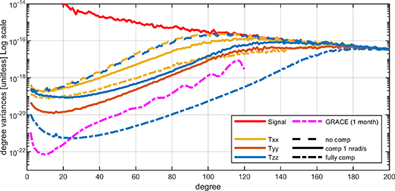
Figure 7. Error degree variances considering a single-satellite single-gradiometer scenario on polar orbit for different orientations of the gradiometer axis. Colours represent the gradiometer arm direction; line styles represent the accuracy of the attitude control, as shown in the legend. The three error curves for the  gradiometer are overlapping, since this direction is not affected by degradation in the attitude control.
Download figure:
Standard image High-resolution image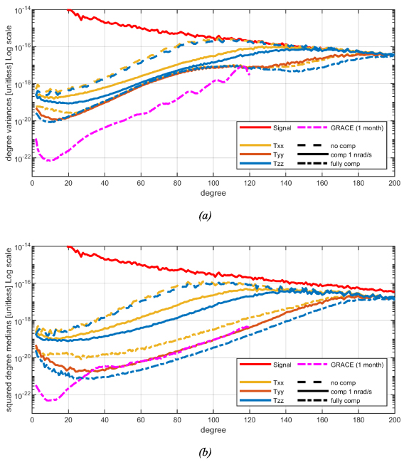
Figure 8. Error degree variances (a) and squared degree medians (b) considering a single-satellite single-gradiometer scenario on inclined orbit for different orientations of the gradiometer axis. Colours represent the gradiometer arm direction, line styles represent the accuracy of the attitude control, as shown in the legend. The three error curves for the  gradiometer are overlapping, since this direction is not affected by degradation in the attitude control.
Download figure:
Standard image High-resolution imageA further comparison of the impact of different gradiometer axis orientations was performed at the level of the single spherical harmonic coefficient, considering only the most realistic case with 1 nrad s−1 attitude control accuracy. The results of this comparison are shown in figure 9. Here, the gradiometer arm direction providing the best estimate, i.e. providing the smallest error variance, is shown for each harmonic degree and order. With this level of attitude control accuracy, the main contribution to the coefficient estimation comes from the gradiometer oriented along the  -axis direction, as it can also be observed from figures 7 and 8. This finding is in agreement with previous works on quantum gradiometry, see e.g. Douch et al (2018). Nevertheless, a contribution coming from
  at low orders can be seen on the polar orbit. As for the inclined orbit this contribution is still present, but extremely limited if compared to
  .
.

Figure 9. Comparison between error variances of spherical harmonic coefficients estimated by observing the gravity gradients in different directions (x, y, z), considering attitude control at the level of 1 nrad s−1; the gradients leading to the smallest error variance are shown for each degree and order.
Download figure:
Standard image High-resolution imageThe altitude at which gridded data are predicted is another parameter to be considered in the possible combinations. To check its impact, the following values of the grid altitude were tested: 347 km (mean altitude of the inclined orbit), 371 km (mean altitude of the polar orbit), and 360 km (overall average altitude of the two orbits). However, the results (computed for a single gradiometer on a single satellite) showed a negligible impact of the choice of altitude, therefore in the following simulations the grids were always computed at the average altitude of 360 km.
Given the results of the single-satellite gradiometer simulations, the analysis focused on Bender-class formations with pairs or triplets of in-line satellites, always setting the inter-satellite distance at about 1000 km, thus considering only the best conditions for the clock-only solutions, according to the results presented in figure 6. The comparisons were performed between the best ideal scenario (full attitude compensation) and the more realistic one (1 nrad s−1 attitude compensation). In the last scenario, gradiometers with different atomic species were considered too. Under these conditions, three mission configurations were simulated based on Bender-class formations with two or three satellites per orbit:
- ideal, with full attitude compensation, mounting gradiometers on all satellites;
- realistic with Sr gradiometer, with 1 nrad s−1 attitude compensation, mounting gradiometers on all satellites apart from a single gradiometer on the polar orbit;
- realistic with Rb gradiometer, with 1 nrad s−1 attitude compensation, mounting gradiometers on all satellites apart from a single gradiometer on the polar orbit.


The gradiometer arm directions were chosen based on the error curves presented in figures 7 and 8, while the choice of mounting a  gradiometer on a satellite along the polar orbit for realistic scenarios was driven by the results presented in figure 9. A further scenario was devised for the three-satellites-per-orbit configuration, based on one
  gradiometer on board the central satellite of each orbit, in order to minimize the complexity and cost of the mission. It seems reasonable to assume that the central satellite plays the role of master with the gradiometer and two tracking clock systems pointing towards the other two satellites; anyway, the choice of the master does not affect the results of the analysis. The least squares clock-only solution needed to reduce the long-wavelength required by the gridding procedure was computed according to the satellite configuration of each scenario, always considering 1 Hz atomic clock sampling rate.
The results of these simulations are shown in figure 10 (Bender, two satellites per orbit) and figure 11 (Bender, three satellites per orbit), where the empirical error degree variances from Monte Carlo simulations are also compared with the error degree variances from GRACE.

Figure 10. Clock and gradiometer joint solutions for the tested scenarios in the case of a Bender configuration with two satellites per orbit and an inter-satellite distance  of about 1000 km. Solid blue line represents the clock-only solution used to compute the combined solution; dashed magenta line represents the GRACE accuracy for comparison purposes.
Download figure:
Standard image High-resolution image
Figure 11. Clock and gradiometer joint solutions for the tested scenarios in the case of a Bender configuration with three satellites per orbit and an inter-satellite distance  of about 1000 km. Solid blue line represents the clock-only solution used to compute the combined solution; dashed magenta line represents the GRACE accuracy for comparison purposes.
Download figure:
Standard image High-resolution imageThe error curves of figures 10 and 11 show that the Bender-class formation with two or three satellites per orbit allows to estimate spherical harmonic coefficients up to about degree 200 with only one month of observations, irrespectively of the chosen mission configuration. This is quite a remarkable result, when compared with GRACE and GOCE performances. Note that the best solution was obtained when using ideal conditions with a full attitude control (see red line in figures 10 and 11) and represents a sort of theoretical limit for this kind of instruments and orbit configurations. As for the impact of using Sr instead of Rb as atomic species, an improvement by a factor ∼2 in terms of standard deviation was obtained above degree 20, as shown by the comparison of the yellow and purple lines in figures 10 and 11. This improvement is mainly due to the lower level of the Sr gradiometer noise PSD (see figure 1), while the lower degrees are also controlled by the clock-only solution, which is the same for the two scenarios. The configuration with only two  Sr gradiometers shows an error which, below degree 100, is of the same level of the one with six Rb gradiometers, confirming the possibility of reducing costs and mission complexity without losing too much in terms of accuracy.
A further test was performed to assess the impact of the clocks on the computed solutions. To this aim, the realistic configuration with six satellites (attitude control at 1 nrad s−1 level with five  and one
 gradiometers) was considered introducing a degraded accuracy in the potential difference observations (by a factor 10 in terms of noise variance). Note that the same degradation can be obtained by working at 0.1 Hz with the nominal clock accuracy. The result of this degraded scenario is compared with the one previously computed with the same satellite configuration and the nominal clock accuracy of 0.2
  (see figure 12). The differences between the two solutions are in the lower degrees, namely below 50, where better measurements from clocks can improve the quality of the overall solution up to one order of magnitude (compare the red and blue solid lines in figure 12). However, the clock-only solution never 'dominates' the error curve at low degrees. Therefore, the improvement could be partially related to the role of the clock-only solution in the space-wise approach, particularly in the data reduction before the gridding affecting the signal covariance modelling (see equations (17)–(20)).
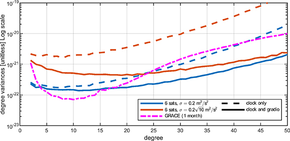
Figure 12. Error curves for the Bender scenario with six satellites (attitude control at 1 nrad s−1 level with five  and one
 gradiometers) considering different accuracies of the clock observations (represented by different colours). Dashed lines represent errors of the clock-only solutions; solid lines represent the error of the joint clock and gravity gradient solutions.
Download figure:
Standard image High-resolution imageFor the sake of completeness, the cumulative commission errors for geoid undulations and gravity anomalies at ground level (in spherical approximation) were computed and are shown in figures 13 and 14 for the ideal scenario ( on all the satellites with a full attitude control) and for the realistic scenario (
 on all satellites apart from the one with
  considering a 1 nrad s−1 attitude control), either in the case of two or three satellites per orbit in Bender-class formation.

Figure 13. Cumulative commission error in terms of geoid undulations, considering ideal and realistic case simulations for Bender configurations with two or three satellites per orbit, ∼1000 km inter-satellite distance and 1 Hz clock observations.
Download figure:
Standard image High-resolution image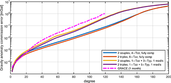
Figure 14. Cumulative commission error in terms of gravity anomalies, considering ideal and realistic case simulations for Bender configurations with two or three satellites per orbit, ∼1000 km inter-satellite distance and 1 Hz clock observations.
Download figure:
Standard image High-resolution imageFinally, the impact of longer time span solutions was tested for the Bender-class formation in the nominal mission case (one pair of satellites along each orbit at 100 km inter-satellite distance). The error grids of the different time span solutions, computed as the standard deviation of grid errors over 100 Monte Carlo samples, are shown in figure 15 in the case of the second radial derivative  . As it can be seen, increasing the period covered by the solution leads to a more uniform precision, thanks to the denser data distribution. In fact, the one month and two months gravity field solutions still show a visible pattern coming from the orbit ground tracks, while this pattern is strongly reduced in the four-month solution. Additionally, figure 15(d) shows the root mean square error for each point of the grid (for the four-month solution only), thus also showing systematic effects that are not correctly retrieved in the solution and, therefore, are present in all Monte Carlo samples. As expected, some high frequencies are not estimated, mainly depending on the satellite altitude and gradiometer accuracy, as well as on the processing strategy, which was not optimized for the estimation of such high-degree coefficients (i.e. too large clouds of data).

Figure 15.
 grid estimation error in terms of standard deviation, for different solution periods: (a) one month; (b) two months; (c) four months; in the lower right panel (d) the root mean square error for the four-month scenario is also represented, to highlight the systematic effects that are not correctly retrieved due to limited spectral resolution.
Download figure:
Standard image High-resolution image4.3. Impact of the time-variable component on the simulation results
The MOCAST+ study was completed by investigating the effects of the non-tidal mass variation on the gravity field generated by the variability in atmosphere (A component), oceans (O component), continental ice-sheets (I component), groundwater (H component), and solid Earth (S component) on the estimation accuracy of monthly solutions, considering different mission scenarios. One of the main problems caused by the time-variable component is the presence of aliasing in the computed solution. The aliasing effect is related to the gravity signal with frequency higher than one month (e.g. from hours to days in atmosphere, oceans, and, considering smaller spatial extent, also in groundwater) and background model errors of these signals. The magnitude of this aliasing effect is usually higher than the noise level of the instruments, which are the CAI for the proposed MOCAST+ mission or the K-band ranging system for GRACE and GRACE-FO missions (Wiese 2011, Wiese et al 2012).
For the purposes of this investigation, three mission configurations were tested, namely:
- a GRACE-class formation, with pair of satellites on a polar orbit, with one gradiometer and one gradiometer;
- a Bender-class formation with a pair of satellites per orbit, with one gradiometer on the polar orbit and three gradiometers on the inclined orbit;
- a Bender-class formation with a triplet of satellites per orbit, with one gradiometer on the polar orbit and five gradiometers on the inclined orbit.


In all cases the clocks were assumed to work at 1.0 Hz sampling rate and the attitude control was assumed to have a 1 nrad s−1 accuracy. For all simulations only non-tidal mass variations were considered by introducing the ESA updated ESM (Dobslaw et al 2015). In particular, the overall effect due to AOHIS was added to the static gravity field of each Monte Carlo sample and reduced with the de-aliasing model (DEAL) provided with the updated ESM. To properly account for model errors in the AO components of DEAL, this term was corrected by the AOerr model (also provided with the updated ESM), thus allowing to simulate a realistic scenario with a consistent dataset (Dobslaw et al 2016).
For the simulations, the signal of January 2001 was considered in all Monte Carlo samples. The chosen realization of the monthly average of the residual time variable signal (computed as AOHIS–DEAL–AOerr) is shown in figure 16 in terms of both potential and second radial derivative computed at the satellite mean altitude of 360 km.

Figure 16. Monthly average of the residual time variable signal (computed as AOHIS–DEAL–AOerr) at the mean satellite altitude of 360 km, in terms of potential and second radial derivative.
Download figure:
Standard image High-resolution imageThe results obtained in the three simulated scenarios are presented in figures 17 and 18 showing the empirical error degree variance curves for the clock-only and the clock-gradiometer solutions, respectively. Here, the estimation error is compared with the error obtained for the static gravity field only (i.e. following the same simulation scheme used in section 4.2). In order to compute the empirical errors when the signal includes non-tidal temporal variations, the estimates obtained for each Monte Carlo sample are compared with the corresponding reference static model plus the monthly average of the time-variable signal.

Figure 17. Error degree variances of the three simulated scenarios, introducing the effect of the time-variable (TV) component of the gravity field in the clock-only solution. Solid lines represent the error when this component is introduced in the simulation; dotted lines represent the error without this component, i.e. the best obtainable solution given the specific mission configuration; purple solid line represents the power of the TV component.
Download figure:
Standard image High-resolution image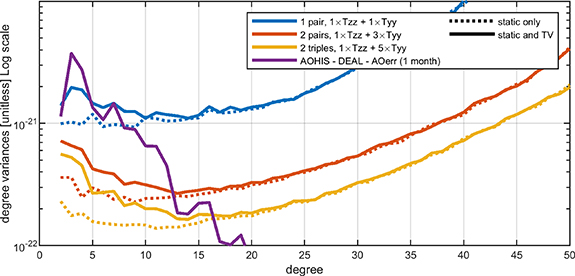
Figure 18. Error degree variances of the three simulated scenarios, introducing the effect of the time-variable (TV) component of the gravity field in the clock and gradiometer solution. Solid lines represent the error when this component is introduced in the simulation; dotted lines represent the error without this component, i.e. the best obtainable solution given the specific mission configuration; purple solid line represents the power of the TV component.
Download figure:
Standard image High-resolution image
The error curves show that there is a degradation in the quality of the solution below degree 20 due to the presence of non-tidal mass variations (compare the solid and dotted lines in figures 17 and 18). As expected, the Bender-class formation significantly improves the capability of detecting the time variable gravity signal with respect to the GRACE-class formation. This is true in the clock-only solution, but especially in the clock-gradiometer joint solution. The transition from two to three in-line satellites per orbit is not really effective in improving the quality of the clock-only solution, while it has a significant impact on the clock-gradiometer joint solution (compare the red and yellow solid lines in figures 17 and 18, respectively). This may be due to the role of the gravity gradients in the solution, but also to the data gridding procedure that is able to locally average the time-variable signal mitigating its impact at a global level.
All the solutions which included non-tidal mass variations were computed by applying the same parameter calibration used in the solutions for the static gravity field (e.g. regularization in the least squares solution, local adapting of covariance function in the gridding procedure, etc, see section 3). Therefore, it can be concluded that part of the error increment shown in figure 18 is related to the space-wise algorithm, which should require a finer tuning to better exploit the time-variable information included in the data.
5. Discussion and conclusions
The paper presented the proposal of a possible future gravity mission based on quantum technology exploiting the idea of the satellite-to-satellite tracking along the same orbit, like GRACE, but using an optical link between atomic clocks. In this way, the observed quantity is not the range (or range variation) between two satellites, but the time difference which can be straightforwardly related to the gravitational potential difference. Each satellite is also equipped with a quantum gradiometer, exploiting the CAI, thus realizing a sort of joint GRACE-GOCE mission principle. Furthermore, instead of considering a GRACE-class formation with a pair of satellites on a single orbit, also a Bender-class formation with both a polar and an inclined orbit was tested, thus including in the proposal the concept of a satellite formation which is under study for the future NGGM/MAGIC mission. Furthermore, in the framework of the Bender-class formation, a more complex (and also expensive) solution based on three in-line satellites per orbit was assessed to quantify the possible improvements. So, a large spectrum of mission scenarios was considered, with the main target of investigating whether the joint use of atomic clocks and quantum gradiometers could significantly improve the current knowledge of the gravity field. In particular, the results were compared with GRACE error level, since GRACE is the mission currently providing the best information at low spherical harmonic degrees, which are useful for the investigation of time-variable phenomena.
Data from numerical simulations were analysed by exploiting the space-wise approach, which for this study was simplified (e.g. with respect to the GOCE data processing scheme) to have the possibility of analysing many scenarios within a reasonable computational time. According to this technique, potential differences from atomic clock observations are processed by least-squares adjustment (assuming white noise), while gravity gradients from CAIs are filtered and then mapped on a spherical grid by using the collocation method. The result is represented by a set of spherical harmonic coefficients and error estimates based on Monte Carlo samples.
The findings of the study are summarized in the following points.
- Clock-only solutions, i.e. without any gradiometer on board the satellites, are generally weaker than GRACE solutions for corresponding time-spans (one month in our simulations). This result is obtained even assuming quite optimistic performances of the atomic clocks and a very long baseline of about 1000 km between satellites. Only the Bender configuration with six satellites and 1 Hz clock observations could emulate the GRACE performances, actually slightly improving the estimation of the very low spherical harmonic degrees. However, such inter-satellite distance and sampling rate would imply increasing the technological complexity of the mission.
- Clocks seem to be anyway useful for the processing of the gravity gradients in the framework of the space-wise approach. In fact, it was seen that the better is the clock solution, the better is the gravity gradient reduction and, consequently, the estimation of the spherical harmonic coefficients especially at low degrees. In other words, even if the clock-only solutions are not very competitive with GRACE solutions, they are able to provide information that couples quite well with the one provided by the gravity gradients.
- A single arm gradiometer is proposed, and it is quite clear that the optimal axis of this arm is along the out-of-orbital-plane direction to avoid the degradation implied by the limited spacecraft attitude control (assuming 1 nrad s−1 accuracy). Actually, considering the polar orbit, the radial axis can provide useful information for the estimation of the low order spherical harmonic coefficients, even considering the above-mentioned attitude compensation problem. For this reason, it is recommended to use only gradiometers along the out-of-orbital-plane direction, apart from one oriented in the radial direction to be mounted on board one of satellites flying in the polar orbit.
- Gravity gradients from quantum technology, exploiting the flat noise PSD at low frequency (differently from the electrostatic gradiometers, see figure 1), contribute to the coefficients estimate also at low degrees. The clock-gradiometer joint solution, for a Bender configuration with three satellites per orbit, shows better performances than GRACE above harmonic degree 15 (the geoid undulation commission error is about 1 cm up to degree 100, against the 2–3 cm of GRACE). With one month of observations, the maximum harmonic degree is 200 for the Bender formation with two or three satellites per orbit, which is better than GRACE and GOCE results.
- Aliasing effects due to the time variable component of the gravity signal, as it is already known, are reduced by subtracting a de-aliasing model from the data and by selecting a Bender-class formation, with a further improvement obtained by adding the third satellite on each orbit. From the numerical simulation results, it was seen that using gradients as observations and processing them by local gridding can provide a quite significant impact on the solution accuracy.
Acknowledgments
We acknowledge the contribution of the partners of the MOCAST+ ASI funded project: Carla Braitenberg(1), Guglielmo Maria Tino(2), Fiodor Sorrentino(3), Sergio Mottini(4), Khulan Batsukh(5), Tommaso Pivetta(1), Alberto Pastorutti(1), Simona Zoffoli(6) of the following institutions: (1) University of Trieste, Department of Mathematics and Geosciences, Trieste, Italy; (2) University of Florence, Department of Physics and Astronomy, Florence, and LENS Laboratory, Florence, Italy; (3) The National Institute for Nuclear Physics, Genova, Italy; (4) Thales Alenia Space Italia, Turin, Italy; (5) Politecnico di Milano; (6) Italian Space Agency (ASI), Rome, Italy.
Data availability statement
The data generated and/or analysed during the current study are not publicly available for legal/ethical reasons but are available from the corresponding author on reasonable request.
Conflict of interest
The authors have no relevant financial or non-financial interests to disclose.
The authors have no competing interests to declare that are relevant to the content of this article.
Funding
The study presented in this paper was funded by the Italian Space Agency ASI (Agenzia Spaziale Italiana) under ASI Contract No. 2019–16-U.0 'MOCAST+ MOnitoring mass variations by Cold Atom Sensors and Time measures'.