
Abstract
The motion of trapped atoms plays an essential role in quantum mechanical sensing, simulations and computing. Small disturbances of atomic vibrations are still challenging to be sensitively detected. It requires a reliable coupling between individual phonons and internal electronic levels that light can readout. As available information in a few electronic levels about the phonons is limited, the coupling needs to be sequentially repeated to further harvest the remaining information. We analyze such phonon measurements on the simplest example of the force and heating sensing using motional Fock states. We prove that two sequential measurements are sufficient to reach sensitivity to force and heating for realistic Fock states and saturate the quantum Fisher information for a small amount of force or heating. It is achieved by the conventionally available Jaynes–Cummings coupling. The achieved sensitivities are found to be better than those obtained from classical states. Further enhancements are expectable when the higher Fock state generation is improved. The result opens additional applications of sequential phonon measurements of atomic motion. This measurement scheme can also be directly applied to other bosonic systems including cavity QED and circuit QED.
Export citation and abstract BibTeX RIS

Original content from this work may be used under the terms of the Creative Commons Attribution 4.0 licence. Any further distribution of this work must maintain attribution to the author(s) and the title of the work, journal citation and DOI.
1. Introduction
The interaction between bosons and a two-level system establishes the basic fundamentals of quantum theory and leads to various applications and developments of advanced technologies. However, for some physical systems, including trapped ions, cavity QED and circuit QED, the bosonic state cannot be directly accessible but can only be inferred through the detection of the two-level system [1–4]. The direct readout is especially challenging for trapped ions as phonons cannot propagate out of the system. Additionally, electrodynamically trapped and optically cooled ions already proved to be ideal objects for tests and applications of quantum mechanics [1, 5–7]. Quantum motion of trapped atoms is a subject of interest for quantum sensing of mechanical and electric atomic effects [8, 9], quantum simulations of diverse phenomena [10, 11], development of quantum computing platforms [12, 13], but also the developing field of quantum thermodynamics [14, 15]. Highly sensitive phonon measurements are pivotal here, although such measurements can have limited dynamic ranges. It is reminiscent of a situation in photon counting [16–18], in which single-photon detectors allowed a new regime of high sensitivity. Their multiplexing using a reliable beam splitter coupling gave rise to further developments of powerful detection techniques for light despite their limited photon number resolution [16]. Their response in terms of photo-click statistics gives sufficient information to either estimate photon number distribution or to directly detect fundamental features of light [16, 19]. These approaches can consider and optimize the beam splitter couplings to reach the smallest error. For trapped atoms, phonons can only be detected through discrete internal levels of the atom coupled to an optical transition [20]. The most conventional and straightforward detection of phonons in trapped, cooled ions is based on optical detection of Rabi oscillations between electronic levels [13]. Conventionality is crucial here as we expect our proposed detection to be successfully achieved by commonly used technologies.
In principle, repeating the conventional detection can give more extensive information about the phononic occupation, although it does not give the exact phonon resolution. The simplest example is the detection of classical mechanical force and heating of atoms. From previous studies, mechanical heating can be sensed under the assumption that the motional state is in a thermal state, while its mean phonon number is extracted through a spin population measurement [1, 21–23]. On the other hand, there are several approaches that have been proposed to sense mechanical force [24–26], for example using motional non-Gaussian compass states as a probe [26]. Recently, mechanical Fock states of n phonons have been demonstrated to give an improved sensitivity using a binary projection on that phonon number n [8]. Here, to illustrate the applicability of the proposed sequential measurement, we apply it to sense force and heating of trapped ions. We compare the sensitivity for a finite sample to both the quantum Fisher information upper bound and the projection on the phonon number. We predict that two optimized steps of detections based on very reliable Jaynes–Cummings interaction are already sufficient for both of the sensing tasks with currently realistic Fock states and damped Rabi oscillations in the process. Particularly, we address photon recoil limitation in the trapped ion measurements. It opens a direct path to experimental verification and stimulates further theoretical proposals based on this sequential phonon measurement. It can be extended into a toolbox for the direction of phonons in the same way as the multiplexed single-photon detection a decade ago.
2. Sequential measurement
Let us first describe a sequential qubit readout of the motional state of trapped ions. The internal electronic-level qubit, detectable optically, is employed to monitor the change of the motional state, as a direct optical measurement of the motional state with high efficiency is technically difficult. A sequential interaction of the qubit with the motional state is the simplest extension to reach sufficient sensitivity. The two-step indirect measurements of the motional state are summarized in the quantum circuit portrayed in figure 1(a).

Figure 1. (a) The quantum circuit for two sequential measurements of the motional state ρmo. The most basic Jaynes–Cummings interactions between the internal qubit and motional state of trapped ions are described by two unitary operators  JC, each followed by a measurement on the internal state. The second interaction time,
  or
or  , is chosen based on the outcome of the first measurement. (b) For trapped ions, the second measurement is performed only when the outcome of the first measurement is found in a dark state and ceased otherwise to avoid the photon recoil effect. The interactions between the internal qubit (red) and mechanical oscillator (blue) are used for the scheme of quantum sensing with the sequential measurements. The first measurement found in a dark state causes the total state of the system, both the qubit and the mechanical state, collapse into a particular state. The second interaction, therefore, has to be tuned in accordance with the first result:
  if it is in the dark, excited (ground) state.
Download figure:
Standard image High-resolution imageTo couple the internal and motional states, an electromagnetic field with its frequency tuned to the red sideband is applied to the ions. In the Lamb–Dicke regime of small motional excitations, this reliably gives rise to the Jaynes–Cummings interaction with the Hamiltonian in the interaction picture written as

where λ is the coupling strength, and φ is an initial phase of the electromagnetic field. For simplicity, we set φ = 0. It is the most used and controllable interaction broadly accessible for many trapped-ion experiments [1, 13]. The time evolution of the internal and motional states, after interacting for a time t1, is described by the unitary transformation, UJC
 , depicted as the first unitary gate UJC(t1) in figure 1(a). After that, a measurement on the internal state in the internal-state basis
  is performed. We note here that, instead of using the red-sideband interaction, one can alternatively use the blue-sideband, described by anti-Janes–Cummings Hamiltonian [1, 20]. In this case, all calculations in this work can still be used by replacing the notation of the internal excited state
  with that of the ground state
  and vice versa.
Due to the small dimension of the Hibert space of the qubit, we have to perform further measurements in order to extract additional information about the original state of motion. According to quantum theory, the first measurement not only gives us the information about the state but also causes the state collapse into a particular state after the measurement [27], which shapes the probabilities associated with the next outcomes. Therefore, in order to optimally perform the second and further measurements, the interaction time of the next measurement is adjusted based on the previous qubit readout.
In a realistic experiment with trapped ions, a state-dependent fluorescence, or the so-called electron shelving method, is typically employed to detect the internal state of the ions with the detection efficiency of almost unity [1, 13, 20]. The obvious side effect of this detection method, however, is that, once the outer electron is shelved into a state in which it does fluoresce, the photon recoil of the bright ions causes unwanted further mechanical heating to the motional state. This implies further measurements must be performed only when the detection result is dark and ceased otherwise.
Figure 1(b) shows the diagram of the two-step sequential measurements for trapped ions. For quantum sensing tasks, we have to find the first and second interaction times, t1 and  respectively, that maximize the Fisher information obtained from two measurements. For an initial mechanical Fock state
  used for the quantum sensing of force and heating, described below, we find that the optimal interaction time for the first measurement is
  , while for the second measurement it is adjusted based on the first outcome, which is
  , if the first outcome is in the dark, excited state
  (the dark, ground state
  ). The detailed reason for choosing these interaction times in this way is presented in appendix
3. Quantum sensing protocol
To explore the power of this phonon measurement technique, we demonstrate how it can be used to sense quantum mechanical force and heating inspired by the recent result [8]. In this work, the notations related to mechanical force and heating are denoted by superscripts (1) and (2) respectively. The mechanical states probing these motional processes are optimally prepared in Fock states. The sensing protocol consist of three main stages: probe preparation, sensing process and sequential mechanical measurements, explained in detail as follows.
The internal and the motional states of the ions are prepared in the electronic exited state  and an exited Fock state
  . The reason we choose to prepare the excited state
  instead of the ground state
  is because, with the Jaynes–Cummings coupling, it can be coupled with every motional state including the motional ground state
  . There are several existing techniques that can be used to accomplish this probe preparation. A simple technique generally used in experiments is that once the trapped ions are cooled down to their ground state of motion
  a sequence of resonant π pulses is applied on the blue and red sidebands [1, 8, 9]. Each π pulse adds a single excitation to the motion of the trapped ions.
An estimated mechanical force can come from electric fields oscillating at the trap oscillation frequency ωtrap for time tF [1, 20, 28]. Such electric fields produce a force F0 which displaces the ions inside the trap. The short-time impact of the electric force gives rise to a unitary displacement of the motional state  , where
  and
and  are the annihilation and creation operators of mechanical motion, while α = |α|eiϕ
is a complex number proportional to the magnitude of the force F0 as
are the annihilation and creation operators of mechanical motion, while α = |α|eiϕ
is a complex number proportional to the magnitude of the force F0 as

where m0 is the mass of the ions [1, 20]. We emphasize here that one of our main goals is to measure or estimate the square of the displacement amplitude, |α|2, while the information about the phase ϕ is discarded for now. It can be considered as displacing the Fock state  with the amplitude
  but in a completely random direction in the phase space. The Kraus operator
  describing such process maps the Fock state
  into a mixed state as
where  is the displaced Fock state, and we denote
where  is the associated Laguerre polynomial. Only the diagonal elements of the density matrix,
  , survive, as the phase is uncertain.
On the other hand, to measure the mechanical heating of single trapped ions, after the state preparation process, we allow the trapped ions to be coupled with fluctuating electric fields from the environment. The interaction gradually transforms the motional state from the prepared Fock state into a thermal state with an equilibrium mean phonon number  in a long-time limit. The dynamics of this process is determined by the master equation given in [21, 29]. The motional state after interacting with fluctuating fields for an interval time t can be expressed in the Fock basis as

with

where  with Γ denoting the damping rate of mechanical motion. The average phonon number of single trapped ions at the time t is given by ne−Γt
+ η(t). For small values of t, the heating rate is approximately the product of the damping rate and the equilibrium excitation number:
with Γ denoting the damping rate of mechanical motion. The average phonon number of single trapped ions at the time t is given by ne−Γt
+ η(t). For small values of t, the heating rate is approximately the product of the damping rate and the equilibrium excitation number:  , and
, and  is the average phonon number if the motional state is initially prepared in the ground state, and it is these quantities that we aim to measure. For small values of Γt, we can approximate the above equation as
with

for m ⩽ n, where we define  and Pth(α) is the P-function of thermal states:
  . For m > n,
  can be obtained by swapping m and n in the equation.
Small mechanical force and heating simply disperse the population distribution of the motional state, while the magnitude of the dispersion depends on the values of |α|2 and  . Therefore, the information about the magnitudes of mechanical force and heating is embedded in the population distributions,
  and
and  respectively.
To estimate |α|2 and  the measurement is repeated, as depicted in figure 1, with the strategically chosen interaction times. Remarkably, we will demonstrate that for small values of
  and
and  only two indirect measurements can give us enough information. With the set-up shown in figure 1 and a sufficiently large number of observations, we can approximately identify the values of
  ,
,  , and
, and  , where the definitions of
  are given in (3) and (7). Once sufficiently obtaining the measurement outcomes, we use the maximum likelihood method to estimate the values of the mechanical force and heating.
4. Sensing efficiencies
In quantum metrology, the Fisher information  is used to indicate the precision of a statistical estimation θest of an unknown parameter θ [30, 31]. Advantageously, it offers a lower bound on the variance of the estimator, which is called the Cramér–Rao bound (CRB) [30, 31],

where N represents the number of independent observations used to obtain a single estimation θest of the parameter, while the classical Fisher information is given by

with  denoted to be the conditional probability of getting a measurement outcome μ for a given value of θ.
The upper bound for classical Fisher information over all possible detections is given by quantum Fisher information [32–35]. For a given parameterized quantum state ρ(θ), the quantum Fisher information ![${\mathcal{F}}_{\mathrm{Q}}[\rho (\theta )]$](https://content.cld.iop.org/journals/2058-9565/7/1/015023/revision3/qstac3c52ieqn50.gif) , on the other hand, is obtained by optimizing over all possible quantum measurements, which means
, on the other hand, is obtained by optimizing over all possible quantum measurements, which means ![${\mathcal{F}}_{\mathrm{Q}}[\rho (\theta )]\geqslant \mathcal{F}(\theta )$](https://content.cld.iop.org/journals/2058-9565/7/1/015023/revision3/qstac3c52ieqn51.gif) . Thus, the quantum Cramér–Rao bound (QCRB) is defined as
. Thus, the quantum Cramér–Rao bound (QCRB) is defined as  . The quantum Fisher information of the parameterized motional states in (3) and (6) is proportional to the excitation number n of the prepared Fock state as
  and
and  , for small values of
  , respectively (see detailed derivations in appendix

For our proposed scheme, the Fisher information obtained from the second measurement significantly depends on the outcome of the first measurement. The excited state is set to be a dark state, as we can extract a significantly larger amount of Fisher information, if the outcome of the first measurement is  instead of
  . Figure 2 displays significant increases in the efficiencies after the second measurement for larger values of the parameters
  and
and  in comparison with the efficiencies achieved by a binary projective measurement in the basis
  , where I is the identity in the Fock space. The projective measurement has been experimentally implemented previously by utilizing more challenging sideband rapid adiabatic passage, presented in [8]. From the figure, we can apparently see that the efficiencies of only two steps of the sequential measurements are even higher than that of the projective measurement. Importantly, in a small range of
  and
and  only two measurements are sufficient. The third measurement may not give much additional information in this range. However, its role increases for larger values of the estimated parameters, as the third measurement can significantly help us further extract more information in this case. For example, when the motional state
  is used as a probe, for |α|2 = 0.2, the Fisher information obtained from two measurements is 27, while it will be 41 if three measurements are performed instead.

Figure 2. For the initial Fock state  of the mechanical probe, the efficiencies defined in (10) for estimating mechanical force (solid lines) and heating (dashed-dotted lines) obtained from one measurement
  (blue), two measurements
  (orange) and the Fock-state projective measurement
  (black) in the basis
  at different values of
  and
and  are compared. The second measurement is performed when the first outcome is in the dark, excited state
  . We can clearly see that for larger values of these parameters the second measurement can help us gain significant additional Fisher information.
Download figure:
Standard image High-resolution image5. Simulations
To confirm all these predictions on a finite sample, the simulation results in different assumed scenarios are presented in figures 3 and 4, in the form of variance-to-mean ratios (VMRs). In statistics, VMRs are generally used to measure the dispersion of a probability. It examines whether a given probability distribution is more clustered or dispersed compared to the Poisson distribution [39, 40]. The outcomes of the two-step sequential measurements in the basis  are simulated. We use 2000 simulated outcomes to determine an estimation of the interested parameter,
  or
or  , by the maximum likelihood method, while 100 estimations are used to calculate a variance of the estimations. Therefore, a variance of estimations is obtained from 200 000 simulated outcomes. In figures 3 and 4, the solid black lines represent the lowest possible ratios of the QCRBs and the parameters that classical input states can provide. A classical state can be expressed with the Glausber–Sudarshan P representation as

where Pcl is a classical probability density [36, 41, 42]. We thus may call these black solid lines the classical limits of mechanical force and heating measurements for the proposed detection method. These limits can be calculated with the help of the convexity and monotonicity properties of quantum Fisher information [43, 44], as shown in appendix

Figure 3. The simulated variance-to-mean ratios (VMRs), depicted by filled circles (•), at different values of  are compared to the ratios between the CRBs and
  , displayed by the solid lines. The simulations of the direct projective measurement (a), two-step sequential measurements in the ideal case (b), two-step measurements with realistically prepared Fock states (c), and two-step measurements with a considerable amount of the damping coefficient, γ0 = 0.02, (d) and (e) are shown. For the results in (b)–(d) ((e)), we assume the excited state
  (ground state
  ) is set to be a dark state. We use different colors to distinguish the simulated results obtained from different prepared Fock states
  , n = 0, ..., 4. The dashed lines in (c)–(e) are the ratios between the CRBs and
  for the ideal case, the solid lines in 3(b).
Download figure:
Standard image High-resolution image
Figure 4. Similar to figure 3, the simulated variance-to-mean ratios, depicted by filled circles (•), at different values of  are compared to the ratios between the CRBs and
  , displayed by the solid lines. The simulations of the direct projective measurement (a), two-step sequential measurements in the ideal case (b), two-step measurements with realistically prepared Fock states (c), and two-step measurements with a considerable amount of the damping coefficient, γ0 = 0.02, (d) and (e) are compared. For the results in (b)–(d) ((e)), we assume the excited state
  (ground state
  ) is set to be a dark state. The different colors are used to distinguish the simulated results obtained from different prepared Fock states
  , n = 0, ..., 4. The dashed lines in (c)–(e) are the ratios between the CRBs and
  for the ideal case, the solid lines in 4(b).
Download figure:
Standard image High-resolution imageIn figures 3(b)–(d) and 4(b)–(d) the results are simulated by assuming the excited state is implemented to be a dark state. On the other hand, for figures 3(e) and 4(e) we use the opposite implementation when the ground state is set to be a dark state instead. We state here once again that the second measurement is performed only when the first outcome is dark while ceased otherwise.
If we compare the results shown in figures 3 and 4, which are presented on a logarithmic scale, it is apparent that the graphs in figure 4 have greater slopes than those in figure 3. This is due to the larger size of the next-to-leading order term of the Fisher information for estimating mechanical heating, which is displayed as the second term of the following equation,

for the quantum Fisher information. The size of the next-to-leading order term, which depends on the level of excitation n, is proportional to the slopes of the graphs given in figure 4. On the other hand, the quantum Fisher information for estimating mechanical force does not have a next-to-leading order term. According to the efficiencies shown in figure 2, the Fisher information obtained from the proposed scheme of sequential measurements or the projective measurement in the basis  has a significantly smaller next-to-leading order term. This makes the slopes of the results given in figures 3(a) and (b) almost unnoticeable compared to the case of mechanical heating estimations. The dynamical range of the heating sensing is therefore upper-limited due to this additional term. (See more details in appendix
Figures 3(a) and 4(a) show the VMRs of the estimations obtained by simulating the outcomes of the ideal projective measurement on the motional state in the basis,  . We compare to this ideal case although the experimental performance of this challenging technique is lower than the theoretical prediction [8].
First, we simulate the outcomes of the two-step sequential measurements in the ideal scenario, in which the motional state is prepared perfectly in a pure Fock state  and the damping rate of Rabi oscillations γ0, defined in (15), is extremely small and negligible. The corresponding VMRs, shown in figures 3(b) and 4(b), are very close to the ratios between the CRBs and the values of the parameters, expressed as the solid lines with different colors according to the excitation number n. It is apparent to notice that the performance of the two-step sequential measurement and that of the projective measurement are very close, as expected, due to the proximity of their efficiencies shown in figure 2.
Second, we consider a realistic mixture of Fock states approaching approximately,

where Ps represents the probability of the prepared state being in the desired Fock state  . This is the actual form mostly obtained in an experiment due to experimental imperfections such as a small amount of heating during state preparation [45]. Recently reported in [46], the Fock state
  can be prepared to reach 0.89 fidelity through the arithmetic addition operations. The theoretical prediction in [47], on the other hand, suggests that the potential deformation can perhaps prepare the Fock states up to
  with Ps > 0.99. Figures 3(c) and 4(c) show the results of the simulation when Ps = 0.9. We choose to omit the case of
  in these figures, as with the current technologies the state
  can be prepared with a fidelity exceeding 0.99 [9]. We can clearly see that the VMRs for this case are higher than that for the ideal case. The solid lines and dashed lines in the figures represent the ratios between the CRBs and the parameters for this case and the ideal case respectively. It is apparent that for the mixed states there are certain ranges of |α|2 and
  where their sensitivity is below the classical limit. The reason that these thresholds arise is given as follows. With the definition in (9), the classical Fisher information quantifies how much the probabilities change relative to their sizes due to a small change in the estimated parameter. This makes the main contributions of the Fisher information coming from
  , the probabilities of the neighboring states after the sensing process, due to their smallness. With the given mixed state, the initial values of the neighboring probabilities
  have increased from 0 in the case of pure Fock states to (1 − Ps)/2, and this makes them less sensitive to |α|2 and
  . For small values of 1 − Ps, we can approximate the VMRs of the mechanical force estimations as

where N is the number of independent observations used to obtain a single estimation of |α|2, which is set to be 2000 for our simulations. It is the first term that dominantly indicates the value of the threshold being proportional to the inverse of (2n + 1)2 for the mixed state with an average phonon number n. A similar result can also be obtained for the mechanical heating estimations.
Finally, we consider the case when Rabi oscillations are damped with a realistic damping rate. The main causes of damping may originate from the intensity and phase fluctuations of the excitation laser and the instability of magnetic fields and motional frequencies [1, 9, 48, 49]. For the results in figures 3(d) and (e) and 4(d) and (e), in contrast to the previous case, we treat the initial motional state to be a pure Fock state  so that we can solely focus on the effect of damping on the performance of the sensing tasks. In an ion trap system, the time evolution of the probability Pg(t) of the qubit being in the ground state
  are experimentally observed as

where  is the population distribution after the sensing process as given in (3) and (7), λ is the coupling constant of the Jaynes–Cummings interaction, γ0 = 0.02 is the damping coefficient obtained from the representative experiment [50], including the typical exponential factor of 0.7 in the phonon excitation dependence of the damping rate, which has been previously found through the optimal fits of the experimental data in the pioneering work of the generation of Fock states [50]. However, it is important to note that the factor 0.7 serves here only to qualitatively characterize the effect of damping on the sensing process, while its full quantitative understanding, or even the actual functional form of the damping term, can very depend on the frequency spectrums and types of the dominant noise contributions [48, 49, 51, 52]. The damping effect limits the performance of the sequential measurements as shown in figures 3(d) and (e) and 4(d) and (e). The higher excitation number of the Fock state we prepare, the limitation becomes more strict, as suggested by the exponential term in the equation.
Similar to the case of imperfect Fock states, the VMRs in figures 3(d) and 4(d) are higher than the VMRs of the ideal cases apparently. However, the underlying reason is completely different. In the proposed sequential-measurement set-up, the damping effect reduces the capability of the qubit to read the motional state. For example, with negligible damping, if  is a dark state and n is an even number, the probability of obtaining a sequential measurement outcome in the state
  , which represents the qubit being in the excited state in the first measurement and the ground state in the second,
  , is approximately equal to
  , the probability of the motional state being in its original state
  after the sensing process. This means if the outcome of the measurement is
  , we are fairly confident to infer that the motional state is in the Fock state
  . However, this changes when the damping rate becomes considerable. In this case, the probability
  approximately becomes

For small values of γ0, the outcome  , still implies that the motional state is likely to be in the state
  but with lesser certainty, as
  also contains the contributions from the neighboring probabilities in its second term. We may treat the second term as the probability of error. As its size is linearly proportional to n, it results the limitation is more strict for larger n. With the effect of the next-to-leading order term of the quantum Fisher information for estimating mechanical heating, displayed in (12), and the reduction of the monitoring capability of the ancillary qubit, the VMRs for higher Fock states grow higher than those for the lower Fock states for larger values of
  as depicted in figure 4(d).
On the other hand, for the results in figures 3(e) and 4(e), we perform the simulations by assuming that the ground state  is implemented to be a dark state and γ0 = 0.02. Similar to the results shown in figures 3(d) and 4(d), damped Rabi oscillations again reduce the capability of the qubit to read the motional state in this case, and again this effect becomes stronger for the higher excitation number n due to the excitation dependence in the damping rate. This makes the VMRs for n = 3 and n = 4, shown in figures 3(d) and (e) and 4(d) and (e), become approximately the same for smaller values of the estimated parameters. The VMRs in figures 3(e) and 4(e) are slightly less than those in figures 3(d) and 4(d) for smaller |α|2 and
  . For small |α|2 and
  , the main contributions of the Fisher information are associated with the probabilities
  and
and  . Implementing the ground state
  as a dark state allows us to estimate the value of the sum of these probabilities more precisely from the outcomes of the sequential measurements. This is because if the first outcome is found in the ground state, the second measurement can tell us weather the first outcome actually infers that the motional state after the sensing process is in the neighboring states,
  or
or  , or it is just a readout error due to damped Rabi oscillations. In contrast to the previous cases, where
  is set as a dark state, this implementation does not give us additional information about the probabilities
  and
and  which start to play their parts when the values of the estimated parameters are getting larger. This explains why for larger |α|2 and
  the VMRs in figures 3(e) and 4(e) gradually become greater than those in figures 3(d) and 4(d). More detailed discussion on this issue can be found in appendix
  and
and  also causes larger VMRs for higher Fock states compared to those for lower Fock states as the parameters increase, as shown in figures 3(e) and 4(e).
6. Conclusion
We have proposed a sequential-measurement scheme for measuring the phononic state of trapped ions and demonstrated its utility for quantum sensing of mechanical force and heating in trapped ions. We have shown that the information about the motional state can be extensively extracted by repeatedly and adaptively measuring the motional state, where each measurement is achieved by the reliable Jaynes–Cummings coupling. In that way, for a small amount of mechanical force or heating, we can obtained sufficient Fisher information for the sensing within two measurements per an observation.
The decrease of VMRs becomes saturated for higher excitation numbers of Fock states n, or in other words, VMRs do not decrease evenly with the increase of n. This restriction arises because the probe is prepared in Fock states which makes the ratios between QCRBs and the estimated parameters proportional to 1/(2n + 1). As the VMRs in figures 3(a) and (b) and 4(a) and (b) approaching and lower bounded by such ratios, to enhance the sensitivity further, we have to find other nonclassical states of the probe which are more sensitive to force and heating than Fock states. For infinitesimal values of the estimated parameters, the VMRs become very susceptible to any imperfections in the probe preparation and measurement, as they are inversely proportional to the estimated parameters by their definition. This makes the VMRs for infinitesimal |α|2 and  in figures 3(c)–(e) and 4(c)–(e) much larger than those in figures 3(a) and (b) and 4(a) and (b).
Overall, the VMRs in figures 3 and 4 show that the sensitivity of the motional state to the mechanical force and heating can be enhanced by increasing the excitation number n, if the imperfections of the state preparation and the damping rate are sufficiently small. In general, we can say that the impurity genuinely reduces the sensitivity of the probe while the damping of Rabi oscillations limits the capability of the ancillary qubit to monitor the probe. It is worth mentioning that the mechanical force and heating sensing schemes using the estimation of the phonon number distribution obtained conventionally through fitting the experimentally measured Rabi oscillations with realistic noise can lead to some difficulty and confusion in the parameter estimation process, as the fitting process can give unphysical results including negative phonon number populations or unnormalized probability distributions. This problem can be avoided using our presented sequential measurements as the force and heating are directly inferred from the probabilities of the internal state.
The further improvements are feasible and can be done as follows. One may employ the techniques that improve the higher Fock state generation in [46] to enhance the sensitivity of the probe. The considered quantitative value of the damping coefficient γ0 can be, in practice, feasibly reduced further by the employment of advanced methods to stabilize laser intensities and reduce excitation beam pointing errors and other experimental imperfections [53, 54].
We expect this measurement scheme can also be used for various applications, such as trapping frequency measurement [8], quantum sensing of mechanical squeezing [55], and motional state reconstruction [56]. It may also be useful for directly recognizing quantum non-Gaussianity of mechanical states [57].
Acknowledgments
AR acknowledges the support of the project 19-19722J of the Czech Science Foundation. LS and RF acknowledge the support of the project 21-13265X of the Czech Science Foundation.
Data availability statement
The data that support the findings of this study are available upon reasonable request from the authors.
Appendix A.: The strategy of sequential measurements
The interaction times t1 and  are specifically chosen to maximize the Fisher information obtained from two consecutive measurements. Let us begin with the state of the trapped ions after the sensing process, which is

where  is the phonon population distribution with j = 1, 2 labeling the sensing of mechanical force and heating respectively. After the first Jaynes–Cummings interaction and the first measurement in the internal-state basis
  , the state of the trapped ions becomes
If the motional state is initially prepared in  , for small values of the parameters |α|2 and
  , the probabilities
  ,
,  , and
, and  dominantly contribute to the summations. The other probabilities in the distribution are small and negligible compared to them. Those probabilities are oscillating with slightly different frequencies. Therefore, for the first indirect measurement, the interaction time is chosen to be
  so that the oscillations of the terms containing
  and
and  become out of phase, which gives
  ,
,  and
and  .
.
We first consider the case when the excited state  is set to be a dark state, and the second measurement is performed only when the first outcome is found in
  . The state after the second measurement consequently becomes
where  is a state representing the sequential measurement outcome of obtaining
  and
and  from the first and second measurements respectively. The interaction time
  is chosen such that
  and
and  become out of phase, which gives
  . To understand how this strategy works, let us consider the following example. Suppose that the excitation number n of the initial prepared Fock state is an even number, and the interaction times t1 and
  are set as mentioned. We can, therefore, approximate (A.3) as
This apparently indicates that with the mentioned interaction times our sequential measurements are approximately equivalent to a direct measurement on the motional state in the basis

with
where I is the identity in the Fock space, as their probability distributions are almost the same for small values of  and
and  .
.
On the other hand, we can optionally implement the ground state to be a dark state instead. Once the first measurement is found in the ground state, we then choose the second interaction time  to be equal to the first, i.e.
  . The joint state after the second measurement becomes
Unlike the previous case, this implementation does not give additional information about the probabilities  . However, it increases the contrast of the first measurement, and its effect can be clearly seen when the damping effect is considered as presented in appendix G.
Appendix B.: Phonon counting
One may come up with a phonon counting scheme, shown in figure B1, where the interaction is repeated as many times as possible in order to extract and count all phonons in a given state of motion. After each measurement, the internal state is reset back to the ground state so that it can be ready for the next phonon extraction. The interaction time ti for each coupling is randomized. Therefore, all 2N
possible strings of outcomes, where N ≫ 1 is the number of repeated couplings, are equally likely to happen. Assume that the motional state is in  , the probability P(k|n) of getting k signals, where k ⩽ n, is proportional to Nk
/k!, while it is impossible that the number of signals is larger than the number of existing phonons. With a sufficiently large number of N, the probability of obtaining the correct number of signals is approximately unity, P(n|n) ≈ 1.
, the probability P(k|n) of getting k signals, where k ⩽ n, is proportional to Nk
/k!, while it is impossible that the number of signals is larger than the number of existing phonons. With a sufficiently large number of N, the probability of obtaining the correct number of signals is approximately unity, P(n|n) ≈ 1.

Figure B1. A quantum circuit represents a phonon counting designed in such a way that the coupling between the motional and internal states is repeated for N times, where N ≫ 1, in order to extract and count the number of phonons in a given state. Each interaction time ti is randomized. After each measurement, the internal state is reset back to the ground state in order to be able to further extract a phonon in the next coupling.
Download figure:
Standard image High-resolution imageHowever, even though the quantum circuit may look alike to our scheme shown in figure 1, its underlying principle is completely different. For our proposed scheme, we repeatedly measure the motional state so that the qubit readout, from fewer measurements, gives sufficient information about the motional state which can be utilized for some applications such as quantum sensing, as presented as an example in this work. Additionally, this photon counting is actually impractical when the photon recoil effect induced by the state-dependent fluorescence detection is taken into account. As one has to stop further extracting phonons once the measurement is found in a bright state, the number N of repeated couplings is unlikely to be sufficiently large, and the string of outcomes is no longer random.
Appendix C.: Quantum Fisher information
The quantum Fisher information for estimating the displacement amplitude |α| is proportional to the variance of the Hermitian generator  of a displacement operator for a pure state
  of the probe [58],

where  and ϕ is the phase of the complex amplitude, α = |α|eiϕ
. With the probe initially in a Fock state
and ϕ is the phase of the complex amplitude, α = |α|eiϕ
. With the probe initially in a Fock state  , the quantum Fisher information for estimating |α| is proportional to the excitation number n as
  . Using the chain rule, the quantum Fisher information for estimating |α|2, the square of the displacement amplitude, becomes
  .
.
On the other hand, for the probe initially in a Fock state  , after being used for sensing the mechanical heating, the motional state becomes a mixed state in the Fock basis as shown in (4) and (6). With the convexity property of the quantum Fisher information [43], we find that

The classical Fisher information  is determined from the probability distribution
  of the probe after the sensing process as

where the definition of  is given in (5) and (7). For a small value of
  , the quantum Fisher information for estimating the mechanical heating is approximated as
  .
.
Appendix D.: The classical limits
The classical limit is defined to be the smallest CRB that classical states can give. This limit thus can be determined through the quantum Fisher information of classical states. A classical state can be represented by the Glausber–Sudarshan P representation as

where Pcl is a classical probability density.
Let us first consider the case of mechanical force sensing. With the convexity property of Fisher information [43], the quantum Fisher information of classical states for estimating the parameter |α|2 is equal or less than that of a coherent state,
where ![${\mathcal{F}}_{\mathrm{Q}}[\left\vert \beta \right\rangle \left\langle \beta \right\vert ]=1/\vert \alpha {\vert }^{2}$](https://content.cld.iop.org/journals/2058-9565/7/1/015023/revision3/qstac3c52ieqn171.gif) is the quantum Fisher information when the probe is in an arbitrary coherent state [58]. This fact allows us to define the classical limit for the mechanical force sensing, represented by the black solid lines in figure 3, as
is the quantum Fisher information when the probe is in an arbitrary coherent state [58]. This fact allows us to define the classical limit for the mechanical force sensing, represented by the black solid lines in figure 3, as

where the term on the left-hand side of the inequality represents VMRs obtained by a classical state of the probe and N is the number of independent observations, which is set to be 2000 for our simulations.
For the case of mechanical heating, after the sensing process, the classical state in (D.1) turns out to be
The term in the square bracket of the second line is a thermal state with an average phonon number of  . The state
  can thus be represented by a mixture of displaced thermal states. The quantum channel Φ maps the thermal state
  to the state
  . With the monotonicity property of the Fisher information under a coarse-graining map [44], it means the Fisher information obtained from the output state of such maps cannot be larger than that obtained from its input state,

where we have used the convexity property of the Fisher information in the last line [43]. The classical Fisher information  is obtained from the probability distribution of the thermal state
  in the Fock basis as

where

is the probability distribution of the thermal state. We thus can define the classical limit for sensing mechanical heating in the same manner as the previous case as

where again the term on the left-hand side of the inequality represents VMRs obtained when the probe is in a classical state and N is the number of independent observations.
Appendix E.: The next-to-leading order term of the Fisher information
As mentioned, the effect of the next-to-leading order term of the Fisher information gives rise to the slopes in the simulated VMRs of mechanical heating estimations when presented on a logarithmic scale. We will demonstrate explicitly here how this term of the Fisher information can cause the rising slopes in figure 4. Let us begin with the approximated quantum Fisher information for estimating mechanical heating when using a motional Fock state  as a probe, which is

The ratio between the QCRB and the parameter  is then given by
where N is the number of independent observations used to obtain an estimation. It is apparent that if we plot this ratio on a logarithmic scale the coefficient of  in the argument of the exponential is proportional to the slope,

For a sufficiently large number of independent observations, a variance of estimations can be approximated by the CRB,  [60], which is, by definition, larger than its quantum version [32, 34]. As demonstrated, for the ideal case, the efficiencies obtained from the proposed sequential-measurement scheme and the projective measurement in the basis
  almost reach unity for small
  . The simulated VMRs of mechanical heating estimations thus can be roughly approximated as the ratio of the QCRB and
  given in (E.2) and exhibit noticeable slopes when plotted on a logarithmic scale as shown in figures 4(a) and (b). For the cases when impurity and damped Rabi oscillations are considered, as the ratios of the QCRBs and the values of the estimated parameter
  acting as lower bounds, they constrain the VMRs for these cases to incline along with them for larger
  .
.
The quantum Fisher information for estimating mechanical force, on the other hand, does not have a next-to-leading order term. Therefore, if we plot the ratios of the QCRBs and |α|2 on a logarithmic scale, they will be just horizontal lines. However, the classical Fisher information obtained from our measurement scheme, when  is implemented as a dark state, or the projective measurement does have such term, but it is small compared to the case of mechanical heating estimation, as shown in the second terms of the following Fisher information,


for two sequential measurements of the proposed scheme and the projective measurement respectively.
Moreover, the next-to-leading order term can roughly determine the largest magnitudes of the mechanical force and heating where the sensitivity is still better than their corresponding classical limits. With the next-to-leading order of the Fisher information, the upper limits for sensing mechanical force and heating approximately are


where  and
and  are the upper limits of the displacement amplitude |α| for the projective measurement and the two-step sequential measurement respectively, while
  is the upper limit of mechanical heating, which is estimated by using (E.1). Even though, from (E.4) and (E.5), the next-to-leading order term of the Fisher information obtained from our measurement scheme is less than that obtained from the projective measurement, they somehow decrease approximately in a similar manner when the parameter |α|2 becomes larger. We note that when
  , |α|2 ∼ 2(n − 1)−1(1 − n−1/2), the sensitivity of our approach declines significantly but rises rapidly again after that point. This is because at this point the derivatives of the probabilities
  ,
,  and
and  with respect to the parameter |α|2 become relatively small. On the other hand, even though the projective measurement does not give rise to a sensitivity drop, it does cause an ambiguity in the estimation around such value of |α|2, while our approach does not have the ambiguity problem, thanks to the extra information from the second measurement.
Appendix F.: The effect of impurity
If we closely consider the form of the classical Fisher information shown in (9) which is

where P(μ|θ) is the probability of obtaining an outcome μ given that the unknown parameter is θ [59]. We can clearly see that the Fisher information measures how much the probabilities P(μ|θ) change with respect to the parameter θ compared to their own sizes. In other words, it quantifies how sensitive these probabilities are to a small change in the parameter θ.
Assume that the motional state is prepared in a Fock state  . As the sensing process disperses the probability distribution to the neighboring states of the prepared Fock state, for small values of |α|2 and
  ,
,  ,
,  and
and  are the three probabilities that are most sensitive to the change in the parameters. However, due to the smallness of
  , i.e.
  , it is the probabilities
  that provide the main contributions to the Fisher information. Let us then study the effect of impurity on the sensing of mechanical force. A similar result can also be obtained in the same manner for the case of mechanical heating. With our measurement scheme, the classical Fisher information associated with the probability
  of obtaining the outcome
  from the first measurements, approximately equal to the sum of the probabilities
  , is given as

In the ideal scenario, in which the prepared state is assumed to be a pure Fock state  , the sum of the probabilities
  after the sensing process approximately becomes (2n + 1)|α|2 for small values of |α|2. By substituting it into the above equation, the Fisher information
  is approximately (2n + 1)/|α|2, which nearly reaches the quantum Fisher information.
On the other hand, we consider the case when the prepared motional state is in a mixed state of the following form,

where Ps is the probability of successful preparation. After the sensing process, the value of the sum of  becomes (1 − Ps) + (2n + 1)(2Ps − 1)|α|2, which is differed from (2n + 1)|α|2, its value obtained in the ideal case. Its derivative with respect to |α|2 decreases compared to the ideal case whereas its initial value before the sensing process increases by (1 − Ps). Therefore, the probe in the mixed state becomes less sensitive to the change of |α|2.
Appendix G.: The comparison between the two optional implementations of the internal state
A trapped ion in a particular internal state can emit many fluorescent photons when illuminated by a detection laser, and such states are called bright states, while an internal state which does not emit or emit only a few photons is known as dark states [13]. This fact allows us to effectively measure the internal state of an atom through optical detection. However, this effective measurement comes at a price, as the emitted photons transfer their momentum to the atom and induce undesirable motional heating. As a result, the sequential measurements have to be ceased when the atom is found in a bright state.
This section is devoted to examine whether the choice of implementation of the internal state affects the sensitivity of the sensing, as we can either choose the state  or
or  to be realized as a dark state, while the other must be a bright state for unambiguous detection of the internal state. To switch from one realization to the other, one can either apply a π-pulse on the carrier transition after the Jaynes–Cummings interaction to swap the populations of the ground state and excited state before performing a state-dependent fluorescence measurement or just change the coupling from the first red sideband (Jaynes–Cummings) to the first blue sideband (anti-Jaynes–Cummings) or vice versa. On the condition that the sequential measurements must be terminated once atoms emitting light, the two options for implementing the internal state, of course, give different sensitivity, as presented in figures G1 and G2. The upper (lower) rows of these figures show the simulated VMRs if the state
  is set to be a dark state, and each column of the figures represents the VMRs in a different assumed situation.

Figure G1. The figures in the upper row (a)–(c) represent the simulated variance-to-mean ratios (VMRs) of mechanical force estimations when  is implemented to be a dark state. The bottom row (d)–(f), on the other hand, represents the simulated VMRs if
  is set to be a dark state. The second measurements are performed only when the first outcomes are found in a dark state and unexecuted otherwise. The first column (a) and (d) displays the simulated results when the probe is in a pure Fock state
  , n = 0, ..., 4, with a negligible damping rate. The second column, (b) and (e), shows the simulated results without the damping effect, but the probe is in the mixed Fock states, defined in (13) with Ps = 0.9. The last column (c) and (f) presents the VMRs for damped Rabi oscillations with γ0 = 0.02, while the probe is prepared in pure Fock states. The solid lines represent the ratios between the CRBs and |α|2. The dashed lines in the second and third columns are the solid lines of the first column, as we use them to make a comparison.
Download figure:
Standard image High-resolution image
Figure G2. The figures in the upper row (a)–(c) represent the simulated VMRs of mechanical heating estimations when  is implemented to be a dark state. The bottom row (d)–(f), on the other hand, represents the simulated VMRs if
  is set to be a dark state. The second measurements are performed only when the first outcomes are found in a dark state and unexecuted otherwise. The first column (a) and (d) displays the simulated results when the probe is in a pure Fock state
  , n = 0, ..., 4, with a negligible damping rate. The second column, (b) and (e), shows the simulated results with negligible damping, but the probe is in the mixed Fock states, defined in (13) with Ps = 0.9. The last column (c) and (f) presents the VMRs for damped Rabi oscillations with γ0 = 0.02, while the probe is prepared in pure Fock states. The solid lines represent the ratios between the CRBs and
  . The dashed lines in the second and third columns are the solid lines of the first column, as we use them to make a comparison.
Download figure:
Standard image High-resolution imageWith negligible damping of Rabi oscillations, there is larger Fisher information left for the second measurement if the first outcome ends up in the excited state  . This is the reason why the VMRs from the figures in the upper rows of the first two columns are lower than their counterparts, the VMRs displayed in the bottom rows of such columns. However, this does not always hold true when Rabi oscillations are damped considerably. We can clearly see that VMRs in figure G1(f) (figure G2(f)) are smaller than those in figure G1(c) (figure G2(c)) for smaller values of
  but gradually become larger when the estimated parameter increases. It indicates that with damped Rabi oscillations, for smaller values of
  , there is larger Fisher information left to be harvested when the first measurement ends up in the ground state
  .
.
With a considerable amount of the damping rate, the approximated probabilities of the first measurement can be expressed as


where γ0 is the damping coefficient, defined in (15), and  is the phonon population distribution. For small values of γ0, the first measurement approximately gives us the information about the sum of the probabilities
  and
and  . If we choose to implement the excited state as a dark state, the probabilities associated with all possible outcomes of the two-step measurements approximately are


for an even number n of motional excitations. We thus gain additional information about the motional state, even though it becomes less decisive due to the damping effect. To obtain these probabilities for an odd number n, we just have to replace the terms on the right-hand side of (G.3) with that of (G.4) and vice versa. On the other hand, for the opposite implementation of the internal state, when the ground state  is set to be a dark state, the probabilities of the possible outcomes become


These two sets of equations, (G.3)–(G.5) and (G.6)–(G.8), describe the difference in the results in figure G1(c) (figure G2(c)) and figure G1(f) (figure G2(f)). Let us consider (G.2) together with (G.7) and (G.8). If the first outcome is found in the ground state  , the second measurement can help us clarify the interpretation of the first outcome, as it can tell us whether the first outcome
  actually means the motional state is really in the neighboring states,
  or
or  , or it is just a readout error due to the damping effect. Implementing
  to be a dark state thus allows us to have a better resolution of
  . Implementing
  as a dark state, on the other hand, allows us to obtain new information, related to the probabilities
  as shown in (G.3), which is not yet obtained from the first measurement.
For smaller values of  , as discussed previously, the probabilities
  provide the main contributions to the Fisher information, and the phonons of the probe only occupy in the prepared Fock state
  or its neighbors,
  and
and  . Implementing the ground state as a dark state, therefore, is more preferable for this case. However, when the estimated parameters, |α|2 and
  , become larger, the probabilities
  are no longer negligible and start to play their parts, while the contributions of
  in the Fisher information become less dominant. Implementing
  as a dark state thus is more effective for larger values of the parameters. As a result, these two implementations have different effective ranges of estimation, as shown in the last columns of figures G1 and G2. Moreover, the lack of the information about
  makes the slopes of the solid lines in figures G1(d) and G2(d) larger than their counterparts shown in figures G1(a) and G2(a), as it increases the size of the next-to-leading order term of the achieved Fisher information. The sizes of these slopes increase as the excitation number n of the motional Fock state increases, which can be explained as follows. For higher Fock states
  , mechanical force and heating cause stronger dispersion in the phonon probability distribution
  , and this makes the information related to
  plays its part and becomes a dominant contribution in the Fisher information quicker.
Appendix H.: The coexistence of impurity and damped Rabi oscillations
In figures H1 and H2, we demonstrate the simulated results when impurity of the prepared motional state and damping of Rabi oscillations are simultaneously considered by assuming that the prepared motional state is in the mixed state given in (F.3) with Ps = 0.9 and the damping coefficient γ0 = 0.02. From these figures, we can see that the simulated VMRs explicitly exhibit thresholds, the ranges where the sensitivity is below the classical limits. As discussed in appendix F, the reduction of the sensitivity of the probe due to impurity of the prepared Fock states induces these thresholds. However, their sizes are noticeably extended compared to the case when impurity is the only factor to be considered, as shown in the second column of figures G1 and G2. It is the damping effect that has further reduced the performance of the scheme as it decreases the capability of the qubit to read the motional state. As we discussed in appendix G, the two implementations of the internal state give different effective ranges of sensing mechanical force and heating. This makes, for smaller  , VMRs in figure H1(a) (figure H2(a)) are larger than those in figure H1(b) (figure H2(b)) and gradually smaller when the estimated parameter is getting larger.

Figure H1. A comparison between the realistically simulated variance-to-mean ratios (VMRs) of mechanical force estimations for the two optional implementations of the internal state when impurity and damping of Rabi oscillations are considered simultaneously. In (a) and (b), the excited (ground) state is set to be a dark state. In the simulations, we assume that the probability of the prepared motional state being in a Fock state  is Ps = 0.9 and the damping coefficient is γ0 = 0.02. The solid lines represent the ratios between the Cramér–Rao bounds (CRBs) and the estimated parameter |α|2, while the dashed lines represent such ratios in the ideal scenario, i.e. the solid lines in figures G1(a) and (d), for comparison. Different colors are used to label different prepared Fock states
  , n = 1, ..., 4.
Download figure:
Standard image High-resolution image
Figure H2. A comparison between the realistically simulated variance-to-mean ratios (VMRs) of mechanical heating estimations for the two optional implementations of the internal state when impurity and damping of Rabi oscillations are considered simultaneously. In (a) and (b), the excited (ground) state is set to be a dark state. In the simulations, we assume that the probability of the prepared motional state being in a Fock state  is Ps = 0.9 and the damping coefficient is γ0 = 0.02. The solid lines represent the ratios between the Cramér–Rao bounds (CRBs) and the estimated parameter
  , while the dashed lines represent such ratios in the ideal scenario, i.e. the solid lines in figures G2(a) and (d), for comparison. Different colors are used to label different prepared Fock states
  , n = 1, ..., 4.
Download figure:
Standard image High-resolution imageAppendix I.: The simulations for ideal measurements
It is interesting to investigate what could happen if the measurement of the internal qubit did not give rise the photon recoil which severely disturbs the motional state. Even though such measurements are not valid in trapped-ion experiments, it is still of interest to analyze the difference of the results obtained from the realistic measurement and the theoretically allowed measurement to see how much the sensitivity can be improved if the undesired side effect of the state-dependent fluorescence detection is lifted. Moreover, unlike the case of trapped ions, in other physical systems such as cavity QED and circuit QED, the state of bosons coupled with qubits does not severely suffer from the back action of the qubit measurement [4]. This imaginary situation thus can give us a glimpse of the sensing scheme when such physical systems are used.
Without the photon recoil, we do not have to choose which internal state to be implemented as a dark state, as we no longer need to avoid the side effect of the measurement. The interaction times of the Jaynes–Cummings couplings are set to be  for the first measurement and
  for the second measurement if the first measurement gives the excited state
  (ground state
  ). We notice that for mechanical force (heating) estimation, the results shown in figures I1(a) and (b) (I2(a) and (b)) are approximately similar to the results in figures G1(a) and (b) (G2(a) and (b)) respectively. This is because, for negligible damping, the Fisher information obtained from the second measurement when the first outcome ends up in the excited state
  is much larger compared to the opposite scenario, when the first outcome is found in
  instead. Therefore, with small damping, avoiding the side effect of the state-dependent fluorescence detection does not cause much Fisher information loss. For the case when damping plays its role, the comparison of the results in figures I1(c) (I2(c)) with that in figures G1(c) and (f) (G2(c) and (f)) indicates that with the ideal measurement the good parts of the two implementations of the internal state discussed in appendix G are combined. The second measurement either gives new information if the first measurement ends up in
  or clarify the result of the first measurement if the first outcome is
  .
.

Figure I1. The simulated variance-to-mean ratios (VMRs) of mechanical force estimations in the hypothetical situation, when the internal qubit measurement does not induce the photon recoil. The VMRs obtained from (a) the two-step measurement with negligible impurity and damping, (b) the two-step measurement with the probe being in the mixed state given in (F.3) with Ps = 0.9 and negligible damping, and (c) the two-step measurement with the damping coefficient γ0 = 0.02, as defined in (15). Different colors are used for different prepared Fock states  , n = 0, ..., 4.
Download figure:
Standard image High-resolution image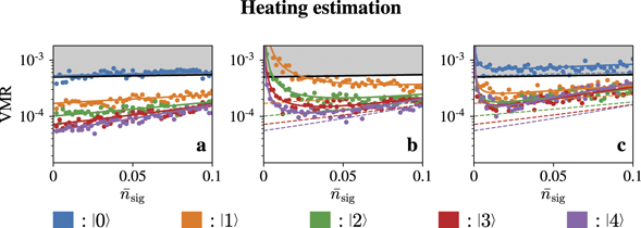
Figure I2. The simulated variance-to-mean ratios (VMRs) of mechanical heating estimations in the hypothetical situation, when the internal qubit measurement does not induce the photon recoil. The VMRs obtained from (a) the two-step measurement with negligible impurity and damping, (b) the two-step measurement with the probe being in the mixed state given in (F.3) with Ps = 0.9 and negligible damping, and (c) the two-step measurement with the damping coefficient γ0 = 0.02, as defined in (15). Different colors are used for different prepared Fock states  , n = 0, ..., 4.
Download figure:
Standard image High-resolution image