
Abstract
Quantum neural networks (QNNs) offer a powerful paradigm for programming near-term quantum computers and have the potential to speed up applications ranging from data science to chemistry to materials science. However, a possible obstacle to realizing that speed-up is the barren plateau (BP) phenomenon, whereby the gradient vanishes exponentially in the system size n for certain QNN architectures. The question of whether high-order derivative information such as the Hessian could help escape a BP was recently posed in the literature. Here we show that the elements of the Hessian are exponentially suppressed in a BP, so estimating the Hessian in this situation would require a precision that scales exponentially with n. Hence, Hessian-based approaches do not circumvent the exponential scaling associated with BPs. We also show the exponential suppression of higher order derivatives. Hence, BPs will impact optimization strategies that go beyond (first-order) gradient descent. In deriving our results, we prove novel, general formulas that can be used to analytically evaluate any high-order partial derivative on quantum hardware. These formulas will likely have independent interest and use for training QNNs (outside of the context of BPs).
Export citation and abstract BibTeX RIS
1. Introduction
Standard quantum algorithms were not developed to handle the constraints imposed by current quantum computers. Such noisy intermediate scale quantum (NISQ) devices have limited connectivity, limited qubit count, and noise that limits circuit depth.
On the other hand, training parameterized quantum circuits provides a promising approach for quantum computing in the NISQ era, as this approach adapts to the imposed constraints. Here, one utilizes a quantum computer to efficiently evaluate a cost (or loss) function  or its gradient
  , while employing a classical optimizer to train the parameters
θ
of a parameterized quantum circuit
, while employing a classical optimizer to train the parameters
θ
of a parameterized quantum circuit  . This strategy is employed in two closely related paradigms: variational quantum algorithms (VQAs) [1] for chemistry, optimization, and other applications [2–16], and quantum neural networks (QNNs) for classification applications [17–21]. QNNs can be viewed as a generalization of VQAs to the case of multiple input states, and thus we will henceforth use the term QNNs to encompass all methods that train parameterized quantum circuits.
While many novel QNNs have been developed, more rigorous scaling analysis is needed for these architectures. One of the few known results is the so-called barren plateau (BP) phenomenon [22–31], where the cost function gradient vanishes exponentially with the system size. This can arise due to deep unstructured ansatzes [22, 24, 30], global cost functions [23, 24], noise [25], or an excess of entanglement [27, 31]. Regardless of the origin, when a cost landscape exhibits a BP, one requires an exponential precision to determine a minimizing direction in order to navigate the landscape. Since the standard goal of quantum algorithms is polynomial scaling with the system size (in contrast to the exponential scaling of classical algorithms), the exponential scaling due to BP can destroy quantum speedup. Hence, the study and analysis of BPs should be viewed as a fundamental step in the development of QNNs to guarantee that they can, in fact, provide a speedup over classical algorithms.
Recently there have been multiple strategies proposed for avoiding BPs such as employing local cost functions [23, 28], pre-training [32], parameter correlation [33], layer-by-layer training [34], initializing layers to the identity [35], and employing problem-inspired ansatzes [36, 37]. These strategies are aimed at either avoiding or preventing the existence of a BP, and they appear to be promising, with more research needed on their efficacy on general classes of problems. In a recent article [38], an alternative idea was proposed involving a method for actually training inside and escaping a BP. Specifically, the proposal was to compute the Hessian H of the cost function, and the claim was that taking a learning rate proportional to the inverse of the largest eigenvalue of the Hessian leads to an optimization method that could escape the BP.
The question of whether higher-order derivative information (beyond the first-order gradient) is useful for escaping a BP is interesting and is the subject of our work here. Our main results are presented here in the form of two propositions and corollaries. First, we show that the matrix elements Hij of the Hessian are exponentially vanishing when the cost exhibits a BP. This implies that the calculation of Hij requires exponential precision. In our second result we show that the magnitude of any higher-order partial derivative of the cost will also be exponentially small in a BP. Our results suggest that optimization methods that use higher-order derivative information, such as the Hessian, will also face exponential scaling, and hence do not circumvent the scaling issues arising from BPs.
As a byproduct of our work, we derive novel formulas for higher-order partial derivatives of the cost function, which can be used to efficiently evaluate these derivatives on quantum hardware. These formulas are obtained via the so-called Pascal tree, which we also introduce here. Due to their generality, these formulas can be generically used for training parameterized quantum circuits. Higher-order derivative information can be useful for various applications such as chemistry [39] and solving partial differential equations [14], as well as characterizing landscapes [38] and improving optimization methods (e.g., Newton's method [40, 41]).
2. Preliminaries
To set the stage for our results, we first give some background on the cost function, the parameter shift rule, and BPs.
2.1. Cost function
In what follows, we consider the case when the cost can be expressed as a sum of expectation values:

where {ρx
} is a set (of size N) of input states to the parameterized circuit V(
θ
). In order for this cost to be efficiently computable, the number of states in the input set should grow at most polynomially with the number of qubits n, that is,  . In the context of QNNs, the states {ρx
} can be viewed as training data points, and hence (1) is a natural cost function for QNNs. In the context of VQAs, one typically chooses N = 1, corresponding to a single input state. In this sense, the cost function in (1) is general enough to be relevant to both QNNs and VQAs.
. In the context of QNNs, the states {ρx
} can be viewed as training data points, and hence (1) is a natural cost function for QNNs. In the context of VQAs, one typically chooses N = 1, corresponding to a single input state. In this sense, the cost function in (1) is general enough to be relevant to both QNNs and VQAs.
2.2. Parameter shift rule
Let θi
be an angle that parameterizes a unitary in V(
θ
) as  , with σi
a Hermitian operator with eigenvalues ±1. Then, the partial derivative
, with σi
a Hermitian operator with eigenvalues ±1. Then, the partial derivative  can be computed via the parameter shift rule [42, 43] as

Here,  denotes the indices distinct from i (i.e., the indices of parameters that are not being differentiated), and we define the notation

Note that the parameter shift rule in (2) allows one to exactly write the first-order partial derivative as a difference of cost function values evaluated at two different points. Moreover, we remark that equation (2) is not a finite difference formula, but rather corresponds to exactly evaluating the partial derivative.
2.3. Barren plateaus
As discussed in [22–31], by analyzing the scaling of the variance of the cost function partial derivative one can detect the presence of BPs in the cost function landscape. We denote this variance as Var θ [∂i C], where the expectation values in the variance are taken over θ . Specifically, when the cost function exhibits a BP one finds that Var θ [∂i C] is exponentially vanishing with the number of qubits, i.e.,

for some b > 1. Then, combining equation (4) with Chebyshev's inequality, the probability that the cost derivative deviates from its mean value (of zero [30]) is bounded as

for any c > 0. Equation (5) shows that, on average, the cost function partial derivatives will be exponentially small across the landscape, meaning that an exponential precision is needed to estimate the gradients and determine a cost minimizing direction.
BPs can arise due to multiple reasons. For instance, in the seminal work of [22] it was shown that deep unstructured circuits (i.e., random parametrized circuits with depths in  ) form 2-designs on n qubits and hence will have BPs. This phenomenon was later extended in [23] to the case of layered hardware efficient ansatzes where random two-qubit gates act on alternating pairs of qubits in a brick-like fashion. Therein it was shown that the existence of BPs is related to the locality of the operators Ox
in (1). Global operators Ox
that act non-trivially on all qubits have BPs irrespective of the depth of V(
θ
), while local operators which measure individual qubits will have BPs only for deep circuits. BPs were then identified in perceptron-based QNNs [24], and in tasks of learning scramblers [26]. Moreover, the BP phenomenon has also been linked to the presence of high levels of entanglement in the circuit [27, 31] and to the hardware noise acting throughout the computation [25].
) form 2-designs on n qubits and hence will have BPs. This phenomenon was later extended in [23] to the case of layered hardware efficient ansatzes where random two-qubit gates act on alternating pairs of qubits in a brick-like fashion. Therein it was shown that the existence of BPs is related to the locality of the operators Ox
in (1). Global operators Ox
that act non-trivially on all qubits have BPs irrespective of the depth of V(
θ
), while local operators which measure individual qubits will have BPs only for deep circuits. BPs were then identified in perceptron-based QNNs [24], and in tasks of learning scramblers [26]. Moreover, the BP phenomenon has also been linked to the presence of high levels of entanglement in the circuit [27, 31] and to the hardware noise acting throughout the computation [25].
In what follows, we formulate our main results irrespective of the mechanism that leads to the BP, and hence our results apply to all such mechanisms.
3. Hessian matrix elements
Let us now state our results of how the presence of BPs can affect the estimation of the Hessian. The Hessian H of the cost function is a square matrix whose matrix elements are the second derivatives of C( θ ), i.e.,

Reference [38] noted that the matrix elements of the Hessian can be written according to the parameter shift rule. Namely, one can first write

and then apply the parameter shift rule a second time:

Now, the second derivatives of the cost can be expressed as a sum of cost functions being evaluated at (up to) four points.
From the parameter shift rule we can then derive the following bound on the probability that the magnitude of the matrix elements |Hij | are larger than a given c > 0.
Proposition 1. Consider a cost function of the form (1), for which the parameter shift rule of (2) holds. Let Hij
be the matrix elements of the Hessian as defined in (7). Then, assuming that  , the following inequality holds for any c > 0,

Here ![${\mathrm{V}\mathrm{a}\mathrm{r}}_{\boldsymbol{\theta }}\left[{\partial }_{i}C\right]={\langle {\left({\partial }_{i}C\right)}^{2}\rangle }_{\boldsymbol{\theta }}-{\langle {\partial }_{i}C\rangle }_{\boldsymbol{\theta }}^{2}$](https://content.cld.iop.org/journals/2058-9565/6/3/035006/revision3/qstabf51aieqn10.gif) , where the expectation values are taken over
θ
.
, where the expectation values are taken over
θ
.
Proof. Equation (7) implies that the magnitudes of the Hessian matrix elements are bounded as

From Chebyshev's inequality we can bound the probability that the cost derivative deviates from its mean value (of zero) as

for all c > 0, and for all i. Then, let  be defined as the event that
  , where
  . Note that the set of events where |Hij
| ⩾ c is a subset of the set
. Note that the set of events where |Hij
| ⩾ c is a subset of the set  . Then, from the union bound and equation (11) we can recover (9) as follows:


where we used the fact that  . □
. □
Then, the following corollary holds
Corollary 1. Consider the bound in equation (12) of proposition 1. If the cost exhibits a BP, such that (4) holds, then the matrix elements of the Hessian are exponentially vanishing since

where  for some b > 1.
The proof follows by combining (9) and (4). Corollary 1 shows that when the cost landscape exhibits a BP, the matrix elements of the Hessian are exponentially vanishing with high probability. This implies that any algorithm that requires the estimation of the Hessian will requires a precision that grows exponentially with the system size.
4. Higher order partial derivatives
Let us now analyze the magnitude of higher order partial derivatives in a BP. We use the following notation for the | α |th-order derivative

where
α
is an |
α
|-tuple. Since one can take the derivative with respect to the same angle multiple times, we define the set Θ (of size M = |Θ|) as the set of distinct angles with respect to which we take the partial derivative. Similarly, let  be the compliment of Θ, so that
  . Then, for any Θk
∈ Θ we define Nk
as the multiplicity of Θk
in
α
such that
. Then, for any Θk
∈ Θ we define Nk
as the multiplicity of Θk
in
α
such that  . Since the cost function and any of its higher order partial derivatives are continuous function of the parameters (as can be seen below via multiple applications of the parameter shift rule), one can extend Clairaut's theorem [44] to rewrite

Then, applying the parameter shift rule | α | times we find that the | α |-order partial derivative can be expressed as a summation of cost functions evaluated at (up to) 2| α | points as

Here we defined  , with
  defined analogously to (3), and where

Also,
ω
= (ω1, ..., ωD
), where ωl
∈ {0, ±1} if Nl
is even, and  if Nl
is odd. Additionally, the coefficients
if Nl
is odd. Additionally, the coefficients  can be obtained from the Pascal tree which we introduce in figure 1. In the appendix
  and the Pascal tree.

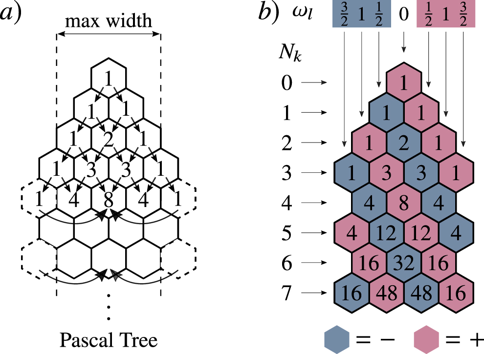
Figure 1. The Pascal tree. (a) The Pascal tree can be obtained by modifying how a Pascal triangle is constructed. In a Pascal triangle each entry of a row is obtained by adding together the numbers directly above to the left and above to the right, with blank entries considered to be equal to zero. The entries of a Pascal tree are obtained following the aforementioned rule, with the additional constraint that the width of the triangle is restricted to always being smaller than a given even number. Moreover, once an entry in a row is outside the maximum width, its value is added to the central entry in that row (see arrows). Here the maximum width is four. (b) The coefficients  in (20) can be obtained from the Pascal tree of (a) by adding signs to the entries of the tree. As schematically depicted, all entries in a diagonal going from top left to bottom right have the same sign, with the first entry in the first row having a positive sign. Here, each row corresponds to a given Nl
, while entries in a row correspond to different values of ωl
, with ωl
∈ {0, ±1} if Nl
is even, and
in (20) can be obtained from the Pascal tree of (a) by adding signs to the entries of the tree. As schematically depicted, all entries in a diagonal going from top left to bottom right have the same sign, with the first entry in the first row having a positive sign. Here, each row corresponds to a given Nl
, while entries in a row correspond to different values of ωl
, with ωl
∈ {0, ±1} if Nl
is even, and  if Nl
is odd. For instance,
if Nl
is odd. For instance,  .
.
Download figure:
Standard image High-resolution imageFrom (19) we obtain that the (| α | + 1)th-order derivative, which we denote as ∂i D α C( θ ) = Di, α C( θ ), is obtained as the sum of (up to) 2| α | partial derivatives:

Since one has to individually evaluate each term in (21) and since there are up to 2|
α
| terms, we henceforth assume that  . This guarantees that the computation of Di,
α
C(
θ
) leads to an overhead which is (at most)
. This guarantees that the computation of Di,
α
C(
θ
) leads to an overhead which is (at most)  .
.
The following proposition, which generalizes proposition 1, allows us to bound the probability that the magnitude of  is larger than a given c > 0.
Proposition 2. Consider a cost function of the form (1), for which the parameter shift rule of (2) holds. Let Di,
α
C(
θ
) be a higher order partial derivative of the cost as defined in (17). Then, assuming that  , the following inequality holds for any c > 0,

Proof. From equation (21) we can obtain the following bound

Let us define  as the event that
  . Since (4) holds, then the following chain of inequalities holds


where we invoked the union bound, and where we recall that  , ∀
ω
. In addition, for (27) we used the fact that the summation in (26) has at most 2|
α
| terms. □
, ∀
ω
. In addition, for (27) we used the fact that the summation in (26) has at most 2|
α
| terms. □
Then, if the cost function exhibits a BP, the following corollary follows.
Corollary 2. Consider the bound in equation (22) of proposition 2. If the cost exhibits a BP, such that (4) holds, then higher order partial derivatives of the cost function are exponentially vanishing since

where  for some q > 1.
Proof. Combining (4) and (22) leads to

Then, let us define G(n) = 2|
α
|
F(n). Since  , and
, and  , then we know that there exists κ, κ', and n0 such that ∀ n > n0 we, respectively, have 2|
α
| ⩽ nκ
and
, then we know that there exists κ, κ', and n0 such that ∀ n > n0 we, respectively, have 2|
α
| ⩽ nκ
and  . Combining these two results we find

where L(n) = (n − κ logb
(n)). Equation (30) shows that  . Then, since

we have L(n) ∈ Ω(n), meaning that there exists a  and
and  such that
  , we have
  . The latter implies
  for all
  , which means that
  where
where  . Also, q > 1 follows from b > 1 and
  .□
.□
Corollary 2 shows that, in a BP, the magnitude of any efficiently computable higher order partial derivative (i.e., any partial derivative where  ) is exponentially vanishing in n with high probability.
5. Discussion
In this work, we investigated the impact of BPs on higher order derivatives. As shown in [21, 38], information on these higher-order derivatives can be used to analyze the landscape of cost functions and shed some light on the relatively obscure nature of training landscapes for VQAs and QNNs. Moreover, it was also suggested that one could use higher order derivative information to escape a BP. We considered a cost function C that is relevant to both VQAs and QNNs, as BPs are relevant to both of these applications.
Our main result was that, when a BP exists, the Hessian and other high order partial derivatives of C are exponentially vanishing in n with high probability. Our proof relied on the parameter shift rule, which we showed can be applied iteratively to relate higher order partial derivatives to the first order partial derivative (analogous to what reference [38] did for the Hessian). Hence, the parameter shift rule allowed us to state the vanishing of higher order derivatives as essentially a corollary of the vanishing of the first order derivative. We remark that iterative applications of the parameter shift rule led us to a mathematically interesting construct that we called the Pascal tree, depicted in figure 1.
Our results imply that estimating higher order partial derivatives in a BP is exponentially hard. Hence, any optimization strategy that requires information about partial derivatives that go beyond first-order (such as the Hessian) will require a precision that grows exponentially with n. We therefore surmise that, by themselves, optimizers that go beyond first order gradient descent do not appear to be a feasible solution to the BP problem. More generally, our results suggest that it is better to develop strategies that avoid the appearance of the BP altogether, rather than to try to escape an existing BP.
Finally, we remark that our results were derived using equation (21) and the Pascal tree, which provide novel, general formulas for arbitrary higher-order partial derivatives of the cost function in equation (1). These formulas are of interest on their own, as they can be generically employed to analytically evaluate higher-order derivatives of the cost on quantum hardware. As an example application, one could apply this method to take derivatives of quantum feature maps for solving partial differential equations [14].
While some prior work on higher-order derivative formulas was performed in reference [45], our formulas are more explicit and our introduction of the Pascal tree is novel. We also remark that, in a recent post that was concurrent with our work, reference [41] introduced a formula similar to equation (21) for explicitly determining higher-order partial derivatives, albeit that work analyzes the formulas in a different context.
Acknowledgments
We thank Kunal Sharma for helpful discussions. Research presented in this article was supported by the Laboratory Directed Research and Development program of Los Alamos National Laboratory under project number 20180628ECR. MC was also supported by the Center for Nonlinear Studies at LANL. PJC also acknowledges support from the LANL ASC Beyond Moore's Law project. This work was also supported by the U.S. Department of Energy (DOE), Office of Science, Office of Advanced Scientific Computing Research, under the Accelerated Research in Quantum Computing (ARQC) program.
Data availability statement
No new data were created or analysed in this study.
Appendix A.: Explicit description of 

In this appendix we first discuss how the parameter shift rule leads to the Pascal tree. Then, we provide analytical formulas for  .
.
Let us consider the first and second order partial derivatives of the cost function with respect to the same angle. From the parameter shift rule of equation (2) we find

where we can see that  . Similarly, if we were to take the third partial derivative with respect to i we would find |d(±1/2,3)| = |d(0,2)| + |d(±1,2)|, and |d(±3/2,3)| = |d(±1,2)|. Note that this procedure forms the first four rows of the Pascal tree, which actually coincide with first four rows of the Pascal triangle. When taking the fourth partial derivative we have to take into account the fact that
  , since e−iθσ/2 is equal to e−i(θ+2π)σ/2 up to an unobservable global phase. Hence, the fact that θ ≡ θ(2)(mod 2π) imposes a restriction on the width of the Pascal tree. Hence, following this procedure one can recover the entries in figure 1.
For arbitrary ωl
and Nl
, the coefficients  can be analytically obtained as follows: If Nk
< 2 we have d(±1,0) = 0,
can be analytically obtained as follows: If Nk
< 2 we have d(±1,0) = 0,  , d(±1/2,1) = ±1, and d(±3/2,1) = 0. Then, for Nk
⩾ 2
, d(±1/2,1) = ±1, and d(±3/2,1) = 0. Then, for Nk
⩾ 2

Note that ∀ Nl
we have  .
.