
Abstract
Graph states are ubiquitous in quantum information with diverse applications ranging from quantum network protocols to measurement based quantum computing. Here we consider the question whether one graph (source) state can be transformed into another graph (target) state, using a specific set of quantum operations (LC + LPM + CC): single-qubit Clifford operations (LC), single-qubit Pauli measurements (LPM) and classical communication (CC) between sites holding the individual qubits. This question is of interest for effective routing or state preparation decisions in a quantum network or distributed quantum processor and also in the design of quantum repeater schemes and quantum error-correction codes. We first show that deciding whether a graph state |G⟩ can be transformed into another graph state |G'⟩ using LC + LPM + CC is  -complete, which was previously not known. We also show that the problem remains NP-complete even if |G'⟩ is restricted to be the GHZ-state. However, we also provide efficient algorithms for two situations of practical interest. Our results make use of the insight that deciding whether a graph state |G⟩ can be transformed to another graph state |G'⟩ is equivalent to a known decision problem in graph theory, namely the problem of deciding whether a graph G' is a vertex-minor of a graph G. The computational complexity of the vertex-minor problem was prior to this paper an open question in graph theory. We prove that the vertex-minor problem is
  -complete by relating it to a new decision problem on 4-regular graphs which we call the semi-ordered Eulerian tour problem.
Export citation and abstract BibTeX RIS

Original content from this work may be used under the terms of the Creative Commons Attribution 4.0 licence. Any further distribution of this work must maintain attribution to the author(s) and the title of the work, journal citation and DOI.
1. Introduction
A key concept in realizing quantum technologies is the preparation of specific resource states, which then enable further quantum processing. For example, many quantum network protocols first ask to prepare a specific resource state that is shared amongst the network nodes, followed by measurements and exchange of classical communication (CC). The simplest instance of this concept is indeed quantum key distribution [3, 21], in which we first produce a maximally entangled state, followed by random measurements. Similarly, measurement-based quantum computing [41] proceeds by first preparing the quantum device in a large resource state, followed by measurements on the qubits.
An important class of such resource states are graph states. These states can be described by a simple undirected and unweighted graph where the vertices correspond to the qubits of the state [29]. The graph state of a given graph is formed by initializing each qubit v ∈ V(G) in the state  and for each edge (u, v) ∈ E(G) applying a controlled phase gate between qubits u and v. Apart from their broad range of applications, an appealing feature of graph states is that they can be efficiently described classically. Specifically, to describe a graph state on n qubits, only
  bits are needed to specify the edges of the graph. This is in sharp contrast to the 2n
complex numbers required to describe a general quantum state [38]. It turns out that for graph states, and indeed the more general class of stabilizer states, their evolution under Clifford operations and Pauli measurement can be simulated efficiently on a classical computer [28].
bits are needed to specify the edges of the graph. This is in sharp contrast to the 2n
complex numbers required to describe a general quantum state [38]. It turns out that for graph states, and indeed the more general class of stabilizer states, their evolution under Clifford operations and Pauli measurement can be simulated efficiently on a classical computer [28].
Well-known applications of graph states include cluster states [37] used in measurement based quantum computing where, together with arbitrary single-qubit measurements, these states form a universal resource for measurement-based quantum computation [41]. Graph states also arise as logical codewords of many error-correcting codes [44]. In the domain of quantum networking, a specific class of graph states is of particular interest. Specifically, these are states which are GHZ-like, i.e., they are equivalent to the GHZ-state up to single-qubit Clifford operations. GHZ-states have been shown to be useful for applications such as quantum secret sharing [35], anonymous transfer [12], conference key agreement [42] and clock synchronization [31]. It turns out that graph states described by either a star graph or a complete graph are precisely those GHZ-like states [29].
Given the desire for graph states, we may thus ask how they can effectively be prepared, and transformed. We consider the situation in which we already have a specific starting state (the source state), and we wish to transform it to a desired target state, using an available set of operations. Motivated by the fact that on a quantum network or distributed quantum processor, local operations are typically much faster and easier to implement, we consider the set of operations consisting of single-qubit Clifford operations (LC), single-qubit Pauli measurements (LPM), and CC. Applications of an efficient algorithm that finds a series of operations to transform a source to a target state includes the ability to make effective routing decisions for state preparation on a distributed quantum processor or network. Here, fast decisions are essential since quantum memories are inherently noisy and the source state will therefore become useless if too much time is spent on making a decision. Such algorithms could also be used as a design tool in the study of quantum repeater schemes [1], and the discovery of effective code switching procedures in quantum error correction [27, 36].
1.1. Previous work
It turns out that single-qubit Clifford operations on graph states correspond to an operation called local complementation [9] on the corresponding graph [48]. Furthermore, single-qubit Pauli measurements and CC correspond to local complementations and vertex-deletions [29]. The graphs reachable from G by performing local complementations and vertex-deletions are called vertex-minors of G. Vertex-minors are well-studied objects in graph theory [39]. To understand which graph states are related under LC + LPM + CC operations we introduced the notion of a qubit-minor in [18]. A qubit-minor of a graph state |G⟩ is another graph state |G'⟩ such that |G⟩ can be transformed to |G'⟩ using only LC + LPM + CC operations. We show in [18] that the notion of qubit-minors is equivalent to the notion of vertex-minors, in the sense that the graph state |G'⟩ is a qubit-minor of |G⟩ if and only if the graph G' is a vertex-minor of G.
Vertex-minors play an important role in algorithmic graph theory, together with the notion of rank-width, which is a complexity measure on graphs. Specifically, one can efficiently decide membership of a graph in some set of graphs, if this set is closed under taking vertex-minors and of fixed (bounded) rank-width [39]. An example of such a set is the set of distance-hereditary graphs, which are exactly the graphs with rank-width one [39]. Another example of a set of graphs which is closed under taking vertex-minors are circle graphs, which are however of unbounded rank-width ([40, proposition 6.3] and [13]). An appealing connection between the rank-width of graphs, and the entanglement in the corresponding graph states was identified in [49], where it is shown that the rank-width of a graph equals the Schmidt-rank width of the corresponding graph state. The Schmidt-rank width of a quantum state is an entanglement measure. Specifically, the higher rank-width a graph has, the more entanglement there is in the corresponding graph state, in terms of this measure. Another interpretation of the Schmidt-rank width is that it captures how complex the quantum state is. One reason for this interpretation is that quantum states can be described using a technique called tree-tensor networks and it was shown in [49] that the minimum dimension of the tensors needed to describe a state is in fact given by the Schmidt-rank width.
In the domain of complexity theory, the rank-width and related measures such as the tree- and clique-width [4, 15] also form a measure of the inherent complexity of instances to graph problems, and feature prominently in the study of fixed-parameter tractable (FPT) algorithms [20]. Specifically, a problem is called FPT in terms of a parameter r, if any instance I of the problem of fixed r, is solvable in time  , where |I| is the size of the instance and f is a computable function of r [20]. In this work, r is the rank-width, and for graphs of constant rank-width the techniques of Courcelle [16] and its generalizations [14], can be used to obtain polynomial time algorithms for problems such as graph coloring [24], or Hamiltonian path [34]. While very appealing from a complexity theory point of view, a direct application of these techniques does not usually lead to polynomial time algorithms that are also efficient in practice, since f(r) is often prohibitively large.
Since the problem of deciding whether a graph state |G'⟩ is a qubit-minor of |G⟩ (QUBITMINOR) is equivalent to deciding if G' is a vertex-minor of G (VERTEXMINOR) [18], an efficient algorithm for VERTEXMINOR directly provides an efficient algorithm for QUBITMINOR. This in turn can be used for fast decisions on how to transform graph states in a quantum network or distributed quantum processor. However, not much was previously known about the computational complexity of VERTEXMINOR and therefore whether efficient algorithms exists. For a related but slightly more restrictive minor-relation, namely pivot-minors it has been shown in [17] that checking whether a graph G has a pivot-minor isomorphic to another graph G' is  -complete. However the complexity of deciding whether G' is a vertex-minor of G was left as an open problem. We emphasize that for our application we are interested in preparing a specific target state G' on a specific set of qubits, as qubits are generally not interchangeable in the applications of our algorithm. As such, our question is not whether we can obtain a graph that is isomorphic to G', but rather whether we can obtain G' on a specific set of vertices.
Evidently, for fixed rank-width, it is not difficult to apply the techniques of Courcelle [16], to obtain an FPT algorithm for our problem that is efficient if both the size of G', as well as the rank-width of G are bounded (as we have shown in [18]). Indeed, a powerful method for deciding if a graph problem is FPT is by Courcelle's theorem and its generalizations [14]. It turns out that also for our case, a direct implementation of Courcelle's theorem does not give an algorithm that can be used in practice. In fact, in the case of VERTEXMINOR, this constant factor obtained by applying the techniques of Courcelle in [18] can be shown to be a tower of twos

where r is the rank-width of the input graph G and the height of the tower is 10 [18].
1.2. Results and proof techniques
In this paper we determine the computational complexity of VERTEXMINOR and therefore of QUBITMINOR. In particular we prove that it is in general  -complete to decide whether a graph G' is a vertex-minor of another graph G. We however also give efficient algorithms for this problem whenever the input graphs belong to particular graph classes. An overview of the complexity of the problem for different classes of graphs considered in this paper can be seen in figure 1.

Figure 1. An overview of the graph classes discussed in this paper and what the computational complexities of solving STARVERTEXMINOR on these classes are. The sizes of the sets in the figure are not exact, however their intersections and non-intersections are.
Download figure:
Standard image High-resolution imageWe point out that our results of  -completeness and the presented algorithms also apply to the more general class of stabilizer states of relevance in quantum error correction. This is because any stabilizer state can be transformed to some graph state using only single-qubit Clifford operations. Furthermore, given a stabilizer state on n qubits, a graph state equivalent under single-qubit Clifford operations can be found efficiently in time
  [48].
[48].
Below we list the main results and proof techniques of this paper. Our first result is a proof that VERTEXMINOR and QUBITMINOR are both  -complete.
Theorem 1.1 (Informal). The problem of deciding whether a graph G' is a vertex-minor of another graph G is  -complete. This implies that QUBITMINOR is also
  -complete. ◊
Our study of QUBITMINOR and VERTEXMINOR is motivated by the fact that efficient algorithms that solve these problems can be used to make for example routing decisions in a quantum network. Unfortunately theorem 1.1 tells us that no such algorithms exist, unless  =
=  . However, along with the proof of
  -completeness we also provide efficient algorithms for the following three restricted variants of VERTEXMINOR and QUBITMINOR:
- (a)Decide if a star graph on vertices V' is a vertex-minor of a distance-hereditary graph G. This is equivalent to deciding if the GHZ-state on qubits V' is a qubit-minor of a graph state |G⟩ with Schmidt-rank width one.
- (b)For a fixed k, decide if a star graph on vertices V', where |V'| ⩽ k, is a vertex-minor of a circle graph G. This corresponds to deciding if a GHZ-state of bounded size on qubits V' is a qubit-minor of a circle graph state |G⟩ with unbounded entanglement.
- (c)Decide if a graph G' on vertices V', where |V'| ⩽ 3 is a vertex-minor of a graph G.
For a visual overview of these different graph classes see figure 1 and for more details section 2. We will from now on denote the special case of VERTEXMINOR where G' is restricted to be a star graph as STARVERTEXMINOR.
Theorem 1.2 (Informal). The algorithm presented in section 4.1.1, consisting of algorithms 1 and 2, solves STARVERTEXMINOR in time  and is correct if G is distance-hereditary, or equivalently if G has rank-width one. ◊
Algorithm 1. Producing SV' from a distance-hereditary graph G.
| 1: INPUT: A graph G and a subset of vertices V' ⊆ V(G). | |
| 2: OUTPUT: A sequence v such that τ v (G)[V'] = SV', if SV' < G. | |
| 3: ERROR, if SV' ≮ G. | |
| 4: __________________________________________________________________________________________ | |
| 5: | |
| 6: if |V'| = 1 then | |
| 7: Return () | |
| 8: QUIT | |
| 9: end if | |
| 10: Find a v such that τ v (G) contain the star graph on V' as a subgraph by calling algorithm 2. | |
| 11: Let c be a vertex in V', adjacent to all other in V' (except itself). | |
| 12: for i in {0, 1} do (⊳) Two iterations are always needed if there is more than one bad edge | |
| 13: Let B be the vertices incident to a bad edge. (⊳) These are the vertices in τm (G)[V'\{c}] of degree 1 or higher | |
| 14: Let L = V'\({c} ∪ B). | |
| 15: if B = ∅ then (⊳) If already SV', only for i = 0 | |
| 16: Return v | |
| 17: QUIT | |
| 18: else | |
| 19: if B = V'\{c} then (⊳) I.e. if L = ∅ | |
| 20: Set v = v ||(c) | |
| 21: BREAK | |
| 22: end if | |
| 23: Let U be the set U = {u ∈ V(G)\V' : B ⊆ Nu ∧ L ⊈ Nu } (⊳) Candidates for the u in equation (105) | |
| 24: if U = ∅ then | |
| 25: Raise ERROR(SV' is not a vertex-minor of G) (⊳) Actually not needed, only for clarity | |
| 26: end if | |
| 27: Set found = False | |
| 28: for u in U do | |
| 29: if (u, c) ∉ E(τ v (G)) then | |
| 30: Set v = v ||(u) | |
| 31: Set found = True (⊳) Found a u satisfying equation (105) | |
| 32: Break | |
33: else if
 then
then
| |
| 34: Set v = v ||(h, u) | |
| 35: Set found = True (⊳) Found a u and h satisfying equation (105) | |
| 36: Break | |
| 37: end if | |
| 38: end for | |
| 39: if ¬found then (⊳) I.e. condition equation (105) is false | |
| 40: Raise ERROR (SV' is not a vertex-minor of G) | |
| 41: end if | |
| 42: end if | |
| 43: end for | |
| 44: Return v | |
| 45: QUIT |
Algorithm 2. Find a v such that τ v (G) contain the star graph on V' as a subgraph.
| 1: INPUT: A graph G and a subset of vertices V' ⊆ V(G). | |
| 2: OUTPUT: A sequence v such that τ v (G)[V'] = SS(B,L,c), where (B, L, {c}) is a partition of V'. | |
| 3: _____________________________________________________________________________________________________ | |
| 4: | |
| 5: Pick an arbitrary vertex from V' and denote this f | |
| 6: Find a v such that τ v (G)[V'\{f}] = SV' and denote the center c by calling algorithm 1 | |
| 7: Find a shortest path P = (p0 = f, p1, ⋯, pk , pk+1 = c) between f and c. | |
| 8: for i in (1, ⋯, k) do | |
| 9: if f is adjacent to any vertex in V'\{c} in the graph τ v (G) then | |
| 10: Pick an arbitrary vertex in Nf (τ v (G)) ∩ V'\{c} and denote this v | |
| 11: Set v = v ||v | |
| 12: else | |
| 13: Set v = v ||(f, pi , f) | |
| 14: end if | |
| 15: end for | |
| 16: Return v | |
| 17: QUIT |
The algorithm mentioned in the above theorem can therefore be used to decide how to transform graph states, with Schmidt-rank width one, to GHZ-states using single-qubit Clifford operations, single-qubit Pauli measurements and CC. As mentioned above, a more general method to find efficient algorithms for certain graph problems on graphs with bounded rank-width is by using Courcelle's theorem [14]. Compared to the algorithm provided by a direct implementation of Courcelle's theorem, see [18], our algorithm presented here does not suffer from a huge constant factor in the runtime, as in equation (1). In fact, besides providing proof for correctness and runtime, we have also implemented the algorithm [1] and see that it typically takes for example 50 ms to run for the case when |V(G)| = 50 on a standard desktop computer, see figure 2.

Figure 2. Average and maximal observed run-times for two algorithms that check if a GHZ-state on four qubits is a qubit-minor of a randomly generated connected graph state |G⟩ on qubits V of Schmidt-rank width 1. Random connected graph states of Schmidt-rank width 1 are generated by starting from a single-qubit graph and randomly adding leaves or performing twin-splits, see section 2.5.1, which generates any connected graph state of Schmidt-rank width 1 [2]. 'Our alg.' refers to the algorithm described in section 4.1.1 and 'Brute' is the non-efficient algorithm described in [18]. The algorithm of [18] based on the techniques of Courcelle [16] is not depicted here since the pre-factor makes an application impractical in practice whenever |V| < f(r) of equation (1). For each size of V, 10 random graph states are generated for 'Brute' and 100 random graph states for 'Our alg.', from which the average '(avg.)' and max '(max)' runtime is computed. Both algorithms are implemented in SAGE [46] and the tests were performed on an iMac with 3.2 GHz Intel Core i5 processor with 8 GB of 1600 MHz RAM.
Download figure:
Standard image High-resolution imageDistance-hereditary graphs, and therefore graphs with rank-width one, are exactly the graphs that can be reached by adding leaves and performing twin-splits from a graph with one vertex [2]. To prove that our algorithm is correct we also present some new interesting results relating vertex-minors, distance-hereditary graphs and leaves and twins. For example we show that if v is a leaf or a twin in G but not a vertex in G', then G' is a vertex-minor of G if and only if G' is a vertex-minor of G\v, where \v denotes vertex-deletion.
We call k-STARVERTEXMINOR the restriction of STARVERTEXMINOR where G' is restricted to a star graph having k vertices, corresponding to a GHZ-state (up to LC) on k qubits.
Theorem 1.3 (Informal).
k-STARVERTEXMINOR is in  if G is a circle graph
2
.
if G is a circle graph
2
.
The above theorem implies that STARVERTEXMINOR is FPT in the size of G' on circle graphs. Interestingly the class of circle graphs has unbounded rank-width ([40, proposition 6.3] and [13]) and the corresponding graph states therefore have unbounded entanglement according to the Schmidt-rank width. Thus, theorem 1.3 is not captured by the results from Courcelle [14] and implies that efficient algorithms can be found even on graphs with unbounded rank-width.
Theorem 1.4 (Informal). Any connected graph G' on three vertices or less is a vertex-minor of any connected graph G if and only if the vertices of G' are also in G. ◊
Along with the above theorem we also provide an efficient algorithm for finding the transformation that takes the former graph to the latter.
We show this result by first proving that G has a vertex-minor which is connected, on any subset of its vertices. Then from the fact that there is only a single equivalence class for graphs on one, two or three vertices, respectively, under the considered operations, the result follows.
Along with the mentioned theorems we also prove several theorems needed for the main results that may be interesting in their own right. For example we prove the following theorem which points out an interesting behavior of bipartitions of vertices of a graph.
Theorem 1.5 (Informal). Assume G is a graph on the vertices U ∪ L such that U ∩ L = ∅ and U ≠ ∅. Furthermore, assume that for each l in L, there is at least one vertex in U not adjacent to l and for each u in U, there is at least one vertex in L adjacent to u. Then there exist two vertices u1 and u2 in U and two vertices l1 and l2 in L such that u1 is adjacent to l1 but not to l2 and u2 is adjacent to l2 but not to l1. ◊
In section 2.5 we introduce the notion of a foliage which is the set of leaves, axils and twins in a graph and prove the following theorem.
Theorem 1.6 (Informal). Any distance-hereditary graph on more than four vertices has a foliage (the set of leaves, axils and twins in the graph) of size at least four. ◊
As mentioned, we prove that STARVERTEXMINOR is NP-complete on a strict subclass of circle graphs
3
and that STARVERTEXMINOR is in  on distance-hereditary graphs. These two graph classes are in fact disjoint, which we prove in the following theorem.
Theorem 1.7 (Informal). No circle graph induced by a Eulerian tour on a triangular expansion of some 3-regular graph is distance-hereditary. ◊
1.3. Overview
The paper is structured as follows. In section 2 we describe graph states and consider several notions of graph theory we will need throughout the paper. We also introduce the VERTEXMINOR and STARVERTEXMINOR problems and the notion of a semi-ordered Eulerian tour (SOET). We also prove a few technical results concerning distance-hereditary graphs, circle graphs and vertex-minors which we will need later. Formal statement and proof of theorem 1.1 above is given in section 3 (as theorem 3.1), theorem 1.2 in section 4.1, theorem 1.3 in section 4.2 (as corollary 4.7.1) and theorem 1.4 in section 5 (as theorem 5.1). In section 3 we consider the computational complexity of the VERTEXMINOR and STARVERTEXMINOR problems. In particular we prove that both problems are  -complete (result 1). We also define the SOET problem and prove that it is
  -complete as well. In section 4 we provide an efficient algorithm for STARVERTEXMINOR when the input graph is restricted to be distance-hereditary and prove that it is correct (result 2). We also provide a FPT algorithm for STARVERTEXMINOR when the input graph is a circle graph and prove its correctness (result 3). Finally we prove that any connected graph G' with three or less vertices is a vertex-minor of any connected graph G if V(G') ⊆ V(G) and provide an efficient algorithm for finding the transformation that takes the former graph to the latter (result 4).
2. Preliminaries
In this section we set our notation and recall various concepts which will be used throughout the rest of the paper. We start by providing the definitions of graph states, qubit-minors and the relation to vertex-minors. We then recall the definitions of local complementation and vertex deletion as operations on graphs. These operations are useful in the context of graph states since they completely capture the action of LC + LPM + CC on graph states. Furthermore, we discuss circle graphs and their various characterizations and discuss how local complementation behaves on these graphs. We also introduce the concept of semi-ordered Eulerian tours, which is a key technical concept for the results later in this paper. Finally we discuss distance-hereditary graphs, which form a subclass of circle graphs. We discuss how these graphs can be built up out of elementary pieces and prove some technical results which will be used later.
2.1. Notation and definitions
Here we introduce some notation and vocabulary that will be used throughout this paper. We assume familiarity of the general notation of quantum information theory, see [38] for more details.
Quantum operations. The Pauli matrices will be denoted as

The single-qubit Clifford group  consists of operations which leave the Pauli group
  invariant. More formally,
  is the normalizer of the Pauli group, i.e.

where  is the single-qubit unitary operations.
Sequences and words. A sequence
X
= x1
x2⋯xk
is an ordered, possibly empty, tuple of elements in some set X. We also call a sequence a word and its elements letters. We write
X
⊆ X, when all letters of
X
are in the set X. A sub-word
X
' of
X
, is a word which can be obtained from
X
by iteratively deleting the first or last element of
X
. We denote the concatenation of two words  and
and  as
as  . We also denote the 'mirror image' by an overset tilde, e.g. if
X
= ab then
. We also denote the 'mirror image' by an overset tilde, e.g. if
X
= ab then  .
.
Sets. The set containing the natural numbers from 1 to n is denoted [n]. The symmetric difference XΔY between two sets X and Y is the set of elements of X and Y that occur in X or Y exclusively, i.e. XΔY = (X ∪ Y)\(X ∩ Y).
Graphs. A simple undirected graph G = (V, E) is a set of vertices V and a set of edges E. Edges are 2-element subsets of V for simple undirected graphs. Importantly, we only consider labeled graphs, i.e. we consider a complete graph with vertices {1, 2, 3} to be different from a complete graph with vertices {2, 3, 4}, even though these graphs are isomorphic. The reason for considering labeled graphs is that these will be used to represent graph states on specific qubits, possibly at different physical locations in the case of a quantum network. In a simple undirected graph, there are no multiple edges or self-loops, in contrast with a multi-graph: An undirected multi-graph H = (V, E) is a set of vertices V and a multi-set of edges E. For undirected multi-graphs, edges are unordered pairs of elements in V. We will often write V(G) = V and E(G) = E to mean the vertex- and edge-set of the (multi-)graph G = (V, E).
Next we list some glossary about (multi-)graphs:
- If a vertex v ∈ V is an element of an edge e ∈ E, i.e. v ∈ e, then v and e are said to be incident to one another.
- Two vertices which are incident to a common edge are called adjacent.
- The set of all vertices adjacent to a given vertex v in a (multi-)graph G is called the neighborhood
 of v. We will sometimes just write Nv
if it is clear which (multi-)graph is considered.
of v. We will sometimes just write Nv
if it is clear which (multi-)graph is considered. - The degree of a vertex v is the number of neighbors of v, i.e. |Nv |.
- A k-regular (multi-)graph is a (multi-)graph such that every vertex in the (multi-)graph has degree k.
- A walk W = v1 e1 v2⋯ek vk+1 is an alternating sequence of vertices and edges such that ei is incident to vi and vi+1 for i ∈ [k].
- The vertices v1 and vk+1 are called the ends of W.
- If the ends of a walk are the same vertex, it is called closed.
- A trail is a walk which does not include any edge twice.
- A closed trail is called a tour.
- A path is a walk which does not include any vertex twice, apart from possibly the ends.
- A closed path is called a cycle.
- Two vertices u and v are called connected if there exists a path with u and v as ends.
- A (multi-)graph is called connected if any two vertices are connected in the (multi-)graph.
- G' = (V', E') is a subgraph of G = (V, E) if V' ⊆ V and E' ⊆ E.
- An induced subgraph
G[V'] of G = (V, E) is a subgraph on a subset V' ⊆ V and with the edge-set
- A connected component of a (multi-)graph G = (V, E) is a connected induced subgraph G[V'] such that no vertex in V' is adjacent to a vertex in V\V' in the (multi-)graph G.
- A cut-vertex v of a (multi-)graph G = (V, E) is a vertex such that G[V\{v}] has strictly more connected components than G
- The distance dG (v, w) between two vertices v, w in a (multi-)graph G is equal to the number of edges in the shortest path that connects v and w.
- The complement
GC
of a graph G = (V, E) is a graph with vertex-set VC
= V and edge-set


A graph G is assumed to be simple and undirected, unless specified and will be denoted as G, Gi
, G',  or similar. A multi-graph is assumed to be undirected, unless specified and will be denoted as H, Hi
, H',
or similar. A multi-graph is assumed to be undirected, unless specified and will be denoted as H, Hi
, H',  or similar. Furthermore, 3-regular simple graphs will be denoted as R, Ri
, R' or similar and 4-regular multi-graphs as F, Fi
, F' or similar. We will denote the complete graph on a set of vertices V as KV
and the star graph on a set of vertices V with center c by SV,c
. We will often not care about the choice of center, writing SV
to mean any choice of star graph on the vertex set V.
or similar. Furthermore, 3-regular simple graphs will be denoted as R, Ri
, R' or similar and 4-regular multi-graphs as F, Fi
, F' or similar. We will denote the complete graph on a set of vertices V as KV
and the star graph on a set of vertices V with center c by SV,c
. We will often not care about the choice of center, writing SV
to mean any choice of star graph on the vertex set V.
2.2. Graph states
A graph state is a multi-partite quantum state |G⟩ which is described by a graph G, where the vertices of G correspond to the qubits of |G⟩. The graph state is formed by initializing each qubit v ∈ V(G) in the state  and for each edge (u, v) ∈ E(G) applying a controlled phase gate between qubits u and v. Importantly, all the controlled phase gates commute and are invariant under changing the control- and target-qubits of the gate. This allows the edges describing these gates to be unordered and undirected. Formally, a graph state |G⟩ is given as

where  is a controlled phase gate between qubit u and v, i.e.

and Zv is the Pauli-Z matrix acting on qubit v.
Any graph state is also a stabilizer state [29]. The GHZ states are an important class of stabilizer states given as

It is easy to verify that any graph state given by a star or complete graph, i.e. |SV,c ⟩ or |KV ⟩, can be turned into a GHZ state on the qubits V using only single-qubit Clifford operations. Furthermore, it is easy to see 4 no other graph states are single-qubit Clifford equivalent to the GHZ-states.
In the next section we discuss local complementations and vertex-deletions on graph states. It turns out that single-qubit Clifford operations (LC), single-qubit Pauli measurements (LPM) and CC: LC + LPM + CC, which take graph states to graph states, can be completely characterized by local complementations and vertex-deletions on the corresponding graphs. More concretely, any sequence of single-qubit Clifford operations, mapping graph states to graph states, can be described as some sequence of local complementations on the corresponding graph. Moreover, measuring qubit v of a graph state |G⟩ in the Pauli-X, Pauli-Y or Pauli-Z basis, gives a stabilizer state that is single-qubit Clifford equivalent to |Xv (G)⟩, |Yv (G)⟩, |Zv (G)⟩ respectively. The operations Xv , Yv and Zv are graph operations consisting of sequences of local complementations together with the deletion of vertex v, which we define in definition 2.6. As mentioned the post-measurement state of for example a Pauli-X measurement on qubit v is only single-qubit Clifford equivalent to the graph state |Xv (G)⟩. The single-qubit Clifford operations that take the post-measurement state to |Xv (G)⟩ depend on the outcome of the measurement of the qubit v and act on qubits adjacent to v [29]. This means CC is required to announce the measurement result at the vertex v to its neighboring vertices.
In [18] we introduced to notion of a qubit-minor which captures exactly which graph states can be reached from some initial graph state under LC + LPM + CC. Formally we define a qubit-minor as:
Definition 2.1 (Qubit-minor). Assume |G⟩ and |G'⟩ are graph states on the sets of qubits V and U respectively. |G'⟩ is called a qubit-minor of |G⟩ if there exists an adaptive sequence of single-qubit Clifford operations (LC), single-qubit Pauli measurements (LPM) and CC that takes |G⟩ to |G'⟩, i.e.

If |G'⟩ is a qubit-minor of |G⟩, we denote this as

◊
In [18] we have shown that the notion of qubit-minors for graph states is equivalent to the notion of vertex-minors for graphs. We will define and discuss vertex-minors in section 2.3.1, however we formally state the relation between vertex-minors here. For a proof see [18].
Theorem 2.1. (Theorem 2.2 in [18]). Let |G⟩ and |G'⟩ be two graph states such that no vertex in G' has degree zero. Then |G'⟩ is a qubit-minor of |G⟩ if and only if G' is a vertex-minor of G, i.e.

◊
Note that one can also include the case where G' has vertices of degree zero. Let us denote the vertices of G' which have degree zero as I. We then have that

Theorem 2.1 is very powerful since it allows us to consider graph states under LC + LPM + CC, purely in terms of vertex-minors of graphs. We will therefore in the rest of this paper use the formalism of vertex-minors to study the computational complexity of transforming graph states using LC + LPM + CC and provide efficient algorithms for transforming graph state using LC + LPM + CC.
2.3. Local complementations and vertex-deletions
Local complementation is a fundamental operation on graphs [9]. This operation has found applications in quantum information theory since it has been shown that two graph states |G⟩ and |G'⟩ are equivalent under single-qubit Clifford operations if and only if the graphs G and G' are related by some sequence of local complementations [47]. We have the following definition.
Definition 2.2 (Local complementation). A local complementation τv is a graph operation specified by a vertex v, taking a graph G to τv (G) by replacing the induced subgraph on the neighborhood of v, i.e. G[Nv ], by its complement. The neighborhood of any vertex u in the graph τv (G) is therefore given by

where Δ denotes the symmetric difference between two sets. Given a sequence of vertices v = v1⋯vk , we denote the induced sequence of local complementations, acting on a graph G, as

◊
Below we show a simple example of the action of local complementation on a graph (in particular we consider a local complementation on the vertex labeled 2).

If two graphs G1 and G2 are related by a sequence of local complementations, i.e. ∃
v
: τ
v
(G1) = G2, we call the two graphs LC-equivalent and denote this as G1 ∼ LC
G2. Checking whether two graphs are LC-equivalent can be done in time  , where n is the size of the graphs, as shown in [10]. This result was used in [47] to find an efficient algorithm for checking whether two graph states are equivalent under single-qubit Clifford operations, by proving that two graph states are equivalent under single-qubit Cliffords if and only if their corresponding graphs are LC-equivalent.
Notable about local complementation is its action on star and complete graphs. For a vertex set V and c ∈ V we have that τc (SV,c ) = KV and for any v ∈ V we have τv (KV ) = SV,v . This means all star graphs on a vertex set V are equivalent to each other under local complementation and also to the complete graph on V. Moreover, no other graph is equivalent to the star or complete graph.
Another operation which we will make use of is the pivot.
Definition 2.3 (Pivot). A pivot ρe is a graph operation specified by an edge e = (u, v), taking a graph G to ρe (G) such that

◊
The pivot can simply be specified by an undirected edge since

as shown in [7].
It will be useful to be able to specify a pivot simply by a vertex v. We therefore also introduce the following definition:
Definition 2.4. The graph operation ρv is specified by a vertex, taking a graph G to ρv (G) such that

where ev is an edge incident on v chosen in some consistent way. For example we could assume that the vertices of G are ordered and that ev = (v, min(Nv )). The specific choice will not matter but importantly ev only depends on G and v, and the same therefore holds for ρv (G). ◊
Another fundamental operation on a graph is that of vertex-deletion, which relates to measuring a qubit of a graph state in the standard basis [29]. We denote the deletion of vertex v from the graph G as G\v = G[V(G)\{v}]. It turns out that given a sequence of local complementations and vertex-deletions, acting on some graph, one can always perform the vertex-deletions at the end of the sequence and arrive at the same graph. This fact follows inductively from the following lemma.
Lemma 2.1. Let G = (V, E) be a graph and v, u ∈ V be vertices such that v ≠ u, then

◊
Proof. Note first that it is important that v ≠ u since the operation τv
(G\u) is otherwise undefined. To prove that the graphs G1 = τv
(G\u) and G2 = τv
(G)\u are equal, we show that the neighborhoods of any vertex in the graphs are the same, i.e.  for all w ∈ V(G)\u. The local complementation only changes the neighborhoods for vertices which are adjacent to v, so for any vertex w ≠ u which is not adjacent to v, we have that

On the other hand, for a vertex w which is adjacent to v, its neighborhood becomes

by the definition of a local complementation. □
2.3.1. Vertex-minors
Using the two operations local complementation and vertex-deletion, we can formulate the notion of a vertex-minor of a graph.
Definition 2.5 (Vertex-minor). A graph G' is called a vertex-minor of G if and only if there exist a sequence of local complementations and vertex-deletions that takes G to G'. Since vertex-deletions can always be performed last in such a sequence (see lemma 2.1), an equivalent definition is the following: a graph G' is called a vertex-minor of G if and only if there exist a sequence of local complementations v such that τ v (G)[V(G')] = G'. If G' is a vertex-minor of G we write this as

and if G' is not a vertex-minor of G then

◊
Vertex-minors were first studied in [7] but by the name of l-reductions. Note that if G1 and G2 are two LC-equivalent graphs, then G' < G1 if and only if G' < G2. It is interesting to consider under which conditions a graph G' is a vertex-minor of another graph G. As theorem 2.2 below states, to decide whether G' < G it is sufficient to check whether G' is LC-equivalent to at least one out of 3|V(G)|−|V(G')| graphs. To formally state the theorem we introduce the following three operations.
Definition 2.6. The graph operations Xv , Yv and Zv , specified with a vertex v, act on a graph G by transforming it to

When we need to specify which edge incident on v the pivot of Xv
acts on, we write  .◊
.◊
The three graph operations Xv , Yv and Zv correspond to how Pauli-X, -Y and -Z measurements act on graph states (as proven in [29]). As mentioned in section 2.2, measuring qubit v of a graph state |G⟩ in the Pauli-X, -Y or -Z basis gives a stabilizer state which is single-qubit Clifford equivalent to |Xv (G)⟩, |Yv (G)⟩ and |Zv (G)⟩ respectively. equations (25)–(27) show examples of how these operations can act on graphs.


The operation  is the most complicated one, so we will here quickly describe what happens to a graph when
  is applied. One can check that after the operation
  , the vertex u will have the neighbors that v previously had, except v itself. Furthermore, some edges between vertices in (Nv
∪ Nu
)\{u, v} will be complemented, i.e. removed if present or added if not. To know which of these edges gets complemented, let us introduce the following three sets
, the vertex u will have the neighbors that v previously had, except v itself. Furthermore, some edges between vertices in (Nv
∪ Nu
)\{u, v} will be complemented, i.e. removed if present or added if not. To know which of these edges gets complemented, let us introduce the following three sets

which form a partition of (Nv ∪ Nu )\{u, v}. In equation (27), these sets are V12 = {3}, V1 = {4} and V2 = {5, 6}. An edge (w1, w2) between vertices in (Nv ∪ Nu )\{u, v} gets complemented if and only if w1 and w2 belong to different sets of the partition (Vv u , Vv , Vu ). All other edges in the graph, i.e. edges containing a vertex not in Nv ∪ Nv , will be unchanged.
It turns out that the three operations {Xv , Yv , Zv } are sufficient to check whether some graph is a vertex-minor of another graph. This is formalized in the following theorem we proved in [18].
Theorem 2.2. (Theorem 3.1 in [18]). Let G and G' be two graphs and let u = (v1, ⋯, vl
), where l = |V(G)\V(G')| be an ordered tuple such that each element of V(G)\V(G') occurs exactly once in u. Furthermore, let  denote the set of graph operations

Then we have that

◊
Note that in [18] we indexed  simply with the set associated to the word
u
since the statement is independent of the ordering of the elements of
u
. A direct corollary of the above theorem is therefore:
simply with the set associated to the word
u
since the statement is independent of the ordering of the elements of
u
. A direct corollary of the above theorem is therefore:
Corollary 2.2.1. Let G and G' be two graphs. Furthermore, let u and u' be two ordered tuples such that each element of V(G)\V(G') occurs exactly once in both u and u'. Then we have that

◊
Proof. This follows directly from theorem 2.2 since both sides in equation (31) are true if and only if G' < G.□
Note that theorem 2.2 does not give an efficient method to check if G' is a vertex-minor of G, since the set  is of exponential size for all u. To study this problem further we formally define the vertex-minor problem. □
Problem 2.1 (VERTEXMINOR). Given a graph G and a graph G' defined on a subset of V(G), decide whether G' is a vertex-minor of G. ◊
Note again that we deal with labeled graphs here. We will often consider the special case where G' is a star graph SV' defined on a subset V' of V(G). Remember that a graph state described by a star graph is single-qubit Clifford equivalent to a GHZ-state. Thus checking if SV' is a vertex-minor of G is equivalent to checking if |G⟩ can be transformed to GHZ-state on the qubits V' by only using LC + LPM + CC. We will give this problem a separate name.
Problem 2.2 (STARVERTEXMINOR). Given a graph G and a vertex subset V' of V(G), decide whether SV' is a vertex-minor of G. ◊
Note that we have not specified which star graph on V' we use. This is not ambiguous since all star graphs on V' are equivalent under local complementation. In the rest of the text we will often leave the choice of star graph open.
2.4. Circle graphs
Here we introduce circle graphs and representations of these under the action of local complementations. Circle graphs are graphs with edges represented as intersections of chords on a circle. These graphs are also sometimes called alternance graphs since they can be described by a double occurrence word such that the edges of the graph are then given by the alternances induced by this word. We will make use of the latter description here, which was introduced by Bouchet in [6] and also described in [11]. This description is also related to yet another way to represent circle graphs, as Eulerian tours of 4-regular multi-graphs, introduced by Kotzig in [33]. For an overview and the history of circle graphs see for example the book by Golumbic [26].
2.4.1. Double occurrence words
Let us first define double occurrence words and equivalence classes of these. This will allow us to define circle graphs.
Definition 2.7 (Double occurrence word). A double occurrence word X is a word with letters in some set V, such that each element in V occurs exactly twice in X . Given a double occurrence word X we will write V( X ) = V for its set of letters. ◊
Definition 2.8 (Equivalence class of double occurrence words). We say that a double occurrence word
Y
is equivalent to another
X
, i.e.
Y
∼
X
, if
Y
is equal to
X
, the mirror  or any cyclic permutation of
X
or
or any cyclic permutation of
X
or  . We denote by
d
X
= {
Y
:
Y
∼
X
} the equivalence class of
X
, i.e. the set of words equivalent to
X
. ◊
. We denote by
d
X
= {
Y
:
Y
∼
X
} the equivalence class of
X
, i.e. the set of words equivalent to
X
. ◊
Next we define alternances of these equivalence classes, which will represent the edges of an alternance graph.
Definition 2.9 (Alternance). An alternance (u, v) of the equivalence class d X is a pair of distinct elements u, v ∈ V such that a double occurrence word of the form ⋯u⋯v⋯u⋯v⋯ is in d X . ◊
Note that if (u, v) is an alternance of d X then so is (v, u), since the mirror of any word in d X is also in d X .
Definition 2.10 (Alternance graph). The alternance graph  of a double occurrence word
X
is a graph with vertices V(
X
) and edges given exactly by the alternances of
d
X
, i.e.
of a double occurrence word
X
is a graph with vertices V(
X
) and edges given exactly by the alternances of
d
X
, i.e.

◊
Note that since  only depends on the equivalence class of
X
, the alternance graphs
only depends on the equivalence class of
X
, the alternance graphs  and
and  are equal if
X
∼
Y
. Now we can formally define circle graphs (figure 3).
are equal if
X
∼
Y
. Now we can formally define circle graphs (figure 3).

Figure 3. An example of a circle graph induced by the double-occurrence word adcbaebced.
Download figure:
Standard image High-resolution imageDefinition 2.11 (Circle graph). A graph G which is the alternance graph of some double occurrence word X is called a circle graph.◊
2.4.2. Eulerian tours on 4-regular multi-graphs
There is yet another way to represent circle graphs, closely related to double occurrence words, as Eulerian tours of 4-regular multi-graphs.
Definition 2.12 (Eulerian tour). Let F be a connected 4-regular multi-graph. An Eulerian tour U on F is a tour that visits each edge in F exactly once.◊
Any 4-regular multi-graph is Eulerian, i.e. has a Eulerian tour, since each vertex has even degree [5].
Furthermore, any Eulerian tour on a 4-regular multi-graph F traverses each vertex exactly twice, except for the vertex which is both the start and the end of the tour. Such a Eulerian tour induces therefore a double occurrence word, the letters of which are the vertices of F, and consequently a circle graph as described in the following definition.
Definition 2.13 (Induced double occurrence word). Let F be a connected 4-regular multi-graph on k vertices V(F). Let U be a Eulerian tour on F of the form

with xi ∈ V. Note that every element of V occurs exactly twice in U. From a Eulerian tour U as in equation (33) we define an induced double occurrence word as

To denote the alternance graph given by the double occurrence word induced by a Eulerian tour, we will write  . ◊
. ◊
Similarly to double occurrence words, we also introduce equivalence classes of Eulerian tours under cyclic permutation or reversal of the tour.
Definition 2.14 (Equivalence class of Eulerian tours). Let F be a connected 4-regular multi-graph and U be an Eulerian tour on F. We say that an Eulerian tour U' on F is equivalent to U, i.e. U ∼ U', if U' is equal to U, the reversal  or any cyclic permutation of U or
  . We denote by
t
U
the equivalence class of U, i.e. the set of Eulerian tours on F which are equivalent to U. ◊
. We denote by
t
U
the equivalence class of U, i.e. the set of Eulerian tours on F which are equivalent to U. ◊
It is clear that if the Eulerian tours U and U' on a 4-regular multi-graph F are equivalent, then so are the double occurrence words m(U) and m(U'). Furthermore, as for double occurrence words, two equivalent Eulerian tours on a connected 4-regular multi-graph induce the same alternance graph.
2.4.3. Local complementations on circle graphs
We will now introduce an operation  on double occurrence words that will be the equivalent of performing a local complementation on the corresponding alternance graph.
Definition 2.15. ( ). Let
X
be a double occurrence word and v be an element in V(
X
). We can then always find sub-words
A
,
B
and
C
not containing v, such that
X
=
A
v
B
v
C
. Note that some of the sub-words
A
,
B
and
C
are possibly empty. The operation
). Let
X
be a double occurrence word and v be an element in V(
X
). We can then always find sub-words
A
,
B
and
C
not containing v, such that
X
=
A
v
B
v
C
. Note that some of the sub-words
A
,
B
and
C
are possibly empty. The operation  acting on a double occurrence word is then defined as

If v = (v1, ⋯, vl
) is a sequence of elements of V(
X
) we use the notation  . ◊
. ◊
The operation  in the above definition maps equivalence classes to equivalence classes, as defined in definition 2.8. That is, if
X
∼
Y
and v ∈ V(
X
), then
in the above definition maps equivalence classes to equivalence classes, as defined in definition 2.8. That is, if
X
∼
Y
and v ∈ V(
X
), then  . For example, assume that
Y
is the mirror of
X
, i.e.
. For example, assume that
Y
is the mirror of
X
, i.e.  . Then we see that

The case when Y is obtained by a cyclic permutation of X can be checked similarly.
In [11] it was shown that the alternance graph of  , where
X
is a double occurrence word and v ∈ V(
X
), is the same as the graph obtained by performing a local complementation at v, i.e.
, where
X
is a double occurrence word and v ∈ V(
X
), is the same as the graph obtained by performing a local complementation at v, i.e.

Similar to the above we can also define an operation  on Eulerian tours U on 4-regular multi-graphs which also has the effect of a local complementation on the graph
  .
.
Definition 2.16. ( ). Let F be a connected 4-regular multi-graph. Let U be a Eulerian tour on F and v be a vertex in V. Let Pv
be the first subtrail of U that starts and ends at v, i.e. U = U1
Pv
U2, from some U1 and U2. We define
). Let F be a connected 4-regular multi-graph. Let U be a Eulerian tour on F and v be a vertex in V. Let Pv
be the first subtrail of U that starts and ends at v, i.e. U = U1
Pv
U2, from some U1 and U2. We define  to be the Eulerian tour obtained by traversing U1, the reversal of Pv
and then U2, i.e.
to be the Eulerian tour obtained by traversing U1, the reversal of Pv
and then U2, i.e.  . When v = v1⋯vl
is a sequence of vertices in V we write
. When v = v1⋯vl
is a sequence of vertices in V we write  . ◊
. ◊
Note in particular that  , where U is an Eulerian tour on F, is also a Eulerian tour on F.
We have now defined τ-operations on circle graphs,  -operations on double occurrence words and
  -operations on Eulerian tours of 4-regular multi-graphs. They are given similar names since they are in some sense the same operation but in different representations of circle graphs. To see this note that

where U = U1
Pv
U2 as in definition 2.16. From equation (37) and the shorthand  we also have that

The operation  on Eulerian tours of 4-regular multi-graphs was introduced by Kotzig in [32], where he called it a κ-transformation.
As stated by Bouchet in [11], Kotzig [32] proved that any two Eulerian tours of a 4-regular multi-graph are related by a sequence of κ-transformations.
Theorem 2.3. (Proposition 4.1 in [11], [32]). Let U and U' be Eulerian tours on the same connected 4-regular multi-graph. Then there exists a sequence v such that τv (U) ∼ U'. ◊
2.4.4. Vertex-deletion on circle graphs
When we are considering vertex-minors of circle graphs, it is useful to have an operation on the double occurrence word that corresponds to the deletion of a vertex in the corresponding alternance graph. Let X = A v B v C be a double occurrence word and v be an element in V( X ). We will denote by X \v the deletion of the element v, i.e.

The resulting word ABC is also a double occurrence word and furthermore we have that

If W = {w1, w2, ⋯, wl } is a subset of V, we will write X \W as the deletion of all elements in W, i.e.

Connected to this we can also define an induced double occurrence sub-word X [W] = X \(V\W). The reason for calling this an induced double occurrence sub-word stems from its relation to induced subgraphs of the alternance graph as

2.4.5. Vertex-minors of circle graphs
Since we now have expressions for local complementation and vertex deletion on circle graphs in terms of double occurrence words, we can consider vertex-minors of circle graphs completely in terms of double occurrence words. More precisely we have the following theorem.
Theorem 2.4. Let G be a circle graph such that  for some double occurrence word
X
. Then G' is a vertex-minor of G if and only if there exist a sequence v of elements in V(G) = V(
X
) such that
for some double occurrence word
X
. Then G' is a vertex-minor of G if and only if there exist a sequence v of elements in V(G) = V(
X
) such that

◊
Proof. By using equations (43) and (39) on the right-hand side of equation (44) we have that

Since G' is a vertex-minor of  if and only if there exist a sequence v of elements in V(G) such that

the theorem follows.□
We can also consider vertex minors of circle graphs in terms of their representations as Eulerian tours on connected 4-regular multi-graphs, which we will use in section 3 to prove that VERTEXMINOR is  -complete. Theorem 2.3, together with equation (39), implies that connected 4-regular multi-graphs describe equivalence classes of circle graphs under local complementations. Bouchet pointed out this fact in [11]. We formalize this here as a theorem together with a formal proof:□
Theorem 2.5. Let U be an Eulerian tour of a connected 4-regular multi-graph F with vertices V. Then (1) any graph LC-equivalent to  is an alternance graph of some Eulerian tour of F and (2) any alternance graph of a Eulerian tour of F is a graph LC-equivalent to
  . ◊
. ◊
Proof. We start by proving (1), so let us therefore assume that G is a graph LC-equivalent to  . This means, by definition, that there exist a sequence v of vertices in V such that
  . By using equation (39) we have that

which shows that G is an alternance graph induced by a Eulerian tour of F, since  is a Eulerian tour on F. To prove (2), assume that U' is a Eulerian tour of F. We will now prove that the alternance graph of U',
  , is LC-equivalent to
  . By theorem 2.3, we know that there exists a sequence of
  -transformations that relates U and U', i.e. there exist a sequence v such that

Since these Eulerian tours are equivalent, their induced alternance graphs are equal, i.e.

Finally, using equation (39) on the above equation gives

which shows that  and
and  are indeed LC-equivalent.□
Similarly to theorem 2.4 we can decide if a circle graph has a certain vertex-minor by considering Eulerian tours of a 4-regular graph, which is captured in the following theorem.
Theorem 2.6. Let F be a connected 4-regular multi-graph and let G be a circle graph such that  for some Eulerian tour U on F. Then G' is a vertex-minor of G if and only if there exist a Eulerian tour U' on F such that

◊
Proof. Lets first assume that G' is a vertex-minor of G. This means that there exists a sequence v such that G' = τv
(G)[V(G')]. Since  we have that


where we used equation (39) in the first step and equation (43) in the second. We therefore see that  is a Eulerian tour on F satisfying equation (51).
To prove the converse let us assume that there exist a Eulerian tour U' on F satisfying equation (51). From theorem 2.3 we know that there exist a sequence v such that  . We can then replace U' by
  in equation (51) such that


where we again made use of equations (43) and (39). From equation (57) we see that G' is indeed a vertex-minor of G, see definition 2.5, since  . □
. □
2.4.6. Semi-ordered Eulerian tours
As discussed in section 2.2, the question of whether a graph state |G⟩ can be transformed into a GHZ-state on the qubits V' corresponds to whether the graph G has vertex-minors on V' in the form of star or complete graphs. From the previous sections we have seen that circle graphs and their vertex-minors can be described by Eulerian tours on connected 4-regular multi-graphs. A natural question is therefore: Given a set of vertices V', what property should a connected 4-regular multi-graph F satisfy, such that SV' is a vertex-minor of  , for some Eulerian tour U on F. As we will see in this section, a necessary and sufficient condition is that F allows for what we call a SOET with respect to V'.
The existence of an SOET on a 4-regular graph F with respect to some vertex set V' will therefore be a key technical tool when considering STARVERTEXMINOR on circle graphs, as described in section 3. We formally define an SOET as follows.
Definition 2.17 (SOET). Let F be a 4-regular multi-graph and let V' ⊆ V(F) be a subset of its vertices. Furthermore, let s = s1 s2⋯sk be a word with letters in V' such that each element of V' occurs exactly once in s and where k = |V'|. A semi-ordered Eulerian tour U with respect to V' is a Eulerian tour such that m(U) = X 0 s1 X 1 s2⋯sk X k s1 Y 1 s2⋯sk Y k for some s and where X 0, X 1, ⋯, X k , Y 1, ⋯, Y k are words (possibly empty) with letters in V\V'. This can also be stated as m(U)[V'] = ss , for some s . ◊
Note that the multi-graph F is not assumed to be simple, so multi-edges and self-loops are allowed. An SOET is a Eulerian tour on F that traverses the elements of V' in some order once and then again in the same order. The particular order in which the SOET traverses V' will not be important here, only that it traverses V' in the same order twice. An example of a graph that allows for an SOET with respect to the set V' = {a, b, c, d} can be seen in figure 4(a). An SOET for this graph is for example m(U) = abcdaebced. The graph in figure 4(b). On the other hand does not allow for any SOET with respect to the set V' = {a, b, c, d}.

Figure 4. Examples of two 4-regular multi-graphs. The graph in (a) allows for an SOET with respect to the set {a, b, c, d} but the graph in (b) does not.
Download figure:
Standard image High-resolution imageWe also formally define the SOET-decision problem, which takes a 4-regular multi-graph F and a subset V' of the vertices as input and asks to decide whether or not the graph F allows for a semi-ordered Eulerian tour with respect to the vertex set V'.
Problem 2.3 (SOET). Let F be a 4-regular multi-graph and let V' be a subset V(F). Decide whether there exists an SOET U on F with respect to the set V'.◊
As mentioned, the reason for introducing the notion of an SOET is that a 4-regular multi-graph F allows for an SOET with respect to a subset V' ⊆ V(F) if and only if a star graph on V' is a vertex-minor of an alternance graph  induced by a Eulerian tour U on F. This is captured in the following theorem, formulated as a corollary of theorem 2.6.
Corollary 2.6.1. Let F be a connected 4-regular multi-graph and let G be a circle graph given by the alternance graph of a Eulerian tour U on F, i.e.  . Then SV' is a vertex-minor of G if and only if F allows for an SOET (see definition 2.17) with respect to V'.◊
Proof. Note first that SV'⩽G if and only if KV' ⩽ G, since SV' and KV' are LC equivalent. From theorem 2.6 we know that KV' is a vertex-minor of G if and only if there exist an Eulerian tour U' on F such that

It is easy to verify that  is a complete graph on V' if and only if
X
= s1
s2⋯sk
s1
s2⋯sk
where
s
= s1
s2⋯sk
is a word with letters in V' such that each element of V' occur exactly once in
s
. The result then follows, since m(U')[V'] is of this form if and only if U' is an SOET with respect to V'.□
is a complete graph on V' if and only if
X
= s1
s2⋯sk
s1
s2⋯sk
where
s
= s1
s2⋯sk
is a word with letters in V' such that each element of V' occur exactly once in
s
. The result then follows, since m(U')[V'] is of this form if and only if U' is an SOET with respect to V'.□
One can see that the existence of an SOET on a 4-regular multi-graph F with respect to V', imparts an ordering on the subset of vertices V'. We will in particular be interested in vertices in V' that are 'consecutive' with respect to the SOET. Consecutiveness is defined as follows. □
Definition 2.18 (Consecutive vertices). Let F be a 4-regular graph and U an SOET on F with respect to a subset V' ⊆ V(F). Two vertices u, v ∈ V' are called consecutive in U if there exist a sub-word u X v or v X u of m(U) such that no letter of X is in V'.◊
We also define the notion of a 'maximal sub-word' associated with two consecutive vertices.
Definition 2.19 (Maximal sub-words). Let F be a 4-regular multi-graph and U an SOET on F with respect to a subset V' ⊆ V(F). The double occurrence word induced by U is then of the form m(U) = X 0 s1 X 1 s2⋯sk X k s1 Y 1 s2⋯sk Y k , where k = |V'|, s1, ⋯, sk ∈ V' and X0, ⋯, Xk , Y1, ⋯, Yk are words (possibly empty) with letters in V(F)\V'. For i ∈ [k − 1], we call X i and Y i the two maximal sub-words associated with the consecutive vertices si and si+1. Furthermore, we call X k and Y k X 0 the two maximal sub-words associated with the consecutive vertices sk and s1. Given two consecutive vertices u and v, we will denote their two maximal sub-words as X and X ', Y and Y ' or similar.◊
2.5. Leaves, twins and axils
In this section we will consider certain vertices called leaves, twins and axils. First we will prove that such vertices can in many cases be removed when considering the vertex-minor problem, which can simplify the problem significantly. We capture this in theorem 2.7. This motivates us to consider distance-hereditary graphs, since it turns out that these are exactly the graphs that can be reached from a single-vertex graph by adding leaves or performing twin-splittings. We will leverage these properties in section 4.1 to find an efficient algorithm for STARVERTEXMINOR when the input graph is distance hereditary. We define and consider distance-hereditary graphs in section 2.5.1.
Let us first formally define leaves, twins and axils.
Definition 2.20 (Leaves and axils). A leaf is vertex with degree one. An axil is the unique neighbor of a leaf.◊
Definition 2.21 (Twin). A twin is a vertex v such that there exist a different vertex u with the same neighborhood, i.e. v is a twin if and only if

A vertex u as in equation (59) is called a twin-partner of v and v, u form a twin-pair. If v and u are adjacent, they form a true twin-pair and otherwise a false twin-pair. ◊
Definition 2.22 (Foliage). The foliage of a graph G is the set of leaves, axils and twins in a graph G and is denoted

◊
We are now ready to prove the following theorem which can be used to simplify some instances of VERTEXMINOR, in particular when considering distance-hereditary graphs, see section 2.5.1.
Theorem 2.7. Let G be a graph, G' be a connected graph and v be a vertex in G but not in G'. Then the following is true:
- If v is a leaf or a twin, then G' is a vertex-minor of G if and only if G' is a vertex-minor of G\v, i.e.
- If v is an axil, then G' is a vertex-minor of G if and only if G' is a vertex-minor of τw
◦τv
(G)\v, where w is the leaf associated to v, i.e.


◊
Proof. Firstly, if G' is a vertex-minor of G\v, then clearly G' is also a vertex-minor of G.
This means we only need to prove the other direction. Assume therefore that G' is a vertex-minor of G. We start by proving the case where v is a leaf in G. The cases where v is an axil or a twin in G then follow by a short argument.
Hence assume that v is a leaf in V\V', where V = V(G) and V' = V(G'). Furthermore, let
u
be a sequence of vertices such that each element of V\V' occurs exactly once in
u
. Since G' is a vertex-minor of G, we know by theorem 2.2 that there exists some sequence of operations  , such that P(G) ∼ LC
G'. Let us denote the ith operation in P as P(i), such that P = P(n−k)◦⋯◦P(1), where n = |G| and k = |G'|. Remember that each operation P(i) deletes the ith vertex of
u
from the graph. Furthermore, let us denote the sequence of operations from i through j in P as
, such that P(G) ∼ LC
G'. Let us denote the ith operation in P as P(i), such that P = P(n−k)◦⋯◦P(1), where n = |G| and k = |G'|. Remember that each operation P(i) deletes the ith vertex of
u
from the graph. Furthermore, let us denote the sequence of operations from i through j in P as

By corollary 2.2.1 we know that such a P exist for all orderings u of the vertices in V\V'. Without loss of generality we can assume that v is the first element in u . This means that P(1) is either Zv , Yv or Xv . We will now treat all three these cases separately.
If P(1) is Zv or Yv , then since v is a leaf we have that

Then it is easy to see that G' is also a vertex-minor of G\v, since

If P(1) is Xv then the axil of v cannot be in V\V', since the operation Xv on a leaf disconnects the axil from its neighbors. Lets denote the axil of v by w and assume again w.l.o.g. that the ordering of V\V' is such that w is the second element of u . Since w is a disconnected vertex after P(1), any of the three operations {Xw , Yw , Zw } act the same, i.e. deleting w. So the action of Xv followed by P(2) ∈ {Xw , Yw , Zw } is the same as deleting both v and w or in other words

It is again clear that G' is then a vertex-minor of G\v, since

with a satisfying sequence taking G\v to an LC-equivalent graph of G' being (Zw , P(3), ⋯, P(n−k)). This proves the theorem when v is a leaf.
Now assume that v is a twin in G. To prove that the theorem also hold for twins, we first show that a twin can always be transformed into a leaf by local complementations. Assume that v and w are false twins, and denote one of their common neighbors as n.
5
Then the graph  is a graph where v is a leaf and w is an axil. Since LC-equivalent graphs have the same vertex-minors, G' is also a vertex-minor of
  . From what we showed above and that v is a leaf, G' is also a vertex-minor of
  . Finally, G' is then also a vertex-minor of

where we used lemma 2.1. An almost identical argument can be made for the case where v and w are true twins by considering the graph  .
.
Now assume v is an axil in G. If v is an axil in G and v ∉ G', then v is a leaf in the graph  , where w is the leaf of v in G. Since by assumption G' < G, we know that
  and from the cases of leaves we have that also
  , since v is a leaf in
  . This completes the proof. □
2.5.1. Distance-hereditary graphs
In this section we introduce distance-hereditary graphs. As shown by Bouchet in [8], distance-hereditary graphs are exactly the graphs with rank-width one. These graphs have nice properties which we make use of in section 4.1.
Definition 2.23 (Distance-hereditary). A graph G is distance-hereditary if and only if, for each connected induced subgraph G[A] and for any two vertices u, v ∈ A the distance between u and v is the same in G and in G[A], i.e.

◊
Trees, i.e. graphs without loops, is clearly a direct subset of distance-hereditary graphs. The simplest example of a graph which is not distance-hereditary is the five-cycle C5. To see this pick two vertices which have distance two in C5 and denote their unique common neighbor by v. The distance between the same vertices in the connected induced subgraph C5[V\V] is three and thus not the same as in C5. It turns out that distance-hereditary graphs are exactly the graphs which do not contain a vertex-minor isomorphic to C5 [11]. We also note that distance-hereditary graphs form a strict subclass of circle graphs [11].
In [2] an equivalent property of distance-hereditary is shown: A graph is distance-hereditary if and only if it can be obtained from a single-vertex graph using the following three operations:
- Add a leaf: Let u be a vertex in a graph G. Add the vertex v and the edge (u, v) to G.
- False twin-split: Let u be a vertex in a graph G. Add the vertex v and the edges {(v, x) : x ∈ Nu }.
- True twin-split: Let u be a vertex in a graph G. Add the vertex v and the edges {(v, x) : x ∈ {u} ∪ Nu }.
Note that this implies that a distance-hereditary graph always has at least one leaf or twin, i.e. the foliage is non-empty. This fact will be a critical element of the algorithm presented in section 4.1.
In the rest of this section we prove some properties of the foliage for distance-hereditary graphs, which we make use of in section 4.1 to find an efficient algorithm for VERTEXMINOR on distance-hereditary graphs. First we show that the twin relation is in fact transitive. This is a technical lemma we will use in later theorems.
Lemma 2.2. Let G be a graph and let u be a vertex of G that is a twin and has twin-partners {t1, t2, ⋯, tk }. Then all vertices in u ∪ {t1, t2, ⋯, tk } are pairwise twins. ◊
Proof. Since u and ti form a twin-pair, for i ∈ {1, 2, ⋯, k}, we have that

which implies that

Thus, we have that


This shows that, for i ≠ j, ti and tj form a twin-pair.□
Next we prove that adding leaves to a graph G or performing (true or false) twin-splits never decreases the size of the foliage T(G). □
Lemma 2.3. Assume G is a connected, distance-hereditary graph. Let G' be a graph formed by doing a twin-split on G or adding a leaf to G. Then

where T(G) is the foliage of G. ◊
Proof. To prove this, let us first consider the case when |G| ⩽ 2. Since G is connected it is necessary the case that G = K1 or G = K2:
- If G = K1, then G' = K2 and |T(G')| = 2 ⩾ 0 = |T(G)|.
- If G = K2, then G' = K3 or G' = P3 and |T(G')| = 3 ⩾ 2 = |T(G)|.
Let us now consider the case when |G| > 2. We consider the two cases when G' is formed by adding a leaf and performing a twin-split separately:
- Assume G' is formed by adding a leaf v to G, making u an axil of G'. Note first that if u ∉ T(G), then |T(G)| can only increase since no vertex in T(G) was affected. Let us therefore assume that u ∈ T(G). There are then three possibilities: (1) u is a leaf, (2) u is an axil but not a twin and (3) u is a twin. We consider these three cases separately:
- (1) Assume u is a leaf in G. Then the axil of u in G, is not in T(G'), but both u and v are. Therefore |T(G)| = |T(G')|.
- (2) Assume u is an axil but not a twin in G. Then u is also an axil in G' and we have that |T(G')| = |T(G)| + 1.
- (3) Assume u is a twin in G.
- Assume there is only one twin-pair containing u in G. Then the twin-partner of u in G, is not in T(G'), but both u and v are. Therefore |T(G')| = |T(G)|.
- Assume there is more than one twin-pair containing u in G. Then the twin-partners of u are all pairwise twins, by lemma 2.2, and will still be in G'. Therefore |T(G')| = |T(G)| + 1.
- Assume G' is formed by twin-splitting u in G, creating v and making v and u a twin-pair. Note first that if u ∉ T(G), then |T(G)| can only increase since no vertex in T(G) was affected. Let us therefore assume that u ∈ T(G). There are then three possibilities: (1) u is a leaf, (2) u is an axil but not a twin and (3) u is a twin. We consider these three cases separately:
- (1) Assume u is a leaf in G. Then the axil of u in G is either still an axil in G' or not, depending on if u and v are true or false twins. In either case, |T(G')| ⩾ |T(G)| since v ∈ T(G').
- (2) Assume u is an axil but not a twin in G. Note that all leaves with u as an axil in G are also twins. These vertices are also twins in G' since they are all now also adjacent to v. Thus, |T(G')| = |T(G)| + 1.
- (3) Assume u is a twin in G.
- Assume there is only one twin-pair in G containing u. Then the twin-partner of u in G, may or may not still be a twin-partner of u in G' depending on whether the considered twin-pairs are true or false. Therefore the size of T(G) either remains the same or increases by one since again v ∈ T(G').
- Assume there are more than one twin-pair in G containing u. Then the twin-partners of u are all pairwise twins, by lemma 2.2, and will still be in G'. Therefore |T(G')| = |T(G)| + 1.
□
We now make use of the above theorem to prove that the foliage has a certain minimum size. □
Theorem 2.8. Assume G is a connected, distance-hereditary graph and 2 ⩽ k ⩽ 4, then

◊
Proof. First we explicitly check that the graphs on 2, 3 and 4 vertices has T(G) = 2, T(G) = 3 and T(G) = 4, respectively 6 . Then by lemma 2.3 and the fact that all distance-hereditary graphs can be built up by twin-splits and adding leaves [8], the result follows.□
We point out that the theorem does not hold for k > 4. Consider for example a path graph Pk on more than four vertices. It is easy to see that size of the foliage in this case is |Pk | = 4.
Finally we show that an interesting property regarding the foliage, in relation to cut-vertices 7 .□□
Corollary 2.8.1. Assume that G is a connected distance-hereditary graph and that v ∈ G is a cut-vertex. Denote the connected components of G\v by G1, G2, ⋯, Gk , where k is the number of connected components of G\v. Then for any 1 ⩽ i ⩽ k, there exist a vertex u ∈ Gi such that u ∈ T(G). ◊
Proof. Pick an arbitrary connected component Gi with vertices Vi . If Gi is just a single vertex, then this vertex is necessarily a leaf in G and is therefore in T(G). Now assume that |Gi | > 1, then by using theorem 2.8, we have that there exist at least one twin-pair not containing v or a leaf which is not v in G[{v} ∪ Vi ]. This proves the corollary. □
3. Complexity
In this section we consider the computational time-complexity of deciding whether a graph state |G⟩ can be transformed into another graph state |G'⟩ using only single-qubit Clifford operations, single-qubit Pauli measurements and CC (QUBITMINOR). We will in fact prove that this problem is  -complete, even when |G⟩ is in the restricted class of circle graph states and |G'⟩ is a GHZ-state (up to LC). As we already shown in [18], QUBITMINOR is equivalent to VERTEXMINOR. We will here show that a highly restrictive version of the VERTEXMINOR is
  -hard, namely when G' is a star graph and G is in a strict subclass of circle graphs. Since we also prove that VERTEXMINOR is in
  this then proves that VERTEXMINOR is
  -complete and out main result (corollary 3.1.1) follows.
3.1. VERTEXMINOR is in

We begin by arguing that the vertex-minor problem is in  . Given graphs G and G' such that G' < G, a witness to this relation would be a sequence of local complementations and vertex deletions that takes G to G'. It is not a priori clear that this sequence is polynomial in length w.r.t. to the number of vertices of G. However from theorem 2.2 one can argue that whenever there is such a sequence, there is also a sequence of polynomial length. This leads to the following lemma.
Lemma 3.1. The decision problem VERTEXMINOR is in  .◊
.◊
Proof. Let G and G' be graphs, on n and k vertices respectively. Furthermore, let
u
be a sequence such that each element of V(G)\V(G') occur exactly once in
u
. If G' < G then, by theorem 2.2, there exists a sequence of operations  , as specified in equation (29), such that P(G) ∼ LC
G'. Furthermore, the sequence of operations P consists of
, as specified in equation (29), such that P(G) ∼ LC
G'. Furthermore, the sequence of operations P consists of  local complementations and vertex-deletions. A witness to the instance (G, G') will then be the sequence of operations P. On the other hand, if G' ≮ G, then by theorem 2.2, there exist no
  such that P(G) ∼ LC
G'.
such that P(G) ∼ LC
G'.
Given (G, G') and a sequence of operations P, a verifier can therefore perform the following protocol to check if (G, G') is a yes-instance of STARVERTEXMINOR.
- (a)Compute P(G).
- (b)Decide if P(G) ∼ LC G' using Bouchet's algorithm for checking if two graphs are LC-equivalent [10].
- (c)Output yes if Bouchet's algorithm outputs TRUE and no otherwise.
The verifier will therefore output yes if P is such that P(G) ∼ LC
G' and no if G' ≮ G, since then P(G) ≁ LC
G' for any P. Computing P(G) can be done in time  , since each local complementation can be performed in time
  [10]. Furthermore, checking whether P(G) and G' are LC-equivalent can be done in time
  using Bouchet's algorithm [10]. Thus the verifier will output yes or no in time
  . □
. □
3.2. VERTEXMINOR is -complete

Next we will argue that the problem VERTEXMINOR is also  -hard and hence that it is
  -complete. We will do this through a sequence of three reductions.
- Firstly we will reduce STARVERTEXMINOR to VERTEXMINOR. This is done in theorem 3.1.
- Secondly we will reduce a new problem, which we call the SOET problem, for semi-ordered Eulerian tour, to STARVERTEXMINOR. This is done in section 3.2.1.
- Finally we will reduce the problem of deciding whether a 3-regular (or cubic) graph has a Hamiltonian cycle or not (CubHam), which is a known -complete problem [25], to the SOET problem. This is the most complicated part of the reduction and is done in several steps in section 3.2.2.

The reductions between these problems are summarized in figure 5. Eventually we will have the following theorem, which can be considered the main theorem of this section.

Figure 5. The different decision problems considered and how they can be reduced to each other. An solid arrow between problem A and B means that any instance of A can be reduced to B in polynomial time. A dashed line means that a subclass of instances of the A can be reduced to B in polynomial time. VERTEXMINOR (VM) and STARVERTEXMINOR (SVM) are presented in section 2.3.1, SOET in section 2.4.6, CubHam in section 3.2 and k-DPP (k-disjoint paths problem) in section 4.2. The dashed line from STARVERTEXMINOR to SOET is restricted to circle graphs. The dashed line from SOET to CubHam is restricted to triangle-expanded graphs Λ(R) where the SOET is with respect to V(R). Finally the dashed line from SOET to k-DPP is for SOET problems where the SOET is with respect to a set of size k.
Download figure:
Standard image High-resolution imageTheorem 3.1. VERTEXMINOR is  -complete ◊
Proof. Note first that STARVERTEXMINOR trivially reduces to VERTEXMINOR. This is so since every yes(no)-instance of STARVERTEXMINOR is also an yes(no)instance of VERTEXMINOR. From theorem 3.2 we see that we can reduce the SOET problem to STARVERTEXMINOR and finally from corollary 3.3.1 we see that we can reduce CubHam to the SOET problem. Since CubHam is a known  -complete problem this implies that VERTEXMINOR is
  -hard [25]. From lemma 3.1 we have that VERTEXMINOR is in
  and hence it is
  -complete. □
As a direct corollary we have the following result.□
Corollary 3.1.1. Given two graph states |G⟩ and |G'⟩, deciding if |G⟩ can be transformed into |G'⟩ using only single-qubit Clifford operations, single-qubit Pauli measurement and CC is  -complete. ◊
Now we will detail every step in the above reduction. We begin with proving that the SOET decision problem reduces to STARVERTEXMINOR.
3.2.1. Reducing the SOET problem to STARVERTEXMINOR
In this section we show that the SOET problem reduces to STARVERTEXMINOR. For this we will make use of the properties of circle graphs, discussed in section 2. In corollary 2.6.1 we showed that a 4-regular multi-graph F allows for an SOET with respect to a subset of its vertices V' ⊆ V(F) if and only if an alternance graph  (which is a circle graph), induced by some Eulerian tour on F, has SV' as a vertex-minor.
Since circle graphs are a subset of all simple graphs we can then decide whether a 4-regular graph F allows for an SOET with respect to some subset V' of it is vertices by constructing the circle graph induced by an Eulerian tour on F and checking whether it has a star-vertex minor on the vertex set V'. This leads to the following theorem.
Theorem 3.2. The decision problem SOET reduces to STARVERTEXMINOR. ◊
Proof. Let (F, V') be an instance of SOET, where F is a 4-regular multi-graph and V' a subset of the vertex set of F. Also let G be a circle graph induced by any Eulerian tour U on F. From corollary 2.6.1 we see that G has SV' as a vertex-minor if and only if F allows for an SOET with respect to the vertex set V'. Since an Eulerian tour U can be found in polynomial time [23] and since G can be efficiently constructed given U, this concludes the reduction. □
3.2.2. Reducing CubHam to the SOET problem
In this section we will prove that the SOET problem, as defined in problem 2.3, is  -complete by reducing the problem of deciding if a 3-regular graph is Hamiltonian (CubHam), a well-known
  -complete problem [25], to the SOET problem (it is in
  by theorem 3.2 and lemma 3.1). For completeness we include the definition of a Hamiltonian graph.
Definition 3.1 (Hamiltonian). A graph is said to be Hamiltonian if it contains a Hamiltonian cycle. A Hamiltonian cycle is a cycle that visits each vertex in the graph exactly once. ◊
We can use this to formally define the CubHam problem.
Problem 3.1 (CubHam). Let R be a 3-regular graph. Decide whether R is Hamiltonian. ◊
The reduction of CubHam to the SOET problem is done by going though the following steps.
- (a)Introduce the notion of a (4-regular) triangular-expansion Λ(R) of a 3-regular graph. This is done in definition 3.2.
- (b)Argue that given a 3-regular graph R, its triangular-expansion can be constructed efficiently. This is done in lemma 3.2.
- (c)Introduce the notions of skip and true skip that capture an essential behavior of SOET s on triangular-expansions of 3-regular graphs. This is done in section 3.2.4.
- (d)Prove that if a 3-regular graph R is Hamiltonian then the triangular-expansion Λ(R) of R allows for an SOET with respect to the set V(R). This is done in lemma 3.4.
- (e)Prove that if the triangular-expansion Λ(R) of a 3-regular graph R allows for a special kind of SOET, called an HAMSOET with respect to R (HAMSOETs are defined in definition 3.4, but can be thought of as SOETs with no true skips), then the 3-regular graph R is Hamiltonian. This is done in lemma 3.5.
- (f)Prove that if the triangular-expansion Λ(R) of a 3-regular graph R allows for an SOET with respect to V(R) then it also allows for an HAMSOET with respect to R. This is done in lemma 3.6.
Performing all these steps will lead to the following theorems.
Theorem 3.3. Let R be a 3-regular graph and Λ(R) be its triangular-expansion as defined in definition 3.2. R is Hamiltonian if and only if Λ(R) allows for an SOET with respect to V(R). ◊
Proof. Let R be a 3-regular graph and let Λ(R) be its triangular-expansion as defined in definition 3.2. If R is Hamiltonian then lemma 3.4 guarantees that Λ(R) allows for an SOET with respect to the vertices V(R). In the other direction, if Λ(R) allows for an SOET with respect to the vertices V(R) then we can see from lemma 3.5 that it also allows for an HAMSOET. The existence of an HAMSOET on Λ(R) then implies, via lemma 3.5 that R has a Hamiltonian cycle and hence that it is Hamiltonian. This proves the theorem. □
Corollary 3.3.1. The SOET problem is  -complete. ◊
Proof. The Hamiltonian cycle problem (CubHam) is  -complete on 3-regular graphs [25]. We will reduce this problem to the SOET problem. Let R be an instance of CubHam, i.e. a 3-regular graph. From this 3-regular graph we can construct its triangular-expansion Λ(R). In lemma 3.2 it is argued that this construction can be performed in O(|V(R)|) time. We can then use theorem 3.3 to see that R is Hamiltonian if and only if Λ(R) allows for an SOET with respect to the vertex set V(R). Hence there exists an efficient reduction of CubHam to the SOET problem. This means that the SOET problem is
  -hard. Furthermore, the SOET problem is in
  since it can be efficiently reduced to STARVERTEXMINOR by theorem 3.2, which is in
  by lemma 3.1. Hence the SOET problem is
  -complete. □
Corollary 3.3.2. The SOET problem is  -complete on graphs which are triangular-expansions of planar 3-regular triply-connected graphs, i.e. graphs in the set

◊
Proof. The proof is the same as the proof of corollary 3.3.1 but using the fact that CubHam is  -complete on planar triply-connected graphs. □
3.2.3. Triangular-expansions
It now remains to prove lemmas 3.4–3.6. These lemmas will relate Hamiltonian cycles on 3-regular graphs and SOET s on 4-regular multi-graphs by using a mapping from 3-regular graphs to 4-regular multi-graphs. We call this mapping 'triangular-expansion'. We have the following definition.
Definition 3.2 (Triangular-expansion). Let R be a 3-regular graph. A triangular-expansion Λ(R) of a 3-regular graph R is constructed from R by performing the following two steps:
- (a)Replace each vertex v in R with the subgraph belowwhere x, y and z are the neighbors of v. We will denote this triangle subgraph associated to the vertex v with Tv , i.e. Tv = G[{v, v(x), v(y), v(z),
 (y), (z)}].
 - (b)Double every edge that is incident on two subgraphs Tv , Tv'.

◊
The graph Λ(R) will be called a triangular-expansion of R. A multi-graph F that is the triangular-expansion of some 3-regular graph R will also be referred to as a triangular-expanded graph. Note that the triangular-expansion is not uniquely defined, since for each vertex v ∈ R there is a choice how to orient the triangle with respect to the neighbors of v. Furthermore, the number of vertices in Λ(R) is 6⋅|V(R)| and the number of edges is 2⋅|E(R)| + 9⋅|V(R)|. In figure 6 we show an example of a 3-regular graph and its triangular-expansion.

Figure 6. Figure showing the complete graph on vertices V = {a, b, c, d} and its associated triangular-expansion Λ(KV ).
Download figure:
Standard image High-resolution imageFor a given triangle subgraph Tv in a triangular-expanded graph, we will refer to the vertices adjacent to other triangle subgraphs Tx , Ty , Tz as 'outer vertices' and label them according to the triangle subgraph they are adjacent to. Concretely we label the vertex in Tv that is adjacent to Tw as v(w), the index signifies which triangle subgraph it connects to.
In the following lemma we argue that this construction can be made efficiently in the size of R.
Lemma 3.2. Let R be a 3-regular graph. We can construct its triangular-expansion in O(|V(R)|2) time. ◊
Proof. Let R be a 3-regular graph. Without loss of generality assume some labeling on the vertices of R, i.e. V(R) = {v1, ⋯, vk } where k = |V(R)|. We begin by constructing the vertex set V(Λ(R)) off the triangular-expansion Λ(R) of R.
For each i ∈ [k] construct the set  where vi
∈ V(R) and vj
, vj', v
where vi
∈ V(R) and vj
, vj', v are the three unique neighbors of vi
in R. Constructing this set takes O(|V(R)|) as we must search the set of edges E(R) of R to find the neighbors of vi
and we have that |E(R)| = O(|V(R)|) since R is 3-regular. Thus constructing the set V(Λ(R)) = ∪i∈[k]
Vi
takes O(|V(R)|2) time.
are the three unique neighbors of vi
in R. Constructing this set takes O(|V(R)|) as we must search the set of edges E(R) of R to find the neighbors of vi
and we have that |E(R)| = O(|V(R)|) since R is 3-regular. Thus constructing the set V(Λ(R)) = ∪i∈[k]
Vi
takes O(|V(R)|2) time.
Now we construct the edge multi-set E(Λ(R)) of the triangular-expansion of R. For each i ∈ [k] we define the multi-set


This multi-set can be constructed in constant time. Hence the multi-set E(Λ(R)) = ∪i∈[k] Ei can be constructed in O(|V(R)|) time. It is easy to check that the multi-graph defined by the vertex set Λ(R) and edge multi-set E(Λ(R)) is indeed the triangular-expansion of R. This completes the lemma.
□
3.2.4. Skips and true skips
A key insight in the behavior of the SOET problem on triangular-expanded graphs is the notion of skips. The word skip stems from the fact that since any SOET U on the triangular-expansion Λ(R) of a 3-regular graph is a Eulerian tour, it must traverse any triangle subgraph Tv of Λ(R) exactly three times. However in order for U to be a valid SOET with respect to V(R) it must traverse the vertex v exactly two of those three times. This means it must skip the vertex v exactly once while traversing Tv .
We state a more formal definition of a (true) skip in terms of maximal sub-words (see definition 2.19).
Definition 3.3 (Skip). Let R be a 3-regular graph and let Λ(R) be its triangular-expansion. Let U be an SOET on Λ(R) with respect to V(R). Let
X
be a maximal sub-word of m(U) (definition 2.19) associated to vertices u, v ∈ V(R). We say the sub-trail described by
X
makes a skip at a vertex w ∈ V(R) \{u, v} if  and
and  are sub-words of
X
(up to reflection), where x1, x2 ∈ V(R). Furthermore, if x1 ≠ x2 then we say that the trail described by
X
makes a true skip at w or sometimes that Tw
contains a true skip. ◊
are sub-words of
X
(up to reflection), where x1, x2 ∈ V(R). Furthermore, if x1 ≠ x2 then we say that the trail described by
X
makes a true skip at w or sometimes that Tw
contains a true skip. ◊
Note that since X is a maximal sub-word associated to u, v and w ∉ {u, v}, w cannot be a letter of X . As stated above, there is always exactly one maximal sub-word describing a sub-trail of an SOET that makes a skip at a certain triangle subgraph, as formalized in the following lemma. One can think of this lemma as giving necessary conditions for the existence of an SOET with respect to V(R) on the triangular-expansion of a 3-regular graph R
Lemma 3.3. Let R be a 3-regular graph and let Λ(R) be its triangular-expansion. Let U be a Eulerian tour on Λ(R). Let w ∈ V(R) and let Tw be its triangle subgraph in Λ(R). If U is an SOET on Λ(R) with respect to V(R) then there exists exactly one maximal sub-trail of U that makes a skip at w. ◊
Proof. We will prove this by showing that there are exactly three maximal sub-trails of U that traverse vertices in Tw
and that exactly one of these makes a skip at w. Note first that the Eulerian tour U will enter and exit the triangle subgraph Tw
exactly three times, since there are six edges incident to Tw
. Hence there exists exactly three distinct edge-disjoint sub-trails, t1, t2 and t3 of U that exit and enter Tw
, i.e. the last vertices they traverse in Tw
will be  , where xi
for i ∈ [3] are the neighbors of w in R. Note that t1, t2 and t3 each contain at least one vertex in Tw
and they jointly traverse all edges in Tw
(since U is a Eulerian tour).
, where xi
for i ∈ [3] are the neighbors of w in R. Note that t1, t2 and t3 each contain at least one vertex in Tw
and they jointly traverse all edges in Tw
(since U is a Eulerian tour).
Now consider the vertex w. The Eulerian tour U traverses this vertex exactly twice. There are now two options for the trails t1, t2, t3. Either (1) one of the trails contains the vertex w exactly twice or (2) there are exactly two trails that contain the vertex w exactly once.
Now assume U is an SOET with respect to V(R). If option (1) is true the tour U traverses the vertex w twice in succession before traversing any other vertex in the set V'. This is in contradiction with the assumption that U is an SOET. Hence if U is an SOET we must have that option (2) is true, that is, exactly two of the sub-trails t1, t2 and t3 must contain w.
Lets assume without loss of generality that w ∈ t2 and w ∈ t3. Hence we have that w ∉ t1 and thus t1 induces a sub-word m(t1) not containing w. The word m(t1) can be extended to a maximal sub-word X not associated to w but describing a sub-trail traversing vertices in Tw . Therefore by definition 3.3 X describes a sub-trail making a skip at w. Furthermore, m(t2) has an overlap with two maximal sub-words associated with y1, w and w, y2, respectively for some y1, y2 ∈ V(R). Similarly for m(t3) and the vertices z1, w and w, z2. Thus, the maximal sub-words that have an overlap with m(t2) or m(t3) do not make a skip at w.
Finally, there is no other maximal sub-word describing a sub-trail that traverses a vertex in Tw . The reason for this is that t1, t2 and t3 jointly traverse all edges in Tw , so any maximal sub-trail traversing a vertex in Tw must have an overlap with t1, t2 or t3. The lemma then follows since we found exactly one maximal sub-word describing a sub-trail of U making a skip at w, i.e. the unique one that has an overlap with t1. □
3.2.5. Equivalence between SOET's and Hamiltonian cycles
Now that we have defined the triangular-expansion Λ(R) of a 3-regular graph R and discussed skips we can finally make the central argument of the reduction given in corollary 3.3.1. We begin by proving that if a 3-regular graph is Hamiltonian then its corresponding triangular-expansion Λ(R) allows for an SOET w.r.t. the vertex set V(R). We have the following lemma.
Lemma 3.4. Let R be a 3-regular graph and Λ(R) be a triangular-expansion as defined in definition 3.2. If R is Hamiltonian, then Λ(R) allows for an SOET with respect to V(R). ◊
Proof. Let R be Hamiltonian. This means there exists a Hamiltonian cycle M on R. We will prove that there exists an SOET U with respect to V(R) on the triangular-expansion Λ(R) of R by constructing, from the cycle M on R, a tour U that visits every vertex v ∈ V(R) twice in the same order. We will then argue that this tour can always be lifted to a Eulerian tour and hence can be made into an SOET.
Note first that M induces an ordering on the vertices of R which without of loss of generality we will take to be v1, ⋯, vk
where k = |V(R)|. Note that for all i ∈ [k − 1] the vertices vi
and vi+1 are adjacent in R and so are vk
and v1. Now consider, for each i ∈ [k − 1] the triangle subgraphs  ,
,  and
and  in the triangular-expansion Λ(R) of R where
  is the unique vertex adjacent to vi
in R that is not vi+1 or vi−1. There are now three cases, depending on the orientation of the triangle subgraph
is the unique vertex adjacent to vi
in R that is not vi+1 or vi−1. There are now three cases, depending on the orientation of the triangle subgraph  . Either (1) vi
is adjacent to
. Either (1) vi
is adjacent to  and
and  or (2) vi
is adjacent to
or (2) vi
is adjacent to  and
and  or (3) vi
is adjacent to
or (3) vi
is adjacent to  and
and  .
.
For case (1), i.e. vi
is adjacent to  and
and  in
in  , we can define two edge-disjoint trails on the triangular-expansion Λ(R) by their description as words
X
i
,
X
'i
on the vertices of Λ(R).
, we can define two edge-disjoint trails on the triangular-expansion Λ(R) by their description as words
X
i
,
X
'i
on the vertices of Λ(R).


An illustration of the trails described by these words is given in figure 7(a). We can similarly define two edge-disjoint trails for the cases (2) and (3). We will abuse notation and refer to the words as
X
i
and
X
i
' in all three cases. Importantly, for all three of these cases the trails described by
X
i
,
X
i
' are edge-disjoint and both begin at  and end at
  . We can extend this definition to trails U0, U0' described by the words
X
0
,
X
0
', also for the case of the adjacent vertices vk
and v1. Note now that the walk U described by the word
W
=
X
0
X
1
⋯
X
k−1
X
'0
X
1'⋯
X
k−1 is a tour and moreover that it traverses the vertices in V(R) twice in the order v1, ⋯, vk
.
. We can extend this definition to trails U0, U0' described by the words
X
0
,
X
0
', also for the case of the adjacent vertices vk
and v1. Note now that the walk U described by the word
W
=
X
0
X
1
⋯
X
k−1
X
'0
X
1'⋯
X
k−1 is a tour and moreover that it traverses the vertices in V(R) twice in the order v1, ⋯, vk
.
The tour U described by the word
W
above visits every vertex in V(R) such that
W
[V(R)] = v1⋯vk
v1⋯vk
. However it is not yet a Eulerian tour, since it has not traversed all edges in Λ(R). Note that the edges not traversed by U are precisely the triangular-expansions of the edges in R not traversed by the Hamiltonian cycle M. We can easily construct a Eulerian tour out of U by looping over all elements of the word
X
and whenever we encounter a vertex  for all i ∈ [k], where
  is defined as above, we check whether U already traverses the edges
  . If so we continue the loop and if not we insert the trail
  into U at this position. This procedure is illustrated in figure 7(b). Now U is Eulerian and hence an SOET. This completes the proof. □
Next we define a special type of SOET on triangular-expanded graphs, which we call HAMSOETs. These special SOETs on a triangular-expanded graph Λ(R), are closely related to Hamiltonian cycles on R. □

Figure 7. The trails used in the proof of lemma 3.4 to construct an SOET on a triangular-expanded graph Λ(R) from a Hamiltonian cycle on R. (a) Shows the trails described by the words X i (solid red) and X 'i (dashed green), defined in equations (81) and (82). (b) Shows how these trails can be extended to form a Eulerian tour and therefore an SOET with respect to V(R). The dotted gray lines show edges of Λ(R) which are not used by the trails.
Download figure:
Standard image High-resolution imageDefinition 3.4 (HAMSOET). Let R be a 3-regular graph and Λ(R) its triangular-expansion. Furthermore, let U be an SOET on Λ(R) with respect to V(R). U is called an HAMSOET with respect to R if, for all vertices u, v ∈ V(R) we have that if u and v are consecutive with respect to the SOET U they are also adjacent in the graph R. ◊
Next we prove that if the triangular-expansion of a 3-regular graph R allows for an HAMSOET with respect to R then the 3-regular graph R is Hamiltonian.
Lemma 3.5. Let R be a 3-regular graph and let Λ(R) be its triangular-expansion. If Λ(R) allows for an HAMSOET with respect to R, then R is Hamiltonian. ◊
Proof. This follows by the definition of an HAMSOET. An HAMSOET U will induce a double occurrence word of the form

where s1, ⋯, sk ∈ V(R) with k = |V(R)| and where X i and X 'i are maximal sub-words associated to si , si+1 ∈ V(R). Now consider the induced double occurrence word m(U)[V(R)]. We have

Consider now the sub-word s1⋯sk of m(U)[V(R)]. This sub-word describes a Hamiltonian cycle on R. To see this, note that each vertex in V(R) occurs exactly once in s1 s2⋯sk . Furthermore, since si and si+1 are consecutive in U, they are adjacent in R for all i ∈ [k − 1], by definition of an HAMSOET. Finally, the same also holds for sk and s1. Hence the tour on R described by s1⋯sk visits each vertex in R exactly once and is hence a Hamiltonian cycle. □
We would like to prove that for any 3-regular graph R the existence of an SOET on its triangular-expansion Λ(R) implies the existence of a Hamiltonian cycle on R. So far we have proven this only when Λ(R) allows for an HAMSOET. However, a priori not all SOETs on triangular-expansions Λ(R) have to be HAMSOETs. The reason for this is that consecutive vertices in an SOET are not necessarily adjacent in R, since an SOET can contain true skips.
In the following lemma we will prove that consecutive vertices in an SOET are actually adjacent in R, except for two special cases. These special cases can be remedied since we show that for these cases we can always find a different SOET which is actually an HAMSOET.
The arguments proven below are understood the easiest when one reproduces the visual aids given in figures 9 and 10 as one follows the arguments. We have the following lemma. □
Lemma 3.6. Let R be a 3-regular graph and Λ(R) be its triangular-expansion. If Λ(R) allows for an SOET with respect to V(R), then Λ(R) allows for an HAMSOET with respect to V(R). ◊
Proof. To prove this lemma we will go through the following steps
- Step 1. Note that if two vertices u, v in V(R) (R being a 3-regular graph) are not adjacent in R but are consecutive in an SOET U with respect to V(R) on Λ(R), then the sub-trails of U described by the maximal sub-words associated to u and v must make a non-zero number of true skips in Λ(R)
- Step 2. Argue by contradiction that this non-zero number of true skips can never be greater than one. This argument leverages lemma 3.7 which states that if a sub-trail of an SOET U with respect to V(R) makes true skips at triangle subgraphs for w1, w2 ∈ V(R) and w1, w2 are adjacent in R then w1, w2 must actually be consecutive in the SOET U and lemma 3.8 which, in a slightly different initial situation than lemma 3.7, also concludes that two vertices must be consecutive in an SOET U with respect to V(R).
- Step 4. Argue that if a triangular-expansion of a 3-regular graph R allows for an SOET U as in step 3, then it also allows for an SOET U' that is an HAMSOET.

Details of step 1. Let R be such that Λ(R) allows for an SOET with respect to V(R). Let U be any such SOET. If U is also an HAMSOET then we are directly done, therefore assume that U is not an HAMSOET. Since U is not an HAMSOET there must exist at least two vertices u, v ∈ V(R) which are consecutive in U, but not adjacent in R. By definition, since u and v are consecutive and U is an SOET, there must exist exactly two different maximal sub-words X , X ' of m(U), associated to u and v. Since u and v are not adjacent in R, the trails described by X , X ' must each traverse vertices in at least one (but possibly more) triangle subgraph that is not Tu or Tv . Since X and X ' are maximal sub-words, they can not contain any vertex in V(R) as a letter and hence the sub-trails described by X , X ' must each make true skips (see definition 3.3) at at least one triangle subgraph.
Assume w.l.o.g. that the sub-trail described by
X
makes true skips at the triangle subgraphs  , in this order, and similarly for
X
' and
, in this order, and similarly for
X
' and  . The true skips that the sub-trail described by
X
makes, must be at different triangle subgraphs than the ones for
X
', since there can only be exactly one skip per triangle subgraph, due to lemma 3.3. The triangle subgraphs
. The true skips that the sub-trail described by
X
makes, must be at different triangle subgraphs than the ones for
X
', since there can only be exactly one skip per triangle subgraph, due to lemma 3.3. The triangle subgraphs  are therefore pairwise different. We will call this situation a rr'-skip, which is illustrated in figure 8. Note that by assumption, r and r' are both greater than zero. We will first show that the case where either r or r' is greater than one can never occur if U is an SOET.
Details of step 2. As a visual aid for the following argument, refer to figure 9. We will make an argument by contradiction. Therefore let r be strictly greater than one. Consider the sub-trail described by the sub-word
X
defined above. By assumption this sub-trail makes true skips at at least two adjacent triangle subgraphs. Take these to be  and
and  . As we will prove in lemma 3.7, if two adjacent triangle subgraphs
  contain true skips, then s1 and s2 must be consecutive in the SOET U and that there is some maximal sub-word
Y
of m(U) associated to s1, s2 that contains the sub-word
contain true skips, then s1 and s2 must be consecutive in the SOET U and that there is some maximal sub-word
Y
of m(U) associated to s1, s2 that contains the sub-word  .
.
This implies that (by definition of SOET) there is some other maximal sub-word
Y
' of m(U) associated to s1 and s2. This sub-word
Y
' cannot contain the sub-word  , as
, as  already appears in both the maximal sub-word
X
and the maximal sub-word
Y
.
already appears in both the maximal sub-word
X
and the maximal sub-word
Y
.
This implies the sub-trail described by
Y
' must make a nonzero number of true skips at triangle subgraphs  in that order. Now consider the triangle subgraphs
  and
and  . As we will prove below, lemma 3.8 applied to the triangle subgraphs
  implies that the vertices s1 and
  1 must be consecutive in U. Call the maximal sub-word of m(U) associated to these vertices
W
0. Moreover, by lemma 3.8 this maximal sub-word contains the sub-word
1 must be consecutive in U. Call the maximal sub-word of m(U) associated to these vertices
W
0. Moreover, by lemma 3.8 this maximal sub-word contains the sub-word  . Similarly we can see that the vertices s2 and k
must be consecutive in U. Call the maximal sub-word of m(U) associated to these vertices
W
k
. By lemma 3.8 this maximal sub-word contains the sub-word
. Similarly we can see that the vertices s2 and k
must be consecutive in U. Call the maximal sub-word of m(U) associated to these vertices
W
k
. By lemma 3.8 this maximal sub-word contains the sub-word  .
.
By applying lemma 3.8 again to all triangle subgraph pairs  for i ∈ [k − 1] we come to the conclusion that i
, i+1 for i ∈ [k − 1] must be consecutive in U. Call the maximal sub-word of m(U) associated to these vertices
W
i
. By lemma 3.8 these maximal sub-words contain the sub-word
for i ∈ [k − 1] we come to the conclusion that i
, i+1 for i ∈ [k − 1] must be consecutive in U. Call the maximal sub-word of m(U) associated to these vertices
W
i
. By lemma 3.8 these maximal sub-words contain the sub-word  . This implies that U must traverse the vertices s1, 1, ⋯, k
, s2, s1, 1, ⋯, k
, s2 in order. Since by construction
. This implies that U must traverse the vertices s1, 1, ⋯, k
, s2, s1, 1, ⋯, k
, s2 in order. Since by construction  we have that U is not a valid SOET on V(R) (this can be seen by noting that e.g.
  already contains a true skip, hence s'1 cannot be part of the set). Hence by contradiction we must have r ⩽ 1. We can make the same argument for r' yielding r' ⩽ 1.
Details of step 3. As a visual aid for the following argument, refer to figure 10. Now let r = r' = 1. This means the sub-trails described by the maximal sub-words
X
and
X
' associated to the vertices u and v make exactly one true skip each at triangle subgraphs triangle subgraphs  respectively. We will now argue that there are essentially only two ways that an SOET U with the above properties can exist on Λ(R). This argument will again go in steps:
- Step 3.1. Argue that the SOET U must have a maximal sub-word associated to the vertex s1 and some other vertex x that describes a trail traversing the edge connecting the triangle subgraphs Tu and.
- Step 3.2. Argue that this sub-trail must make a true skip at the triangle subgraph Tu . Note that this is equivalent to arguing x ≠ u.
- Step 3.3. Apply the same sequence of arguments for the vertices s1 and v and also for the vertices s'1 and u and s'1 and v.
- Step 3.4. Conclude from the fact that the SOET U can only make a single true skip at the triangle subgraphs Tu and Tv that s1 and s'1 must be consecutive in U and moreover that the maximal sub-words Z , Z ' associated to s1 and s'2 must make true skips at Tu and Tv respectively.

Details of step 3.1. Consider the second edge connecting the triangle subgraphs Tu
and  . This is the edge
  . Since the SOET U is Eulerian it must traverse this edge. Note also that
  already contains a true skip (made by the sub-trail described by
X
). This means, by lemma 3.3 that any sub-trail of U crossing the edge
already contains a true skip (made by the sub-trail described by
X
). This means, by lemma 3.3 that any sub-trail of U crossing the edge  connecting
  must traverse the vertex s1. Let
Z
be the maximal sub-word describing the sub-trail starting at s1 and containing the sub-word
must traverse the vertex s1. Let
Z
be the maximal sub-word describing the sub-trail starting at s1 and containing the sub-word  . This maximal sub-word is (by definition) associated to two vertices in V(R). One of these vertices is s1 and will label the other one x.
We will now argue that x ≠ u and hence that the sub-trail described by Z makes a true skip at Tu . We do this by contradiction in the following argument.
Details of step 3.2. For this part of the argument assume that x = u. This means that u is consecutive to both s1 and v. This means there must be some other maximal sub-word
Z
' associated to s1 and u. Note that this sub-word cannot contain the sub-word  as it is already contained in the maximal sub-words
Z
and
X
'.
as it is already contained in the maximal sub-words
Z
and
X
'.
Now consider the unique third vertex that is adjacent to u in R (the vertex adjacent to u which is not s1 or s'1). Let us label this vertex w.
Since  already contains a true skip (which implies
Z
' cannot connect to u by making a true skip at
already contains a true skip (which implies
Z
' cannot connect to u by making a true skip at  ) the sub-trail described by the maximal sub-word
Z
' must make a true skip at w. Now consider the maximal sub-word
Y
of m(U) that that describes a sub-trail traversing the unused edge between
) the sub-trail described by the maximal sub-word
Z
' must make a true skip at w. Now consider the maximal sub-word
Y
of m(U) that that describes a sub-trail traversing the unused edge between  and Tu
, i.e.
Y
contains the sub-word
and Tu
, i.e.
Y
contains the sub-word  . This sub-trail must be associated to s'1 (since
  already contains a true skip) and can not not be associated to u since u is already consecutive with two vertices in V(R). This means the sub-trail described by the maximal sub-word
Y
must make a true skip at the triangle subgraph Tu
. Since the sub-word
already contains a true skip) and can not not be associated to u since u is already consecutive with two vertices in V(R). This means the sub-trail described by the maximal sub-word
Y
must make a true skip at the triangle subgraph Tu
. Since the sub-word  is already contained in
Z
and
X
' the maximal sub-word
Y
must contain the sub-word u(w)
w(u). Since Tw
already contains a true skip this implies that w must be associated to the maximal sub-word
Y
and hence that w and s'1 are consecutive. This means there must be a second maximal sub-word
Y
' associated to w and s'1.
is already contained in
Z
and
X
' the maximal sub-word
Y
must contain the sub-word u(w)
w(u). Since Tw
already contains a true skip this implies that w must be associated to the maximal sub-word
Y
and hence that w and s'1 are consecutive. This means there must be a second maximal sub-word
Y
' associated to w and s'1.
Since both edges connecting Tu
and Tw
have already been traversed by, the sub-trail described by the maximal sub-word
Y
' must make true skips on some triangle subgraphs  .
.
There are now two possibilities. Either (1) we have that 1 = v (see figure 10(a)) or (2) that 1 ≠ v (see figure 10(b)). We will now consider both of these cases:
- (a)If1 = v we can apply lemma 3.8 to the vertices v and s1 to conclude that 1 = v implies that v and s1 are consecutive. Call the maximal sub-word connecting them
W
. We now have that the vertices u, v and s1 are pairwise consecutive to each other. Since {u, v, s1} is a strict subset of V(R), U cannot be an an SOET which is a contradiction.
- (b)Now assume that v ≠1. By lemma 3.8 we can now conclude that w and k
must be consecutive and that s'1 and 1 ≠ v must be consecutive. We have to perform one last construction to prove the lemma. This construction is visualized in figure 10(b). Call the maximal sub-words associated to these vertex pairs w and k
and s'1 and 1
W
k
and
W
0 respectively. We can again use lemma 3.7 to conclude that i
is consecutive to i+1 for all i ∈ [k − 1]. Call the maximal sub-words associated to the vertices i
and i+1
W
i
. This implies that U must traverse the vertices s'1, 1, ⋯, k
, w, s'1, 1, ⋯, k
, w in order. Since by construction we have that U is not a valid SOET on V(R) (this can be seen by noting that e.g. Tu
already contains a true skip, hence u can not be part of the set).

Hence in both cases we arrive at a contradiction. This means by contradiction that x ≠ u and thus that the sub-trail described by Z makes a true skip at Tu .
Details of step 3.3. Now similarly to step 3.1 consider the edge connecting  and Tv
. We can again argue that there must exist a maximal sub-word
Z
' associated to the vertex s1 and some other vertex x' that describes a sub-trail that traverses this edge. By the same argument as step 3.2 we can conclude that x' ≠ v and thus that
Z
' describes a sub-trail making a true skip at Tv
.
and Tv
. We can again argue that there must exist a maximal sub-word
Z
' associated to the vertex s1 and some other vertex x' that describes a sub-trail that traverses this edge. By the same argument as step 3.2 we can conclude that x' ≠ v and thus that
Z
' describes a sub-trail making a true skip at Tv
.
We can make the same argument for the vertex s'1 establishing the existence of maximal sub-words  , ' that describe sub-trails making true skips at Tu
and Tv
respectively.
, ' that describe sub-trails making true skips at Tu
and Tv
respectively.
Details of step 3.4. Note that the sub-trails described by
Z
and
make true skips at the triangle subgraph Tu
. Since Tu
, by lemma 3.3 can only contain a single true skip and since
Z
,
are maximal sub-words we must have that
Z
∼
and thus that the vertices s1 and s'1 are consecutive with respect to the SOET U. However since we must also conclude that
Z
' ∼
' we have that s1 and s'1 are consecutive and have two maximal sub-words associated to them. Since there are no further constraints on U imposed by the the fact that the sub-words
X
,
X' associated to the vertices v, u make true skips. Therefore SOETs with this type of behavior are in fact allowed. These SOETs can also be found explicitly, as can be sen in figure 11. If an SOET U has this type of behavior (u and v are not adjacent in R but are consecutive in the SOET U on Λ(R)) we say that the SOET U has a valid 11-skip. Next we show that if an SOET U has a valid 11-skip, and thus is not an HAMSOET, it can always be turned into an HAMSOET by applying a fixed set of local complementation.
Details of step 4. We now show that an SOET with valid 11-skips can be turned into an HAMSOET. The two possibilities for an SOET with a valid 11-skip are shown in figure 11. Note that these possibilities have the same 'local' structure, the only difference is how the rest of the SOET U is connected to the valid 11-skip. We first show the procedure that should be applied if the 11-skip is of the form in figure 11(a).
The SOET U in figure 11(a) is of the form

where


where
X
1
is the word associated to the sub-trail connecting v(X) and  as seen in figure 11(a) and similarly for
X
1
',
X
2
,
X
2
'. Since our goal is to make this an HAMSOET we need to have that pairs of vertices in V(R) are only consecutive w.r.t. U if they are adjacent in R. This can be done by applying
as seen in figure 11(a) and similarly for
X
1
',
X
2
,
X
2
'. Since our goal is to make this an HAMSOET we need to have that pairs of vertices in V(R) are only consecutive w.r.t. U if they are adjacent in R. This can be done by applying  -operations to U at
  and
and  . The Eulerian tour U' after these operations will be described by

where the over-set tilde indicates the mirror-inverting of a sub-word. Note that neither (u, v) or (s1, s'1) are consecutive anymore, but instead (u, s1) and (v, s'1) are now consecutive w.r.t. U'. To make sure that this procedure works we need to check two things: (1) U' is an SOET and (2) there are no additional consecutive pairs of vertices in U' that are not adjacent in R. To do this, lets look at the order U and U' traverse the vertices in V(R), i.e. we will look at m(U)[V(R)] and m(U')[V(R)]. Since U is an SOET we must have that X 1[V(R)] = X 2[V(R)] and similarly X'1[V(R)] = X '2[V(R)]. Lets denote these words by X V = X 1[V(R)] and X 'V = X'1[V(R)]. We then have that the double occurrence word of m(U) induced by V(R) is

and similarly for U' we have

It is therefore clear that the Eulerian tour U' is an SOET. Furthermore the only consecutive pairs of vertices in U' which where not consecutive in U are (u, s1) and (v, s'1). Since (u, s1) and (v, s'1) are edges of R we see that we can iteratively apply this procedure to any valid 11-skip as in figure 11(a) and turn the SOET into an HAMSOET. Similarly the SOET in figure 11(b) can be turned into an HAMSOET by applying τ-operations to the vertices  and
and  . One can explicitly check this by applying the operations to U in figure 11(b) which is given by

where


with everything defined similarly to the case of figure 11(b). Going through a similar argument as above we can show that we can also turn the SOET U into an HAMSOET. This completes the lemma. □

Figure 8. This figure is a visual aid for step 1 of lemma 3.6. A simplified visualization of a triangular-expansion Λ(R) of a 3-regular graph R is used. In the figure triangle subgraphs are shown in gray with only their outer vertices (circles) and vertices in V(R) (diamonds) shown. Also shown are the sub-trails, of an SOET U, described by maximal sub-words
X
and
X
' associated to vertices u, v making true skips at triangle subgraphs  and
and  respectively. These sub-trails always begin and end at a vertex in V(R) but their path inside triangle subgraphs is not shown explicitly. Dashed lines are used to indicate that the sub-trails also traverse unspecified further parts of the graph Λ(R).
Download figure:
Standard image High-resolution image
Figure 9. This figure is a visual aid for step 2 of lemma 3.6. A simplified visualization of a triangular-expansion Λ(R) of a 3-regular graph R is used. In the figure triangle subgraphs are shown in gray with only their outer vertices (circles) and the vertices in V(R) (diamonds) shown. Also shown are sub-trail of an SOET U labeled by the maximal sub-words that describe them. These sub-trails always begin and end at a vertex in V(R) but their path inside triangle subgraphs is not shown explicitly. Dashed lines are used to indicate that the sub-trails also traverse unspecified further parts of the graph Λ(R). In this argument a contradiction is arrived at by first assuming the that the SOET U has a sub-trail described by the maximal sub-word
X
associated to the vertices u, v makes true skips at triangle subgraphs  . Using lemma 3.7 it is shown that the maximal sub-word
Y
must exist (associated to vertices s1, s2). This then means that the maximal sub-word
Y
' must exist (also associated to s1, s2). The sub-trail described by this sub-word must make true skips at triangle subgraphs
. Using lemma 3.7 it is shown that the maximal sub-word
Y
must exist (associated to vertices s1, s2). This then means that the maximal sub-word
Y
' must exist (also associated to s1, s2). The sub-trail described by this sub-word must make true skips at triangle subgraphs  . Using lemmas 3.7 and 3.8 it is then concluded that the SOET U must visit the vertices s1, w1, ⋯wk
, s2, s1 consecutively which means U is not a valid SOET (since {s1, w1, ⋯, wk
, s2} ≠ V(R)). This is a contradiction.
. Using lemmas 3.7 and 3.8 it is then concluded that the SOET U must visit the vertices s1, w1, ⋯wk
, s2, s1 consecutively which means U is not a valid SOET (since {s1, w1, ⋯, wk
, s2} ≠ V(R)). This is a contradiction.
Download figure:
Standard image High-resolution image
Figure 10. This figure is a visual aid for steps 3.1 and 3.2 of lemma 3.6. A simplified visualization of a triangular-expansion Λ(R) of a 3-regular graph R is used. In the figure triangle subgraphs are shown in gray with only their outer vertices (circles) and vertices in V(R) (diamonds) shown. Also shown are sub-trail of an SOET U labeled by the maximal sub-words that describe them. These sub-trails always begin and end at a vertex in V(R) but their path inside triangle subgraphs is not shown explicitly. Dashed lines are used to indicate that the sub-trails also traverse unspecified further parts of the graph Λ(R). In step 3.2 of lemma 3.6 it is argued that if the subtrail described by the maximal sub-word
X
' associated to vertices u, v makes a true skip at the triangle subgraph  then the sub-trail described by the maximal sub-word
Z
associated to s1 and another vertex x must make a true skip at the triangle subgraph Tu
(or equivalently that x ≠ u). This is done by contradiction so it is assumed (as seen in both (a) and (b)) that x = u. This implies the existence of the maximal sub-word
Z
' which must make a true skip at Tw
where w is the unique neighbor of u s.t. w ≠ s1, s1'. This in turn implies that s1' and w must be consecutive and connected by a sub-trail described by the maximal sub-word labeled
Y
in both (a) and (b). This means another sub-trail connecting s1' and w must exist, which described by a maximal sub-word
Y
'. This sub-word makes true skips at triangle subgraphs 1, ⋯, k
. There are now 2 options. Either, as shown in (a) we have that v = 1 or we have, as shown in (b) that v ≠ 1. In the first case (a) lemma 3.8 is applied to conclude that v must be consecutive to s1, s1' and u leading to a contradiction. In the second case (b) lemmas 3.7 and 3.8 are used to show that any SOET U must traverse the vertices s'1, w, k
, ⋯, 1, s1' in order leading to a contradiction.
then the sub-trail described by the maximal sub-word
Z
associated to s1 and another vertex x must make a true skip at the triangle subgraph Tu
(or equivalently that x ≠ u). This is done by contradiction so it is assumed (as seen in both (a) and (b)) that x = u. This implies the existence of the maximal sub-word
Z
' which must make a true skip at Tw
where w is the unique neighbor of u s.t. w ≠ s1, s1'. This in turn implies that s1' and w must be consecutive and connected by a sub-trail described by the maximal sub-word labeled
Y
in both (a) and (b). This means another sub-trail connecting s1' and w must exist, which described by a maximal sub-word
Y
'. This sub-word makes true skips at triangle subgraphs 1, ⋯, k
. There are now 2 options. Either, as shown in (a) we have that v = 1 or we have, as shown in (b) that v ≠ 1. In the first case (a) lemma 3.8 is applied to conclude that v must be consecutive to s1, s1' and u leading to a contradiction. In the second case (b) lemmas 3.7 and 3.8 are used to show that any SOET U must traverse the vertices s'1, w, k
, ⋯, 1, s1' in order leading to a contradiction.
Download figure:
Standard image High-resolution image
Figure 11. This figure is a visual aid for step 4 of lemma 3.6. A simplified visualization of a triangular-expansion Λ(R) of a 3-regular graph R is used. In the figure triangle subgraphs are shown in gray with only their outer vertices (circles) and the vertices in V(R) (diamonds) shown. Also shown are sub-trail of an SOET U labeled by the maximal sub-words that describe them. These sub-trails always begin and end at a vertex in V(R) but their path inside triangle subgraphs is not shown explicitly. Dashed lines are used to indicate that the sub-trails also traverse unspecified further parts of the graph Λ(R). Figures 11(a) and (b) show the two valid 11-skips. The sub-word
X
1 describes some sub-trail of U connecting Tv
and  . With a slight abuse of notation we denote the endpoints of this trail by v(X) and
  . Similarly for
X
2,
X
'1 and
X
'2.
. Similarly for
X
2,
X
'1 and
X
'2.
Download figure:
Standard image High-resolution imageLemma 3.7. Let R be a 3-regular graph and Λ(R) be its triangular-expansion. Also let u, v be adjacent vertices on R. Let U be an SOET on Λ(R) with respect to V(R). Let X be a maximal sub-word of m(U) not associated to u and/or v containing u(v) v(u) and describing a sub-trail that makes true skips at Tu and Tv . Then u and v are consecutive in U and moreover m(U) contains a sub-word of the form

◊
Proof. The situation described in the lemma is described graphically in figure 12. Because U is an SOET the sub-word v(u) u(v) must be contained exactly twice in m(U). Note that at most one of these instances can be contained in the maximal sub-word X . The other instance must be contained in a different maximal sub-word Z. This maximal sub-word will be associated to two vertices w1, w2. Note that since v(u) u(v) ∈ Z and v(u) u(v) ∈ X either we must have that w1 = u or that the sub-trail described by the maximal sub-word Z makes a true skip at Tu . Since Tu already contains a true skip (made by the sub-trail described by X ) we must have that w1 = u. We can make the same argument for the vertex v. This means the maximal sub-word Z must be associated to u and v and hence that u, v must be consecutive in U and moreover we have that

□

Figure 12. This figure is a graphical aid for lemma 3.7. Shown are two triangle subgraphs Tu , Tv (gray triangles) with outer vertices (circles) and the vertices u and u (diamonds) shown. The lemma starts from assuming the existence of the sub-trail described by the maximal sub-word X , labeled as such in the figure. From this starting point the existence of the maximal sub-word Z associated to the vertices u and v is derived.
Download figure:
Standard image High-resolution imageLemma 3.8. Let R be a 3-regular graph and Λ(R) be its triangular-expansion. Also let u, v be adjacent vertices on R. Also take x1, x2 to be the vertices adjacent to u in R such that x1 ≠ v, x2 ≠ v. Let U be an SOET on Λ(R) with respect to V(R). Let
Y
be a maximal sub-word of m(U) not associated to u and/or v containing  and
and  and describing a sub-trail making a true skip at Tu
. Also let
X
be a maximal sub-word associated to u and a vertex x3 ≠ v that describes a sub-trail making a true skip at v. Then u, v are consecutive and moreover m(U) contains a sub-word of the form
and describing a sub-trail making a true skip at Tu
. Also let
X
be a maximal sub-word associated to u and a vertex x3 ≠ v that describes a sub-trail making a true skip at v. Then u, v are consecutive and moreover m(U) contains a sub-word of the form

◊
Proof. The situation described in the lemma is described graphically in figure 13. Because U is an SOET the sub-word v(u)
u(v) must be contained exactly twice in m(U). Note that at most one of these instances can be contained in the maximal sub-word
Y
and none can be contained in the maximal sub-word
X
. This means there must be a maximal sub-word
Z
of m(U) (different from
X
and
X
) containing v(u)
u(v). This maximal sub-word must again be associated with two vertices  . If these vertices are not u, v then the sub-trail described by
Z
must make true skips at Tu
, Tv
or both. Since both of these triangle subgraphs already contain true skips this is not possible and hence
Z
must be associated to u and v which means they are consecutive. Moreover, by construction of
Z
we have
. If these vertices are not u, v then the sub-trail described by
Z
must make true skips at Tu
, Tv
or both. Since both of these triangle subgraphs already contain true skips this is not possible and hence
Z
must be associated to u and v which means they are consecutive. Moreover, by construction of
Z
we have

□

Figure 13. This figure is a graphical aid for lemma 3.8. Shown are two triangle subgraphs Tu , Tv (gray triangles) with outer vertices (circles) and the vertices u and v (diamonds) shown. The lemma starts from assuming the existence of the sub-trails described by the maximal sub-words Y and X , labeled as such in the figure. From this starting point the existence of the maximal sub-word Z associated to the vertices u and v is derived.
Download figure:
Standard image High-resolution image4. Algorithms
In this section we provide algorithms for deciding if a graph state |G⟩ can be transformed into another graph state |G'⟩ using only LC + LPM + CC, (i.e. if |G'⟩ is a qubit-minor of |G⟩) when certain restrictions are put on the two graph states. We will again use the fact that |G'⟩ is a qubit-minor of |G⟩ if and only if G' is a vertex-minor of G [18]. Firstly, we describe an efficient algorithm to decide if |G'⟩ is a qubit-minor of |G⟩ whenever |G'⟩ is a GHZ-state (up to LC) and |G⟩ has Schmidt-rank width one. Phrased in graph theory, this is an algorithm for deciding if H is a vertex-minor of G, whenever H is a star graph and G is distance-hereditary. We prove that this algorithm always terminates and gives correct results. We also analyze its runtime and show that it is  , where n (n') is the number of qubits of |G⟩ (|G'⟩).Next we describe an algorithm for QUBITMINOR, whenever |G'⟩ is a star graph and |G⟩ is a circle graph state, i.e. that G is a circle graph. We prove that this algorithm is FPT in the number of qubits of |G'⟩.
4.1. Star graph as vertex-minor of a distance-hereditary graph
In this section we present an efficient algorithm for deciding whether a star graph on a given set of vertices V' is a vertex-minor of a given distance-hereditary graph G. This directly gives an efficient algorithm for deciding if a GHZ-state on a given set of qubits is a qubit-minor of a given graph state |G⟩ with Schmidt-rank width one. Throughout this section we assume that the graph G is connected and distance-hereditary and that V' is a subset of its vertices. The algorithm presented in this section will return a sequence of vertices v in V(G), such that τ v (G)[V'] = SV' if such a sequence exists and raise an error-flag otherwise, indicating that SV' is not a vertex-minor of G. We first present the algorithm in section 4.1.1, analyze its runtime in section 4.1.2 and prove that it is correct in section 4.1.3. The results of these sections imply the following theorem
Theorem 4.1. Algorithm 1 takes a vertex-set V' and a graph G as input, represented as an adjacency matrix, and has runtime  . If the algorithm returns a sequence of vertices
v
then the induced subgraph of τ
v
(G) on the vertices V' is a star graph. If the algorithm raises an error and G is distance-hereditary, then no star graph on vertices V' is a vertex-minor of G.◊
. If the algorithm returns a sequence of vertices
v
then the induced subgraph of τ
v
(G) on the vertices V' is a star graph. If the algorithm raises an error and G is distance-hereditary, then no star graph on vertices V' is a vertex-minor of G.◊
Proof. We provide a proof of the runtime of the algorithm in section 4.1.2 and proof of correctness in section 4.1.3.□
An implementation in SAGE [46] of the algorithm can be found at [1]. □
4.1.1. The algorithm
We first give a rough sketch of the idea behind the algorithm. Remember that the task of the algorithm is to find a sequence of local complementations τ v such that the induced subgraph of τ v (G) on the vertices V' is a star graph.
The algorithm starts by choosing a one vertex c in V' which will become the center of the star graph on V'. It then proceeds by picking different vertices v ∈ V' and making them adjacent to c by performing local complementations. After every vertex that is made adjacent the algorithm will check if the induced subgraph on the neighborhood of c is a star graph. If it is not it will attempt to turn it into a star graph by local complementations. If it fails at doing so it will raise an error and if it succeeds it will pick another vertex in V' and repeat the procedure until all vertices in V' are in the neighborhood of c. We will often call this process of making a vertex v adjacent to c 'adding' the vertex v to the star graph. To understand when the algorithm might fail we now zoom in on the situation where all but one vertex of V' has been added to the neighborhood of c. Let us call this vertex f. At this point in the algorithm the induced subgraph G[V'{f}] is already a star graph (be previous successful iterations of this procedure).
The task is now to turn G[V'] into a star graph by making f adjacent to the center c of G[V'\{f}] but to no other vertex of V', and at the same time not change any edges in G[V'\{f}]. This will be done in two steps, which are explained further below:
- (a)Make f and c adjacent, without changing any edges in G[V'\{f}]. The star graph SV' is then a subgraph of the graph, but not necessarily an induced subgraph, since f could be also be adjacent to other vertices in V' than c. We will call these edges between f and vertices in V'\{f} bad edges. This first step is the task of algorithm 2 below. Interestingly, this step always succeeds if the graph is connected, even if the graph is not distance-hereditary.
- (b)Remove the bad edges, without changing any other edges between vertices in V'. The removal of the bad edges is the task of algorithm 1 below. Algorithm 1 tries to remove the bad edges by checking a few cases. Thus, one of the main results of this section is to prove that these cases provide a necessary condition for SV' being a vertex-minor of G.
We will now describe the two main steps above of the algorithm in more detail. Let us denote the vertices as above and furthermore the current leaves in G[V'\{f}] as V'\{c, f} = {l1, ⋯, lk }.
Details of step 1: The vertices c and f are made adjacent by performing local complementations along the shortest path P from c and f, see figure 14(a). The operations along the path P will in fact be either pivots, i.e. ρ(u,v) = τv ◦τu ◦τv , or single local complementations depending on the situation. The reason for this is to not remove edges between c and the li 's. The details of the operations along the path P are given in algorithm 2 together with the proof in section section 4.1.3.

Figure 14. Visualization of how a vertex f is added to the neighborhood of c. The original graph is shown in (a) where the vertices  (squares) already form a star graph and the dotted lines are arbitrary edges to the rest of the graph. The new vertex f (white circle) is made adjacent to the center c (white square) by performing pivots and local complementations along the shortest path P (black circles). After the pivots and local complementations the new vertex f is adjacent to the center c of the star graph but also to some leaves B by bad edges (dashed lines), see (b).
Download figure:
Standard image High-resolution imageAs mentioned above, by making f and c adjacent we might have also added bad edges between f and some of the vertices  , see figure 14(b). Let us denote the set of vertices which are incident to a bad edge by B and the set of vertices not incident to a bad edge, apart from c, by L = (V'\{c})\B. We call such a graph as the induced subgraph on V' a star–star graph, see definition 4.1.
Next, we must remove the bad edges in order to turn G[V'] into a star graph. Let G now be the graph with f and c adjacent but with possibly some bad edges.
Details of step 2: In this step we will remove the bad edges, if we can. A situation where bad edges can be removed, as we will show, is when there exists a vertex u ∉ V', which is adjacent to all vertices in B but not to any vertex in L. The existence of such a vertex u is thus a sufficient condition for the removal of bad edges. When G is a distance hereditary graph, it turns out that this condition is also necessary, that is if no such vertex u exists, then the star graph on V' is not a vertex-minor of G, and we can stop the algorithm. This is shown in detail in section 4.1.3. For this statement to hold L cannot be empty, but this can always be achieved by performing a local complementation at c first if needed, which is done in line 14 in algorithm 1. Assume that there indeed exist such a vertex u, i.e.

see figure 15. Now u can be adjacent to c or not. Let us consider these cases separately:
- Case 1 u and c are not adjacent:Remember that f is the center of the induced star graph G[B]. If a local complementation is performed at u, the bad edges are removed but new ones will be created between the vertices in B\{f}. These new bad edges will then form a complete graph on B\{f} and we call such a graph on the vertices V'\{f} a complete-star graph, see definition 4.2.

Figure 15. Visualization of how bad edges are removed. The original graph is shown in (a) where the vertices B ∪ L ∪ {c} (squares) are the desired vertices of the star graph, the dashed lines are the bad edges and vertex u (black circle) is as in equation (105). (b) shows the graph after performing a local complementation on u which produces a new leaf (white square) and makes the bad edges form a complete graph. This complete graph of bad edges can then be removed by finding a vertex u' that is adjacent to all vertices in B (and to none in L) and performing a local complementation at u'.
Download figure:
Standard image High-resolution imagePerforming the same step again, i.e. doing a local complementation at another vertex adjacent to all vertices in B\{f}, will remove all bad edges. We have then produced the star graph on V' in two steps.
- Case 2: u and c are adjacent:In this case, if a local complementation is performed at u, some edges between c and vertices in L will be removed, which is not desired. We can solve this by finding another vertex h adjacent to both u and c but not to any other vertex in V', by which we can remove the edge (u, c), see figure 16. In the following section we show that if there is no vertex h of this form, the star graph is not a vertex-minor of G and we can stop the algorithm.

Figure 16. A visualization of the case where a vertex u used to remove the bad edges is also adjacent to c (red thick edge). The vertex h can be used to remove the edge (u, c) by applying a local complementation at h. Since h is not adjacent to any other vertex in V', no edges in the induced subgraph on V' are changed by this local complementation.
Download figure:
Standard image High-resolution imageTo prove that the algorithm is correct we need to show that cases checked by algorithm 2 to remove the bad edges actually provides a necessary condition for SV' being a vertex-minor of G. To be precise, we will show that a necessary 8 condition for the star graph on V' being a vertex-minor of G is

where V' = B ∪ L ∪ {c} and L is assumed to be nonempty. It is important to note here that this condition is only valid if the graph is in the correct form, i.e. the induced subgraph on V' forms a star–star graph or a complete-star graph.
We formally state that equation (105) is a necessary condition for the star graph on V' being a vertex-minor of G in theorem 4.2, which we prove in section 4.1.3. The theorem uses the notion of star–star and complete-star graphs which we formally define as:
Definition 4.1 (Star–star graph). A graph G = (V, E) is called a star–star graph if there exist two subsets B and L and a vertex c, such that {B, L, {c}} form a partition of V and |B| > 1. Furthermore Nl = {c} ∀ l ∈ L and c ∈ Nb ∀ b ∈ B. Finally G[B] = SB . Such a graph is denoted SS(B,L,c). ◊
Definition 4.2 (Complete-star graph). A graph G = (V, E) is called a complete-star graph if there exist two subsets B and L and a vertex c, such that {B, L, {c}} form a partition of V and |B| > 1. Furthermore Nl = {c}, ∀ l ∈ L and c ∈ Nb , ∀ b ∈ B. Finally G[B] = KB . Such a graph is denoted KS(B,L,c). Note that if |B| = 2, G is also a star–star graph.◊
Theorem 4.2. Let G be a distance-hereditary graph on the vertices V and let V' be a subset of V. Furthermore, let V' = B ∪ L ∪ {c} be a partition of V' and let SV' be a star graph on the vertices V'. Then the following statements hold
- If G[V'] = SS(B,L,c) is a star–star graph and |B| = 2, then
- If G[V'] = SS(B,L,c) is a star–star graph then
- If G[V'] = SS(B,L,c) is a star–star graph and f is the center of the star graph G[B], then
- If G[V'] = KS(B,L,c) is a complete-star graph then


◊
Theorem 4.2 implicitly gives a necessary and sufficient condition for when SV' is a vertex-minor of G, if G[V'] is a star–star graph. More precisely, if the induced subgraph on V' is a star–star graph and  is true then we know that local complementations can be performed to turn the induced subgraph on V'\{f} into a complete-star graph, see equation (108). Then, if
  is again true, then a star graph can be created on V' by performing further local complementations, see equation (109). If in any of these two steps,
  or
or  is false, then SV' is not a vertex-minor of G, see equations (107) and (109). In section 4.1.3 we prove these statements.
4.1.2. Runtime of the algorithm
The algorithm described in the previous section checks if a star graph with vertex set V' is a vertex-minor of a distance-hereditary graph G. Here we show that the runtime of this algorithm is  . We will represent subsets of a base-set as unsorted binary lists
9
, where 1 indicates that an element in the base-set is in the represented set and 0 that an element in the base-set is not in the represented set. This will be the case both for sets of vertices and sets of edges. The base-set for sets of vertices will be the set of vertices V(G) of the input graph G and the base-set for edges-sets will be V(G) × V(G). Thus, we assume that the input graph G is given as an unsorted binary list, of length |V(G)|2, indicating which edges are in E(G). This allows us to check if an edge (u, v) is in the graph or not in constant time. Furthermore, we assume that the input-set V' is also represented as an unsorted binary list, of length |V(G)|, indicating which of the vertices of G are in V'. We also assume that the size of |V'| is given together with its representation, which allows us to faster create representations of subsets of V'.
. We will represent subsets of a base-set as unsorted binary lists
9
, where 1 indicates that an element in the base-set is in the represented set and 0 that an element in the base-set is not in the represented set. This will be the case both for sets of vertices and sets of edges. The base-set for sets of vertices will be the set of vertices V(G) of the input graph G and the base-set for edges-sets will be V(G) × V(G). Thus, we assume that the input graph G is given as an unsorted binary list, of length |V(G)|2, indicating which edges are in E(G). This allows us to check if an edge (u, v) is in the graph or not in constant time. Furthermore, we assume that the input-set V' is also represented as an unsorted binary list, of length |V(G)|, indicating which of the vertices of G are in V'. We also assume that the size of |V'| is given together with its representation, which allows us to faster create representations of subsets of V'.
Sets used internally by the algorithm (B, L and U) will also be represented as unsorted binary lists together with the size of the sets. The sizes of the sets will be updated accordingly whenever an element is added. Note that B and L are subsets of V' and will therefore be represented as unsorted binary lists, of length |V'|, indicating which elements of V' are in these sets. However, U is not a subset of V' and will therefore be represented by an unsorted binary list of length |V|. Thus, given a vertex v, checking if v is in a set of vertices V can be done in constant time and adding a vertex to a set can be done in constant time (flipping the bit at the corresponding position). Furthermore, iterating over elements in a set can be done in linear time with respect to the base-set, i.e.  for V' and U and
  for B and L.
As described, the full algorithm starts by calling algorithm 1, which in turn calls algorithm 2, which again calls algorithm 1 and so on. We will see that the computation that dominates the runtime is updating the graph τ
v
(G) whenever
v
is concatenated, as in line 13 of algorithm 1 and line 6 of algorithm 2. We will assume that both algorithms 1 and 2 have access to a common graph which they can update to τ
v
(G), whenever
v
is concatenated, to prevent this from being done for the whole sequence
v
every time. Note that τ
v
(G) takes up the same amount of space regardless of
v
. Each local complementation in the sequence can be performed in time  [10]. Since algorithms 1 and 2 increase the length of
v
by
[10]. Since algorithms 1 and 2 increase the length of
v
by  and
and  respectively each call, the runtime to update the graph τ
v
(G) is
respectively each call, the runtime to update the graph τ
v
(G) is  . We will now show that all other parts of both algorithms 1 and 2 takes time less than
  , which will imply that the total runtime is
  since algorithm 2 is called
  times
10
. Let us start by going through the runtime of algorithm 1 line by line:
times
10
. Let us start by going through the runtime of algorithm 1 line by line:
- Line 6 (and 15, 24): checking if there is only one element (or none) in V' (in B, in U) can be done in constant time, since we keep track of the sizes of these sets.
- Line 11: finding a vertex c ∈ V' adjacent to all vertices in V' (except itself) can be done in time by checking for each vertex v in V' if τ
v
(G) contains all edges in the set {(v, w) : w ∈ V'\{v}}. Let c be the first such vertex v.
- Line 13 and 14: constructing the sets B and L can be done in time by checking, for each vertex v in V'\{c}, if τ
v
(G) contains at least one edge from the set . If this is the case, v will be added to the array representing B, otherwise v will be added to L.
- Line 19: checking if B = V'\{c} can be done in time by checking if all entries of the list representing B are 1, except at position c.
- Line 23: constructing the set U can be done in time by checking, for each u in V(G)\V', that τ
v
(G) contains all edges in the set {(u, w) : w ∈ B} and no edges in the set {(u, w) : w ∈ L}. If this is the case, u will be added to the array representing U.
- Line 28–38: the body of this for-loop will be executed since there are at most elements in U.
- Line 29: checking if (u, c) is an edge in τ v (G) can be done in constant time.
- Line 33: finding a vertex h which is adjacent to both u and c but to no other vertex in V' can be done in time (or determining that there is none), by first finding the neighbors of u, i.e. all the vertices h such that (u, h) is an edge in τ
v
(G) and then, for each neighbor h of u, checking if h is also adjacent to c but to no other vertex in V'. This is done by checking if (h, c) is an edge in τ
v
(G) and that no element of the set {(h, w) : w ∈ V'\{c}} is.


Thus, the total runtime of algorithm 1, except for the recursive call to algorithm 2 in line 10, is  (from line 33 in the for-loop.).
The runtime of each command in algorithm 2 is:
- Line 5: picking the vertex f can be done in constant time (pick the first entry).
- Line 7: finding a shortest path between f and c can be done in time by using Dijkstra's algorithm [19].
- Line 8–15: the body of this for-loop will be executed since the shortest path P is necessarily shorter than the number of vertices in τ
v
(G).
- Line 9: checking if f is adjacent to any vertex in V'\{c} can be done in time by checking if any of the edges are in τ
v
(G).
- Line 10: the column with entry 1 in line 9 can be used for v here and thus only adds a constant time to the runtime.
- Line 9: checking if f is adjacent to any vertex in V'\{c} can be done in time


Thus, the total runtime of algorithm 2, except for the recursive call to algorithm 1 in line 6, is  (from line 7 in the for-loop).
To further substantiate the efficiency of the algorithm we give actual run-times for an implementation of the algorithm in figure 1.
4.1.3. Proof that the algorithm is correct
In this section we prove that the algorithm presented in the previous section works, i.e. it gives a sequence of local complementations v such that τ v (G)[V'] = SV', given a distance-hereditary graph G, if such a sequence exists. It is relatively easy to show that the algorithm gives the desired results when it does not return an error, which we show in section 4.1.3. The hard part is to prove that, when the algorithm gives an error-flag it is in fact not possible to produce the star graph, i.e. the star graph is not a vertex-minor of G, which is done in section 4.1.3. The notation will be the same as in the previous section, c is a vertex in V' and is adjacent to the rest of the vertices in V'. The vertices in G[V'\{c}] with degree greater than 0, i.e. the vertices incident on some bad edge, are denoted as the set B.
4.1.3.1.
4.1.3.1 Algorithm succeeds In this section we show that if algorithm 1 returns a sequence v , i.e. does not give an error-flag, then τ v (G)[V'] = SV'. We start by showing that algorithm 2 always succeeds and gives the desired result, assuming that algorithm 1 works. Recall that the task of algorithm 2 is to transform G using local complementations such that a star graph on V' is a subgraph of G. Algorithm 1 then tries to remove any bad edges to make the star graph an induced subgraph. We now show that the correctness of algorithm 2.
Note first that, after performing a pivot ρ(v,u), i.e. τu
◦τv
◦τu
, any neighbor of v will become a neighbor of u, except u itself. This means that after the first pivot in line 9 in algorithm 2, i.e.  , f and p2 will be adjacent. We want to inductively show that this implies that after performing pivots along the whole path, f and c are adjacent. To do this we only need to make sure that a pivot does not remove edges in the later part of the path. More precisely, the pivot
  should not remove an edge (pj
, pj+1) for j > i. The fact that later edges in the path are not removed follows from the properties of the pivot and that the path is a shortest path. Apart from edges incident on u or v, a pivot ρ(v,u) can only flip edges in the set Nv
× Nu
. This shows that the pivot
should not remove an edge (pj
, pj+1) for j > i. The fact that later edges in the path are not removed follows from the properties of the pivot and that the path is a shortest path. Apart from edges incident on u or v, a pivot ρ(v,u) can only flip edges in the set Nv
× Nu
. This shows that the pivot  cannot remove an edge (pj
, pj+1) since neither pj
or pj+1 is equal to f or pi
or is adjacent to f. If pj
or pj+1 would be adjacent to f, then this would not be a shortest path. We also need to make sure that we do not remove the edges from E(SV'\{f}) = {(c, v) : v ∈ V'\{c, f}}, when doing pivots along the path. By the same argument above we have that the pivot
cannot remove an edge (pj
, pj+1) since neither pj
or pj+1 is equal to f or pi
or is adjacent to f. If pj
or pj+1 would be adjacent to f, then this would not be a shortest path. We also need to make sure that we do not remove the edges from E(SV'\{f}) = {(c, v) : v ∈ V'\{c, f}}, when doing pivots along the path. By the same argument above we have that the pivot  can only remove an edge in E(SV'\{f}) if f is adjacent to a vertex in V'\{c}. This is the reason for the if-statement in line 5 in algorithm 2, where we then just perform a local complementation on the corresponding vertex in v ∈ V'\{c} which will make f and c adjacent. Performing the local complementation on such a vertex v will not remove edges in E(SV'\{f}), since v is a leaf in the induced subgraph on V'. Note that there are only two cases where bad edges are created. If f and c are made adjacent by a local complementation on a vertex v ∈ V'\{c}, as in line 7, the bad edge (f, v) will be created. On the other hand, if this is not the case but the last vertex pk
is adjacent to some vertices U ⊆ (V'\{c, f}), then the bad edges {(f,u)}u∈U
will be created. In both of these cases τ
v
(G)[V'] will be a star–star graph, see definition 4.1. Note that f can also be adjacent to some vertices in V'\{f}, even before we perform the local complementations, but these edges will still form a star graph with f as the center. If one wants to minimize the number of local complementations and use local complementation instead of pivots along the path, this is in fact possible. The only place where a pivot is needed instead of a local complementation is toward the end of the path, when pi
is adjacent to a vertex in V'\{c, f} not on the path.
can only remove an edge in E(SV'\{f}) if f is adjacent to a vertex in V'\{c}. This is the reason for the if-statement in line 5 in algorithm 2, where we then just perform a local complementation on the corresponding vertex in v ∈ V'\{c} which will make f and c adjacent. Performing the local complementation on such a vertex v will not remove edges in E(SV'\{f}), since v is a leaf in the induced subgraph on V'. Note that there are only two cases where bad edges are created. If f and c are made adjacent by a local complementation on a vertex v ∈ V'\{c}, as in line 7, the bad edge (f, v) will be created. On the other hand, if this is not the case but the last vertex pk
is adjacent to some vertices U ⊆ (V'\{c, f}), then the bad edges {(f,u)}u∈U
will be created. In both of these cases τ
v
(G)[V'] will be a star–star graph, see definition 4.1. Note that f can also be adjacent to some vertices in V'\{f}, even before we perform the local complementations, but these edges will still form a star graph with f as the center. If one wants to minimize the number of local complementations and use local complementation instead of pivots along the path, this is in fact possible. The only place where a pivot is needed instead of a local complementation is toward the end of the path, when pi
is adjacent to a vertex in V'\{c, f} not on the path.
What is left to show is that if algorithm 1 succeeds and returns a v , then τ v (G) = SV'. This is easy to see, since if we perform local complementations on such vertices we are looking for, i.e. u and possibly h in equation (105), we will remove the bad edges and produce the star graph. If |B| > 2 this has to be done twice, as captured by the loop over i in algorithm 1. The reason for this is that, when doing a local complementation on such a u we complement the induced subgraph G[B]. Since G[B] is a star graph, the induced subgraph after the local complementation will be a complete graph plus a single disconnected vertex which was the center of G[B]. Performing the step once more will then complement the complete graph, without the disconnected vertex, and all bad edges are thus removed.
Note that we have nowhere in this section used the assumption that the graph is distance-hereditary. This implies that if the algorithm succeeds we know that τ v (G) = SV', independently of whether G is distance-hereditary, in fact even independently of the rank-width of G. Furthermore, since algorithm 2 always succeeds to make τ v (G)[V'] connected and from the fact that any connected graph on two or three vertices is either a star graph or a complete graph, this implies that a star graph on any subset of size two or three is a vertex-minor of G, if the vertices are connected in G, which we make use of in section 5. On the other hand, if the algorithm stops and gives an error-flag, then we do not know in general if SV' is a vertex-minor of G or not. In the next section we show that if the graph is distance-hereditary and the algorithm gives an error-flag we actually do know that SV' is not a vertex-minor of G.
4.1.3.2.
4.1.3.2 Algorithm gives error In this section we prove that if algorithm 1 gives an error-flag, i.e. if  in equation (105) is false, then the star graph is not a vertex-minor of the input graph. At the steps in the algorithm where the error-flag can be raised, we know that the induced subgraph on V' is either a star–star graph (definition 4.1) or a complete-star (definition 4.2) graph as shown in section 4.1.3. The proof will follow the following sequence of steps.
- (a)Prove for any distance-hereditary graph G that if is false and G[V'] is a star–star graph (or complete-star graph) where |V'| = 4 then SV' is not a vertex-minor of G. This is done in theorem 4.3.
- (b)Use the case proven in step 1 to argue that if is false and G[V'] is a star–star graph where |V'| > 4 then SV' is not a vertex-minor of G. This is done in theorem 4.4.
- (c)Use the case proven in step 1 to argue that if is false and G[V'] is a complete-star graph where |V'| > 4 then SV' is not a vertex-minor of G. This is done in theorem 4.6.


4.1.3.3.
4.1.3.3 Proof for a star-star (complete-star) graph of size 4 We will first show in theorem 4.3 that if  is false and |V'| = 4, then SV' is not a vertex-minor of G. This will then allow us to prove the statement for the cases where |V'| ⩾ 4.
Theorem 4.3. Let us assume that G is a distance-hereditary graph with the following induced subgraph (which is both a star–star and a complete-star-graph)

Furthermore assume that  in equation (105) is false, where B = {3, 4}, L = {1} and c = 2. Then SV' ≮ G. ◊
Proof. We will prove this by first showing that if  is false and |V(G)| > 4, then there exist a removable leaf or twin
11
. This then implies the we can actually delete removable leaves and twins, i.e. vertices in T(G)\V', until there is only the vertices in V' left. This is because, if
is false and |V(G)| > 4, then there exist a removable leaf or twin
11
. This then implies the we can actually delete removable leaves and twins, i.e. vertices in T(G)\V', until there is only the vertices in V' left. This is because, if  is false, then it is also false for any graph reached by deleting vertices in V\V'. From theorem 2.7, i.e. the fact that deletion of removable twins or leafs does not change the property of whether a graph on a V' is a vertex-minor, we then know that G[V'] is in fact the only vertex-minor of G on the vertices V'. Since SV' ≠ LC
G[V'], the theorem follows.
is false, then it is also false for any graph reached by deleting vertices in V\V'. From theorem 2.7, i.e. the fact that deletion of removable twins or leafs does not change the property of whether a graph on a V' is a vertex-minor, we then know that G[V'] is in fact the only vertex-minor of G on the vertices V'. Since SV' ≠ LC
G[V'], the theorem follows.
Let us first look at what  implies. Visually,
  is false if there exist no u, h ∈ V\V' such that

There are only two ways for  to be false; either (N3 ∩ N4)\{2} = ∅ or

We will consider these two cases separately and prove that if either is true, then T(G)\V' ≠ ∅. In most cases below we will do this by showing that one of the four vertices in V' is not in T(G) which shows that T(G)\V' ≠ ∅ since T(G) ⩾ 4 by theorem 2.8.
Case 1: To prove that if (N3 ∩ N4)\{2} = ∅ and |V(G)| > 4, then there exists a removable leaf or twin, we consider the following cases.
- Assume that |(N3 ∪ N4)\{3, 4}| > 1. Since, by assumption N3 ∩ N4 = {2}, 3 and 4 does not form a twin-pair. Also, neither 3 nor 4 is not a twin, since the twin-partner would have to be a common neighbor of 3 and 4. Furthermore, neither 3 or 4 is a leaf. Thus, the only way for 3 ∈ T(G), is if 3 is an axil, requiring some vertex not in V' being a leaf 12 . Finally, if 3 ∉ T(G), then there exist a vertex in T(G) which is not in V', since by theorem 2.8 we know that |T(G)| ⩾ 4.
- Assume that (N3 ∪ N4)\{3, 4} = {2}.
- Assume that |N1| > 1. Then 1 is not a leaf and 2 is not an axil. Furthermore, since nothing else is connected to 3 and 4, 2 is not a twin. Thus, the only way for 2 ∈ T(G), is if 2 is an axil, requiring some vertex not in V' being a leaf. Finally, if 2 ∉ T(G), then since |T(G)| ⩾ 4 by theorem 2.8, there must exist a vertex in T(G) which is not in V'.
- Assume that |N1| = 1. Then 2 is necessarily a cut-vertex and G\2 will contain a connected component with no vertices in V', since |V(G)| > 4,. Thus, there exist a vertex in T(G) which is not in V' by corollary 2.8.1.
Case 2: To prove that if equation (112) is true then there exists a removable leaf or twin, we consider the following cases.
- Assume that |N1| > 1. Then if 2 is an axil, the corresponding leaf cannot be in V', since 1 is not a leaf. Furthermore, since 2 is not a leaf, if 2 ∈ T(G) then 2 has a twin-partner not in V', which is then also in T(G). On the other hand if 2 ∉ T(G), then there exist a vertex in T(G) which is not in V', by theorem 2.8.
- Assume that N1 = {2}.
- Assume that |(N3 ∪ N4)\{3, 4}| > |N3 ∩ N4|. In this case, 3 and 4 does not form a twin-pair. Furthermore, neither 3 or 4 is a leaf. Thus the only only way for 3(or 4) ∈ T(G), is if 3(4) is an axil or a twin, requiring some vertex not in V' being a leaf or a twin. Finally if 3(4) ∉ T(G), then there exist a vertex in T(G) which is not in V', since by theorem 2.8 we know that |T(G)| ⩾ 4.
- Assume that (N3 ∪ N4)\{3, 4} = N3 ∩ N4. We will for this case show that |T(G)\V'| > 0 by assuming that T(G) = V' and arriving at a contradiction. Since this implies that T(G) ≠ V' and from the fact that |T(G)| ⩾ 4, we know that |T(G)\V'| > 0. Consider the induced subgraph G\4 which is also distance-hereditary
13
. From theorem 2.8 we know that |T(G\4)| ⩾ 4, since (N3 ∩ N4) \{2} ≠ ∅ and therefore |G\4| ⩾ 4. Thus, there is a vertex v ∉ V' such that v ∈ T(G\4) but v ∉ T(G). Note that by the assumption from equation (112), any neighbor of 4, except 2, is also a neighbor of both 2 and 3. The removal of 4 cannot therefore create a new leaf in V\V'. The only option left is if there are two vertices v, v' ∈ V(G)\{4}, such that v, v' form a twin-pair in G\4 but not in G. If v and v' are such vertices, it must be the case that 4 is adjacent to exactly one of v and v'. Assume without loss of generality that 4 is adjacent to v' but not to v. The neighborhoods of these vertices are thenNote that the vertices adjacent to 4 are (N3 ∩ N4) ∪ {3}. Firstly, v' cannot be in N3 ∩ N4, since v is then necessarily adjacent to 3 but not to 4 which contradicts the assumption that (N3 ∪ N4)\{3, 4} = N3 ∩ N4. Secondly, v' cannot be 3, since v is then necessarily a neighbor of 2 and all vertices in N3 ∩ N4, contradicting the second part of equation (112).

□
4.1.3.4.
4.1.3.4 Proof for star-star graphs We are now able to prove the same statement as in theorem 4.3 but for |V'| ⩾ 4. The case when G[V'] is a star–star graph is given in theorem 4.4.
Theorem 4.4. Let us assume that G is a distance-hereditary graph and V' is a subset V' ⊆ V(G) such that the induced subgraph G[V'] is a star–star graph SS(B',L',c'). Furthermore assume that  is false, then SV' ≮ G. ◊
Proof. Pick an edge in (b1, b2) ∈ G[B'], which exist since |B'| > 1 and G[B'] is a star graph. We will prove this by first showing that 14

Then from theorem 4.3 we know that  for some l ∈ L' and the corollary follows, because if
  is not a vertex-minor of G then neither is SV', since
  . To show that equation (114) is true, we instead show the contrapositive statement, i.e.

Let  be the expression on
  such that

For each l ∈ L', let ul
be a vertex in V\{l, c', b1, b2} such that  is true. We will now show that for at least one of these ul
, ul
∈ V\V' and
is true. We will now show that for at least one of these ul
, ul
∈ V\V' and  is true. To show that for at least one ul
, ul
∈ V\V' and
is true. To show that for at least one ul
, ul
∈ V\V' and  is true we will go through the following steps:
- (a)Show that
- (b)Show that
- (c)Show that
- (d)Fix l ∈ L' to be such that the corresponding expression in equation (119) is true.
- (e)Show that


If all the statements in the above steps are shown to be true we know that there exist a ul
in V\V' such that  and therefore
  is true. It is important to note that even if we consider the statements in the above steps separately we know that there exist at least one ul
that simultaneously satisfy all. To see this, note that we only use an existential quantifier in step 3 and in step 5 we consider a ul
which satisfies the corresponding property in step 3. Let us now consider the steps 1 through 5 one by one
15
. We will in these steps often claim that certain small graphs are not distance-hereditary. Verifying this can be done by hand or using our code supplied at [1].
is true. It is important to note that even if we consider the statements in the above steps separately we know that there exist at least one ul
that simultaneously satisfy all. To see this, note that we only use an existential quantifier in step 3 and in step 5 we consider a ul
which satisfies the corresponding property in step 3. Let us now consider the steps 1 through 5 one by one
15
. We will in these steps often claim that certain small graphs are not distance-hereditary. Verifying this can be done by hand or using our code supplied at [1].
Step 1: Firstly, since  is true we know that ul
≠ c'. Similarly, we know that
is true we know that ul
≠ c'. Similarly, we know that  , thus ul
is not in B', since G[B'] is a star graph. Furthermore, since b and l are not adjacent ∀ b ∈ B' and ∀ l ∈ L', ul
is not in L'. We therefore know that ul
∉ V'. ◊
, thus ul
is not in B', since G[B'] is a star graph. Furthermore, since b and l are not adjacent ∀ b ∈ B' and ∀ l ∈ L', ul
is not in L'. We therefore know that ul
∉ V'. ◊
Step 2: To see that  , assume first that this is not the case, i.e.
  . We will now show that this contradicts the distance-hereditary property. Note that
  is not the center of the star graph G[B], because either b1 or b2 is the center, since (b1, b2) is an edge in G[B]. Let us assume without loss of generality that b1 is the center of G[B]. Furthermore, let us consider the cases where ul
and c' are adjacent or not separately.
is not the center of the star graph G[B], because either b1 or b2 is the center, since (b1, b2) is an edge in G[B]. Let us assume without loss of generality that b1 is the center of G[B]. Furthermore, let us consider the cases where ul
and c' are adjacent or not separately.
- Assume that ul
and c' are not adjacent and consider the following induced subgraphThe graph in equation (121) is not distance-hereditary, since the distance between for example and ul
increase if b1 is removed. This is therefore a contradiction to the assumption that G is distance-hereditary.
- Assume that ul
and c' are adjacent. We then know that there exist a vertex hl
which is adjacent to ul
and c', since is true. First, let us show that hl
and are not adjacent. In fact we will show that hl
is not adjacent to any vertex in B, which will be useful in step 5.Assume the opposite, i.e. hl
is adjacent to some vertex . We already know that hl
is not adjacent to b1 or b2, since is true. Consider therefore the following induced subgraphwhich is not distance-hereditary and we therefore know that.Consider now on the other hand the following induced subgraph, with the knowledge that hl
is not adjacent to
which is also not distance-hereditary.


Since in all cases we arrived at a non-distance-hereditary graph we know that  . ◊
. ◊
Step 3: We show that at least for one of the ul
,  . We will do this by contradiction, assume therefore that
  . Since
  is true, we know that
  for all l ∈ L'. Consider now the graph
 ![$G\left[{L}^{\prime }\cup {\left\{{u}_{l}\right\}}_{l}\right]$](https://content.cld.iop.org/journals/2058-9565/5/4/045016/revision3/qstaba763ieqn293.gif) . From theorem 4.5 we know that there exist l1, l2 ∈ L' and
. From theorem 4.5 we know that there exist l1, l2 ∈ L' and  , such that
  is adjacent to l1 but not to l2 and
  is adjacent to l2 but not to l1.
16
But this is in contradiction with that the graph is distance-hereditary. To see this, consider the induced subgraph
is adjacent to l2 but not to l1.
16
But this is in contradiction with that the graph is distance-hereditary. To see this, consider the induced subgraph

which is not distance-hereditary, independently if the edges  ,
,  and
and  are individually present or not. Since this contradicts the distance-hereditary property we know that
  . ◊
. ◊
Step 4: Let us assume that ul
is then a vertex such that  and
and  . If ul
is not adjacent to c', then clearly
. If ul
is not adjacent to c', then clearly  . On the other hand if ul
and c' are adjacent we know that there exist a hl
in
. On the other hand if ul
and c' are adjacent we know that there exist a hl
in  . We thus need to show that hl
is not adjacent to any vertex in V', other than c'. Firstly, hl
cannot be adjacent to a vertex in L', since this would violate the distance-hereditary property. To see this, assume that hl
is adjacent to
. We thus need to show that hl
is not adjacent to any vertex in V', other than c'. Firstly, hl
cannot be adjacent to a vertex in L', since this would violate the distance-hereditary property. To see this, assume that hl
is adjacent to  and consider the following induced subgraph

which is not distance-hereditary. This is a contradiction with the distance-hereditary property and we therefore know that  . As we already shown in step 2, hl
is also not adjacent to any vertex in B'. Thus, hl
is not adjacent to any vertex in V' = B' ∪ L' ∪ {c'}. ◊
. As we already shown in step 2, hl
is also not adjacent to any vertex in B'. Thus, hl
is not adjacent to any vertex in V' = B' ∪ L' ∪ {c'}. ◊
We have therefore shown that equation (115) is true which implies that equation (114) is true. Finally, as we described in the beginning of the proof, this implies that if  is false then SV' ≮ G. □
Theorem 4.5. Assume G is a graph on the vertices U ∪ L such that U ∩ L = ∅ and U ≠ ∅. Furthermore, assume that for each l in L, there is at least one vertex in U not adjacent to l and for each u in U, there is at least one vertex in L adjacent to u, i.e. G satisfies the following expression

Then there exist two vertices u1 and u2 in U and two vertices l1 and l2 in L such that u1 is adjacent to l1 but not to l2 and u2 is adjacent to l2 but not to l1. In other words the induced subgraph is of the following form

where the dashed edges are individually either present or not.◊
Proof. We will first show that |L| ⩾ 2 and |U| ⩾ 2. Pick an element u1 ∈ U, which exists since U ≠ ∅, by assumption there is a l1 ∈ L which is adjacent to u1. Furthermore there exist a u2 ∈ U which is not adjacent to l1, thus u1 ≠ u2. Finally, by assumption there is a l2 ∈ L which is adjacent to u2, thus l1 ≠ l2. Note, that this does not yet prove the theorem, since u1 and l2 might be adjacent.
We will first prove the theorem for |L| = 2 and then use this to prove the general case.
|L| = 2: Let us denote the vertices in L by l1 and l2. We first show by contradiction that both vertices in L must have at least one neighbor in U. Assume that l1 does not have a neighbor in U, then all vertices in U must be adjacent to l2 by the second part of equation (126), but then the first part of equation (126) is false. Thus l1 has at least one neighbor in U and by symmetry the same is true for l2. Now choose such a neighbor of l1 in U and denote this u1. We now show by contradiction that there exist another vertex u2 ∈ U which is adjacent to l2 but not to l1. Assume that this is not the case, i.e. all vertices in U\{u1} are adjacent to l1 or not adjacent to l2. If a vertex in U is not adjacent to l2 then it is necessarily adjacent to l1, thus by assumption all vertices in U\{u1} are adjacent to l1. This is in contradiction with the first part of equation (126) and the theorem for |L| = 2 follows.
|L| > 2: We will show that the following is true: (1) G has an induced subgraph as in equation (127) or (2) there exist an l ∈ L such that G\l satisfy  . The theorem then follows since if (1) is true the theorem follows directly and if (2) is true we can make the same argument for G\l for some l ∈ L and then possibly for (G\l)\l' etc., which at some point will give the case |L| = 2, which we have proven above. Note that if the graph reached by deleting vertices from G, has the graph in equation (127) as an induced subgraph, then so does G.
To prove that (1) or (2) is true, we show that if (2) is false then (1) is necessarily true. Therefore, assume now that (2) is false, which means that for every choice of l, G\l does not satisfy  . The only possibility for this to happen, i.e. the deletion of l makes the graph not satisfy equation (126), is if the deletion of l makes some u ∈ U not adjacent to any vertex in L. It is easy to see that this can only happen if ∃u ∈ U : (L ∩ Nu
= {l}). Since this should be true for all l ∈ L, we have that if (2) is false, the following is true,
. The only possibility for this to happen, i.e. the deletion of l makes the graph not satisfy equation (126), is if the deletion of l makes some u ∈ U not adjacent to any vertex in L. It is easy to see that this can only happen if ∃u ∈ U : (L ∩ Nu
= {l}). Since this should be true for all l ∈ L, we have that if (2) is false, the following is true,

But equation (128) implies that (1) is true. To see this pick two different vertices l1 and l2 in L. From equation (128) we know that there exist a vertex u1 ∈ U such that  and similarly a u2 for l2. Note that u1 ≠ u2 since
  . Furthermore, since
  and
and  the induced subgraph G[{u1, u2, l1, l2}] is as in equation (127).
□
4.1.3.5.
4.1.3.5 Proof for a complete-star graph Here we prove that if  is false, then SV' ≮ G for the case where G[V'] is a complete-star graph. We have the following theorem.
Theorem 4.6. Let us assume that G is a distance-hereditary graph and V' is a subset V' ⊆ V(G) such that the induced subgraph G[V'] is a complete-star graph KS(B',L',c'). Furthermore assume that  is false, then SV' ≮ G. ◊
Proof. We will prove this by induction on the size of B'. The base-case, |B'| = 2, is true due to theorem 4.4, since for |B'| = 2, the graph G is also a star–star graph. Let us now assume that theorem 4.6 is true for |B'| = k. We will now prove that the theorem is true for |B'| = k + 1 by showing that

where |B'| = k + 1 ⩾ 3. Then from the induction hypothesis we know that SV'\{b} ≮ G for some b ∈ B' and the corollary follows, because if SV'\{b} is not a vertex-minor of G then neither is SV', since SV'\{b} < SV'. To show that equation (129) is true, we instead show the contrapositive statement, i.e.

Let us therefore assume that  is true for all b in B'. Let
  be the expression on
  such that

For each b ∈ B', let ub
be a vertex in V\(V'\{b}) such that  is true. We now need to show that for at least one of these ub
, ub
∈ V\V' and
is true. We now need to show that for at least one of these ub
, ub
∈ V\V' and  is true. Note that
  for all b, since
  for all b. Thus, to show that for at least on ub
, ub
∈ V\V' and
for all b. Thus, to show that for at least on ub
, ub
∈ V\V' and  is true we will go trough the following steps:
- (a)Show that there can maximally be one such that , i.e.
- (b)
- (c)Show that there can maximally be one such that , i.e.
- (d)Fix to be such that the corresponding expression in equation (133) is true.
- (e)Use step 1 to 4 to show that there exist a b ∈ B' such that ub ∉ B', andi.e. is true.


Let us now consider the steps 1 through 5 one by one 18 . We will in these steps often claim that certain small graphs are not distance-hereditary. Verifying this can be done by hand or using our code supplied at [1].
Step 1: Here we show that equation (132) is true. Firstly, if for all b ∈ B' we have that ub
∉ B', then equation (132) is clearly true, since  can then be chosen as any element in B'.
19
We now show by contradiction that there cannot exist two different vertices
can then be chosen as any element in B'.
19
We now show by contradiction that there cannot exist two different vertices  , such that
  and
and  . Thus, let us assume that such vertices
  for i ∈ {1, 2}, does exist. Note that, since
  is true, we know that
  is adjacent to all vertices in
  and therefore
  . Since
  , we know that
  . Furthermore, from the fact that
  , we know that
  is adjacent to c' and thus, since
  is true, there exist a vertex hi
such that
is true, there exist a vertex hi
such that

The vertices hi
are necessarily different, since h1 is adjacent to  but not to b2 and vice versa for h2. Now consider the following induced subgraph

where b is a vertex in B'\{b1, b2}, which exists since |B'| ⩾ 3 by assumption. The graph in equation (136) is not distance-hereditary, independently if the edge (h1, h2) is present or not. Since this contradicts the fact that G is distance-hereditary, we know that equation (132) is true.
Step 2: Here we show that equation (133) is true. Firstly, if for all  we have that
  , then equation (133) is clearly true, since
  can then be chosen as any element in
  .
20
We now show by contradiction that there cannot exist two different vertices
.
20
We now show by contradiction that there cannot exist two different vertices  , such that
  and
and  . Thus, let us assume that such vertices
  for i ∈ {1, 2}, does exist. Let us for the remainder of this step denote
  as u(i). From the previous steps we know that u(i) ∉ B' and furthermore
  since
since  is true. Thus, by assumption, we have that
  . The vertices u(i) are then necessarily different, i.e. u(1) ≠ u(2), since for example
  is a neighbor of u(2) but not of u(1). We will now show that this contradicts the fact that G is distance-hereditary, by considering the following cases:
- Assume that u(1) is not adjacent to u(2) and consider the following induced subgraphwhere b is a vertex in, which exists since |B'| ⩾ 3 by assumption. The graph in equation (137) is not distance-hereditary.
- Assume that u(1) is adjacent to u(2).
- Assume that neither u(1) or u(2) is adjacent to c' and consider the following induced subgraphwhich is not distance-hereditary.
- Assume that exactly one of u(1) and u(2) is adjacent to c' and let us assume without loss of generality that it is u(1) that is adjacent to c'. Since is true and u(1) is adjacent to c', we know that there exist a vertex h1 such thatConsider now the following induced subgraphwhere b is a vertex in, which exists since |B'| ⩾ 3 by assumption. The graph in equation (140) is not distance-hereditary, independently if the edge (h1, u(2)) is present or not.
- Assume that both u(1) and u(2) is adjacent to c'. Since is true and u(i) is adjacent to c', we know that there exist a vertex hi
such that
- Assume that h1 = h2, which implies that h1 is not adjacent to or and consider the following induced subgraphwhich is not distance-hereditary.
- Assume that h1 ≠ h2 and consider the following induced subgraphwhere b is a vertex in, which exists since |B'| ⩾ 3 by assumption. The graph in equation (143) is not distance-hereditary, independently if the edgesare individually present or not. To make this statement more transparent, we also provide the adjacency matrix of the graph in equation (143). The graph in equation (143) has adjacency matrixwhere x1, ⋯, x5 ∈ {0, 1}. By explicit computation one can check that for any assignment of the variables x1, ⋯, x5, the graph with adjacency matrix as in equation (145) is not distance-hereditary.
- Assume that neither u(1) or u(2) is adjacent to c' and consider the following induced subgraph


Since in all cases we arrived at a contradiction of the fact that G is distance-hereditary, we know that equation (133) is true. ◊
Step 3: Here we show that there exist a b ∈ B' such that ub
∉ B',  and
and

Note that  implies ub
∉ B', thus we can focus on the first property. We prove the statement by contradiction and assume therefore that there exist no such b, i.e. there exist no b ∈ B' such that
implies ub
∉ B', thus we can focus on the first property. We prove the statement by contradiction and assume therefore that there exist no such b, i.e. there exist no b ∈ B' such that  and for which equation (146) is true. Let us first introduce the set
  of vertices in B' which satisfy the first of these properties, i.e.

From the previous steps we know that  is not empty. Furthermore, from our assumption we must have that for all
  , equation (146) is false, i.e.

Let b now be a fixed element of  . Since ub
is adjacent to c' and from the fact that
. Since ub
is adjacent to c' and from the fact that  is true, we know that there exist a hb
such that
is true, we know that there exist a hb
such that

Note that, equation (148) together with equation (149) implies that hb
is adjacent to b but to no other vertex in B'. We will now show that this leads to a contradiction by considering a vertex b1 ∈ B'\{b}, such that  , which we showed exists in step 1. Furthermore, let b2 a vertex in B'\{b, b1}, which is necessarily adjacent to
  , since
  is true. Let us consider the following cases:
- Assume that is not adjacent to c'. By assumption we then have that , which implies that is not adjacent to b1. Consider now the following induced subgraphwhich is not distance-hereditary, independently if the edge is present or not.
- Assume that is adjacent to c'.
- Assume that . By the same argument as for b and ub
, we know that there exist a vertex which is adjacent to , c' and b1 but not to any other vertex in B'. Consider now the following induced subgraphwhich is not distance-hereditary, independently if the edge is present or not.
- Assume that , which implies that b1 is not adjacent to since is true. Furthermore, we know that there is a vertex which is adjacent to and c' and possibly to b1 but no other vertex in B'. Consider now the following induced subgraphwhich is not distance-hereditary, independently if the edgesare individually present or not. To make this statement more transparent, we also provide the adjacency matrix of the graph in equation (152). The graph in equation (152) has adjacency matrixwhere. By explicit computation one can check that for any assignment of the variables x1, ⋯, x5, the graph with adjacency matrix as in equation (154) is not distance-hereditary.
- Assume that


Since in all cases we arrived at a contradiction of the fact that G is distance-hereditary, we know that there exist a b ∈ B' such that ub
∉ B',  and such that equation (146) is true. ◊
We have therefore shown that equation (130) is true which implies that equation (129) is true. Finally, as we described in the beginning of the proof, this implies, by induction, that if  is false then SV' ≮ G. □
4.2. FPT algorithm for unbounded rank-width
In this section we will show that the star vertex-minor problem (STARVERTEXMINOR) is FPT for circle graphs, in terms of the size of the considered star graph. More specifically, we will show that there exists an efficient algorithm to decide if SV' is a vertex-minor of G, given that G is a circle graph and the subset V' ⊆ V(G) is of size k. We will do this by showing that we can map this problem in polynomial time to deciding whether the 4-regular multi-graph that defines G has an SOET on the vertices V'. This is done in section 4.2.1. We will then give an algorithm that decides whether a 4-regular multi-graph has an SOET on a subset V' of its vertices where V' = k is fixed. This is done in section 4.2.2. We begin by formally stating the decisions problems considered.
We first define the problem k-STARVERTEXMINOR.
Problem 4.1 (k-STARVERTEXMINOR). Let G be a graph and let V' be a subset of V(G) with |V'| = k. Decide whether SV' is a vertex-minor of G.◊
We also define the problem k-SOET.
Problem 4.2 (k-SOET). Let F be a 4-regular multi-graph and let V' be a subset of V(F) with |V'| = k. Decide whether F allows for an SOET with respect to V'◊
Theorem 4.7. k-STARVERTEXMINOR, restricted to circle graphs, is in  . ◊
. ◊
Proof. This will follow from theorem 4.8 which provides an efficient mapping of every circle graph instance of k-STARVERTEXMINOR to a corresponding instance of k-SOET. By corollary 4.10.1
k-SOET is in  and hence so is k-STARVERTEXMINOR. An efficient algorithm for k-SOET is given in algorithm 4. □
This theorem has the following corollary.□
Corollary 4.7.1. STARVERTEXMINOR is FPT in the size of the input vertex-set V' if the input graph G is a circle graph. ◊
The existence of this FPT algorithm is theoretically interesting but it is not likely to be of practical use. This is so because while the algorithm is efficient in the size of the input graph G it suffers from a hidden constant that is of size  , where
  making its practical implementation unlikely.
4.2.1. Mapping k-STARVERTEXMINOR to k-SOET
In this section we will prove that there exists an efficient mapping from instances of k-STARVERTEXMINOR that are circle graphs to k-SOET. This is formalized in the following theorem, the proof of which also provides a prescription of the algorithm that defines the mapping.
Theorem 4.8. Let (G, V') be an instance of k-STARVERTEXMINOR and let G be a circle graph. There is an efficient mapping from this instance to an instance of k-SOET and moreover the instance (G, V') is a yes-instance of k-STARVERTEXMINOR if and only if its image under the mapping is a yes-instance of k-SOET. ◊
Proof. We will prove this by providing an explicit mapping. An instance (G, V') of k-STARVERTEXMINOR, where G is a circle graph and V' a vertex set, can be mapped to an instance of k-SOET by the following two steps:
- Find a double occurrence word
X
with letters in V(G) such that . This can be done in time by using Spinrad's algorithm [45].
- Construct a 4-regular multi-graph F, such that
X
= m(U) for some Eulerian tour U on F. As shown in [11], this can be done in the following way:
- Let C X be a cycle graph with the vertices labeled as the consecutive letters of X .
- Contract every pair of vertices with the same label, while keeping all the edges. Note that this step can create multi-edges or self-loops. This step can be done in time by adding the corresponding rows of the adjacency matrix and deleting one row and one column.


The graph obtained from these steps is then a 4-regular multi-graph F with a Eulerian tour U, such that
X
= m(U). Therefore, constructing the 4-regular multi-graph F, given
X
, can also be done in time  .
.
One can see that the above algorithm runs in  and given a circle graph G outputs a 4-regular graph F that has a Eulerian tour U such that
  . From corollary 2.6.1 we then know that SV' < G if and only if F allows for an SOET with respect to V'. Using the above two steps we see that any circle graph instance of k-STARVERTEXMINOR can be mapped to k-SOET in time
  . □
. □
Given this mapping, the next logical step is to find an efficient algorithm for k-SOET. This is done in the next section.□
4.2.2.
k-SOET is in

In this section we will prove that k-SOET is in  . We will do this by explicitly writing down an efficient algorithm. This algorithm will make use of an algorithm which solves a well known graph problem we call k'-DPP. k'-DPP, for k'-disjoint path problem is formally defined as follows.
Problem 4.3. (k'-DPP). Let H be a multi-graph and let L = {(v1, v'1), ⋯, (vk', v'k')} be a set of two-tuples of vertices of H such that |L| = k'. Decide whether there exist k' edge-disjoint paths Pi on H that start at vi and end at v'i for i ∈ [k']. ◊
Robertson and Seymour proved that there exist an efficient algorithm for solving k'-DPP, if k' is fixed. Their proof of correctness is based on 23 papers named Graph minors. I, ⋯ , Graph minors. XXIII [43]. In [30] an improved algorithm for k'-DPP is given, with a much smaller hidden constant describing the scaling in terms of k'. This hidden constant is still quite large as running time for the algorithm in [30] is  , where n is the number of vertices in the graph and
We will discuss an algorithm that solves k-SOET efficiently. It will use an algorithm for k'-DPP as a subroutine, calling it a constant number of times (algorithm 3).
Algorithm 3. k'-DPP.
1: INPUT: A multi-graph H and a set of 2-tuples 
|
2: OUTPUT: TRUE if there exist edge-disjoint paths in H connecting  for all i ∈ [k']. for all i ∈ [k']. |
| 3: FALSE otherwise |
The algorithm for k-SOET is sketched as follows. Let F be a 4-regular multi-graph and let V' ⊂ V(F) be of size k. Recall that an SOET is a Eulerian path that visits the vertices in V' in some order. A necessary condition for an SOET to exist is that there are, for some ordering of the vertices in V' two edge-disjoint trails from the first vertex in V' to the second vertex in V' and from the second to the third and so on. If one is given such a collection of paths it is not hard to see that one can connect these paths to each other to form a tour and moreover extend this total tour to be Eulerian. Hence we could use the k'-DPP algorithm described above to find such a tour by finding all the edge disjoint trails that connect the vertices in V'.
There are two problems with this. The first problem is that an SOET with respect to V' can exist with respect to any possible ordering of the set V'. This means that in order to find this tour we might have to apply k-DPP to all k! different orderings. This is a large overhead but acceptable since we are only looking for an algorithm that is efficient for fixed k. The second problem is that the k'-DPP algorithm expects k' pairs of vertices and requires these pairs to be different.
This means we cannot input the same vertex-pair twice to get two edge disjoint paths. We can resolve this at some overhead by running the k'-DPP algorithm on a modified multi-graph H. This multi-graph, which we call an SOET splitting of F, is created by taking each vertex vi
in V and splitting it into two vertices  such that the four edges e1, ⋯, e4 originally incident on vi
are now pairwise incident on
such that the four edges e1, ⋯, e4 originally incident on vi
are now pairwise incident on  .
.
As an example we could have for instance that e1, e2 are incident on  and e3, e4 are incident on
  . We must consider all possible choices of pairings here (of which there are 6) and since there are k vertices on which to perform this procedure (each vertex in V') there are 6k
such SOET splittings of F (which are not 4-regular anymore). This means we must call the 2k-DPP subroutine 6k
⋅ k! times to account for all possible orderings of the SOET.
. We must consider all possible choices of pairings here (of which there are 6) and since there are k vertices on which to perform this procedure (each vertex in V') there are 6k
such SOET splittings of F (which are not 4-regular anymore). This means we must call the 2k-DPP subroutine 6k
⋅ k! times to account for all possible orderings of the SOET.
Let us make this a little more rigorous. We begin by defining the notion of an SOET-splitting of a 4-regular multi-graph F with respect to a set V'.
Definition 4.3 (SOET-splitting). Let F be a 4-regular multi-graph and let V' be a subset of it's vertices. An SOET-splitting H of F with respect to V is a multi-graph created from F y performing the following operation on all vertices in V

We label the two vertices that originate from a vertex v ∈ V' as v(a) and v(b). Note that we have not specified how to connect the edges that were originally incident on v to v(a) and v(b). There are six possible ways to do this for each v ∈ V' and each choice leads to an a priori distinct SOET-splitting multi-graph H. ◊
We also define the subroutine k'-DPP
Note that we have only specified the inputs and outputs of this subroutine. For details on the inner workings of this algorithm see [30]. Using this subroutine we can write down an algorithm for k-SOET.
We now prove that this algorithm returns TRUE if and only if the multi-graph F allows for an SOET with respect to the vertex-subset V'. We begin by proving that if the algorithm returns TRUE the multi-graph F allows for an SOET with respect to the vertex-subset V'. We have the following theorem.
Theorem 4.9. Let F be a connected 4-regular multi-graph and let V' ⊂ V(F) be a subset of its vertices with |V'| = k. If algorithm 4 returns TRUE then F allows for an SOET with respect to the vertex set V'. ◊
Algorithm 4. k-SOET.
| 1: INPUT: A 4-regular multi-graph F and a set V' = {v1, ⋯, vk } such that V' ⊂ V(F) | |
| 2: OUTPUT: TRUE if there exist an SOET on F with respect to V' | |
| 3: FALSE otherwise | |
| 4: ___________________________________________________________________________________________________ | |
| 5: | |
| 6: Generate a list L of all possible SOET-splittings of F with respect to V' | |
| 7: | |
| 8: for all graphs H in L do | |
| 9: | |
| 10: for all permutations π of the set [1 : k] do | |
11: Run 2k-DPP on the set 
| |
| 12: | |
| 13: if 2k-DPP returns TRUE then | |
| 14: RETURN TRUE | |
| 15: QUIT | |
| 16: end if | |
| 17: end for | |
| 18: end for | |
| 19: RETURN FALSE | |
| 20: QUIT |
Proof. Let F be a connected 4-regular multi-graph and let V' ⊂ V(F) be a subset of its vertices with |V'| = k. If algorithm 4 returns true this means there exists an SOET-splitting H of F and a permutation π of the set [k] such that there exist 2k edge-disjoint paths in H that connect the vertices  and
and  ,
,  and
and  and so forth. Undoing the SOET-splitting operation that defines F we can see that these edge-disjoint paths can be attached to one another to form a closed trail
21
(a tour) U on F that visits all vertices of V' twice in the order vπ(1), ⋯, vπ(k). This is not yet a Eulerian tour however. To construct a Eulerian tour out of the tour U we consider the multi-graph Ĥ obtained from F by deleting all vertices in V (looking at the induced subgraph F[V\V']) and subsequently removing all edges in the tour U from the remaining multi-graph. The resulting multi-graph will consist of multiple connected components. These connected components will either consist of a single vertex or will be multi-graphs with vertices of degree two and four. This means all these connected components are Eulerian. Moreover each of these connected components will contain a vertex that is also a vertex in the tour U. Consider on each of these connected components then a Eulerian tour. These tours will thus form tours on the original multi-graph F as well and since all such tours have at least one vertex in common with the tour U we can extend U to a Eulerian tour on the multi-graph F by cutting U at such a vertex for each connected component and inserting the tour originating from the connected components of G. This means that U can be turned into a Eulerian tour and hence there exists an SOET on the multi-graph F. This proves the theorem.□
and so forth. Undoing the SOET-splitting operation that defines F we can see that these edge-disjoint paths can be attached to one another to form a closed trail
21
(a tour) U on F that visits all vertices of V' twice in the order vπ(1), ⋯, vπ(k). This is not yet a Eulerian tour however. To construct a Eulerian tour out of the tour U we consider the multi-graph Ĥ obtained from F by deleting all vertices in V (looking at the induced subgraph F[V\V']) and subsequently removing all edges in the tour U from the remaining multi-graph. The resulting multi-graph will consist of multiple connected components. These connected components will either consist of a single vertex or will be multi-graphs with vertices of degree two and four. This means all these connected components are Eulerian. Moreover each of these connected components will contain a vertex that is also a vertex in the tour U. Consider on each of these connected components then a Eulerian tour. These tours will thus form tours on the original multi-graph F as well and since all such tours have at least one vertex in common with the tour U we can extend U to a Eulerian tour on the multi-graph F by cutting U at such a vertex for each connected component and inserting the tour originating from the connected components of G. This means that U can be turned into a Eulerian tour and hence there exists an SOET on the multi-graph F. This proves the theorem.□
Next we prove the converse statement.□
Theorem 4.10. Let F be a connected 4-regular multi-graph and let V' ⊂ V(F) be a subset of its vertices with |V'| = k. If F allows for an SOET with respect to V' then algorithm 4 will return TRUE. ◊
Proof. Let U be an SOET on F with respect to V' and without loss of generality assume that U traverses the vertices of V' in the order v1, v2, ⋯, vk
. Hence for the vertices v1, v2 there are 2 sub-trails  of U that start at v1 and end at v2. The sub-trail
  (or
(or  ) might not be a path, but one can easily pick a subset of the edges in
  which gives a path, for example as the shortest path
  between v1 and v2 in the subgraph of F given by the vertices and edges of
  . Similarly for
  and
and  . We can make the same argument for the vertices v2, v3 and so forth. By the definition of SOET splittings there must thus exist an SOET splitting G of F with respect to V' such that the path
  starts at
  and ends at
  and such that the path
  starts at
  and ends at
  . We can make the same argument for the vertices v2, v3 and so forth. Hence there must exist an SOET-splitting G of F with respect to V' such that the algorithm 2k-DPP(G, S) with
  returns TRUE. Since algorithm 4 runs over all possible orderings of V' and all possible SOET splittings this particular call to 2k-DPP will always happen and hence algorithm 4 will return TRUE. This proves the theorem.□
This leads to the following corollary.□
Corollary 4.10.1.
k-SOET is in  . ◊
. ◊
Proof. By theorems 4.10 and 4.9, algorithm 4 returns TRUE if and only if the tuple (F, V'), with F a 4-regular multi-graph and V' ⊂ V(F) a subset of its vertices with |V'| = k, is a YES instance of k-SOET. Moreover the function k'-DPP runs in polynomial time in the size of the input graph and we have for all SOET-splittings G of F with respect to V' that |V(G)| = |V(F)| + k and |E(G)| = |E(F)|. Algorithm 4 hence performs a constant number of function calls (constant in the size of F, not in k) of k'-DPP with an input multi-graph of size O(|V(F)|, |E(F)|). Hence algorithm 4 runs in polynomial time with respect to |V(F)|, |E(F)| and thus we have that k-SOET is in  .□
.□
This corollary then leads to theorem 4.7. □
5. Connected vertex-minor on three vertices or less
In this section we prove for the decision problem QUBITMINOR with arbitrary connected 22 input graphs states |G⟩ and |G'⟩, that whenever |V(G')| ⩽ 3 and V(G') ⊂ V(G) we have that |G'⟩ is a qubit-minor of G. Furthermore we provide an algorithm that reduces the number of operations one needs to transform |G⟩ to the desired graph state. Equivalently, we have the following theorem.
Theorem 5.1. Let G be a connected graph and G' be a connected graph with vertices V', such that |V'| ⩽ 3. Then we have that

◊
Proof. Note that if G' < G then clearly V' ⊆ V(G). Assume therefore that V' ⊆ V(G). Let us denote the vertices in V(G)\V' as U = (v1, v2, ⋯, vn−k
), where n = |V(G)| and k = |G'|. We will now show that G' < G by finding a sequence of operations  , where
  , such that each intermediate graph
  is connected. Since any connected graph with vertices V', for |V'| ⩽ 3, is either a star graph or a complete graph, which are LC-equivalent, this shows that G' < G. Let us therefore consider such an intermediate graph G(i) for some i ∈ [n − k] and the next vertex vi+1. We will now show that G(i)\vi+1 or
  is connected. This will be done by considering the following two cases:
Assume that G(i)\vi+1 is not connected: This means that vi+1 is a cut vertex. Let G1 be a connected component in the graph G(i)\vi+1 and G2 the rest of the vertices, see equations (157) and (158) for an illustration. Since vi+1 is a cut vertex, we know that no vertex in  is adjacent to any vertex in
  , in the graph G(i). Thus, all vertices in
  are adjacent to all vertices in
  in the graph
  , showing that this graph is connected, see equation (159).


Assume that τv
(Ĝ)\v is not connected: This case follows from the previous. To see this, let  be the graph τv
(G(i)). From the above case we then know that
be the graph τv
(G(i)). From the above case we then know that  is connected. But this graph is exactly G(i)\vi+1 since local complementations are involutions and the theorem follows.
□
From theorem 5.1 we can easily formulate an algorithm that finds a sequence of operations taking G to a desired connected graph G' on V', by simply checking recursively if Ĝ\v or τv (Ĝ)\v is connected. However, if the vertices in V' are already close in G and G is a very large, it would be practical to not have to consider all the vertices in G. Next, we present a more practical algorithm to find a sequence of local complementations and vertex-deletions that take some graph G to a star graph 23 on the vertices a, b and c. The algorithm performs the following steps:
- Find the shortest path P1 between a and b and connect these by doing τ-operations along this path. This first step already gives an algorithm for creating a star graph on vertices a and b, see algorithm 5.
- Then do the same with b and c by finding the shortest path P2 between b and c. The question is now whether we removed the edge between a and b while connecting b and c. This could only happen if P2 goes through a vertex which is a common neighbor of a and b. Furthermore, since P2 is the shortest path from c to b this could only be the case for the last vertex on the path, before b.
- If c is connected to a before the last local complementation on P2, then stop, since the induced graph is already connected.
- Assume that c is not connected to a before the last local complementation is performed. So in this case, after performing the local complementation along P2, a and b will not be connected but they will both be connected to c.
The full protocol is formalized in algorithm 6.□
Algorithm 5. Producing S1 on vertices a and b.
| 1: INPUT: A graph G and two vertices a, b ∈ V(G). | |
| 2: OUTPUT: A sequence of vertices v such that τ v (G)[{a, b}] is a star graph. | |
| 3: _____________________________________________________________________________________________________ | |
| 4: | |
| 5: Find the shortest path P between a and b | |
| 6: Perform τp for all p ∈ P\{a, b} |
Algorithm 6. Producing S2 on vertices a, b and c.
| 1: INPUT: A graph G and three vertices a, b, c ∈ V(G). | |
| 2: OUTPUT: A sequence of vertices v such that τ v (G)[{a, b, c}] is a star graph. | |
| 3: _____________________________________________________________________________________________________ | |
| 4: | |
| 5: Find the shortest path P1 between a and b | |
| 6: Perform τp for all p ∈ P1\{a, b} | |
| 7: Find the shortest path P2 = (p0 = b, p1, ⋯, pn , pn+1 = c) | |
| 8: for i in 1, ⋯, n do | |
| 9: if a and c are not adjacent then | |
10: Perform 
| |
| 11: end if | |
| 12: end for |
6. Conclusion
We have shown that deciding if a graph state |G'⟩ can be obtained from another graph state |G⟩ using LC + LPM + CC is  -complete, by showing that VERTEXMINOR is
  -complete. The computational complexity of VERTEXMINOR was previously unknown and was posted as an open problem in [17]. It is important to note that our results are for labeled graphs, since vertices correspond to physical qubits in the case of transforming graph states.
We presented an efficient algorithm for STARVERTEXMINOR when the input graph is restricted to be distance-hereditary. It would be interesting to know if the same approach generalize to qudit graph states described by weighted graphs of low rank-width.
We presented an efficient algorithm for k-STARVERTEXMINOR on circle graphs, that is the problem of deciding if the star graph on a subset of vertices V', with |V'| = k, is a vertex-minor of another graph. However, the computational complexity of k-STARVERTEXMINOR or k-VERTEXMINOR on general graphs is still unknown.
Below we list some more open questions regarding the computational complexity of deciding how graph states can be transformed using local operations:
- Is the problem still -complete if one allows for arbitrary local operations and CC (LOCC), instead of restricting to only LC + LPM + CC? Is there an efficient algorithm for states with bounded Schmidt-rank width also in this case? It has been shown that many graph states are equivalent under LC if and only if they are equivalent under stochastic LOCC (SLOCC) [50]. An interesting question is therefore whether graph states described by distance-hereditary or circle graphs fall into this category.
- What is the computational complexity of deciding if a graph state |G⟩ can be transformed in to another |G'⟩ if the qubits are partitioned into multiple local sets, within which multi-qubit Clifford operations and multi-qubit Pauli measurements can be performed.
- How do the computational complexity results of this paper relate to the complexity of code switching in stabilizer quantum error correction codes, e.g. fault-tolerant interconversion between two stabilizer codes [27]? More precisely, can one re-use the techniques presented here, to prove that it is computationally hard to decide whether one stabilizer code can be fault-tolerantly transformed into another. We conjecture that this could be possible, since many stabilizer codes (such as topological stabilizer codes) have a notion of 'locality' with fault-tolerant conversions being the conversions that respect this locality [36].

Acknowledgments
We thank Kenneth Goodenough, Think Le, Bas Dirkse, Victoria Lipinska, Stefan Bäuml, Tim Coopmans, Jérémy Ribeiro, Ben Criger and Jens Eisert for discussions. AD, JH and SW were supported by STW Netherlands, NWO VIDI grant and an ERC Starting grant.
Appendix A.: Circle graphs induced by Eulerian tours on triangular-expanded graphs are not distance-hereditary
In this section we show that circle graphs induced by Eulerian tours on triangular expanded graphs (CETEx graphs) are not distance-hereditary. We showed in section section 3 that STARVERTEXMINOR is  -complete on CETEx graphs and in section 4.1 that STARVERTEXMINOR is in
  for distance-hereditary graphs. The main result of this section is therefore to show that these two graph classes are in fact disjoint. Furthermore, the results of this section validate figure 2 as the class of CETEx graphs (red) are drawn as being disjoint from the distance-hereditary graphs (green).
We formally state the main result of this section as the following theorem:
Theorem A.1. Let U be an Eulerian tour on a triangular expansion  of some 3-regular graph R. Then the alternance graph
  is not distance-hereditary, i.e. rwd
 . ◊
. ◊
To simplify the notation in this section, let us introduce a definition for the set of circle graphs which are induced by Eulerian tours on a 4-regular multi-graph:
Definition A.1. Let F be a 4-regular multi-graph. The set of circle graphs induced by the set of Eulerian tours on F will be denoted  . ◊
. ◊
We will prove theorem A.1 by showing that all graphs which are in  for some 3-regular graph R have a certain vertex-minor which has rank-width two. Since rank-width cannot increase under local complementations and vertex-deletions, the theorem follows. Below is a step-by-step overview on how we will prove theorem A.1:
- (a)Introduce transition-minors of 4-regular multi-graphs.
- (b)Show that if F' is a transition-minor of F, then any graph in is a vertex-minor of any graph in .
- (c)Introduce subcubic minors of subcubic graphs, i.e. graphs where Nv ⩽ 3 for any vertex v.
- (d)Extend the notion of triangular-expansion to also work for subcubic graphs. We will call this extended triangular expansion and denote this as to distinguish it from the triangular expansion in section 3.2.3.
- (e)Show that if R' is a subcubic minor of R, then is a transition-minor of .
- (f)Step 2 and 5 then imply that if R' is a subcubic minor of R, then any graph in is a vertex-minor of any graph in .
- (g)Finally we show that there exist a subcubic graph R0 such that R0 is a subcubic minor of any 3-regular graph R and furthermore that all the graphs in have rank-width two.
- (h)Step 7 imply that all graphs in are vertex-minors of any graph in , where R is any 3-regular graph.
- (i)Theorem A.1 then follows.


Step 1:
In the following definition we introduce the notion of transition-minors of 4-regular multi-graphs.
Definition A.2. Let F be a connected 4-regular multi-graph. We call F' a transition-minor of F if F' is connected and can be reached from F by some sequence of the following two operations:
- Let v be a vertex in F without self-loops. Denote the four vertices incident on the four edges incident on v by a, b, c and d. Note that these vertices are not pairwise different if multi-edges are incident on v. Let F|(v,a,b) be the multi-graph obtained from F by deleting v and adding the edges (a, b) and (c, d), as shown in the following equationThere are a priori three 24 possible ways to perform this operation by choosing which neighbors of v to connect. Note that if for example the edge (a, b) is already present in the multi-graph F, then the multiplicity of (a, b) increases by one.
- Let v be a vertex in F with one self-loop. Denote the two vertices, other than v, incident on the two edges incident on v which are not the self-loop by a and b. Note that a are not different if (v, a) is a multi-edge. Let F|(v) be the multi-graph obtained from F by deleting v and adding the edge (a, b), as shown in the following equation


◊
Step 2:
To prove theorem A.2, which relates transition-minors and vertex-minors, we need the following lemma:
Lemma A.1. Let F be a connected 4-regular multi-graph. Let v be a vertex in F without self-loops. Denote the four vertices incident on the four edges incident on v by a, b, c and d. If the graph F|(v,a,b) is connected then there exist an Eulerian tour U on F such that avb is a subword of m(U). ◊
Proof. Due to Fleury's algorithm [23] for finding Eulerian tours we know that an Eulerian tour can be found by traversing a graph in an arbitrary way, while deleting edges which are traversed, as long as a cut-edge 25 is not traversed unless necessary. Let us therefore start Fleury's algorithm at vertex a and traverse the edge (a, v), which is a valid move since 4-regular graphs have no cut-edges 26 . The question is now if traversing the edge (v, b) is a valid move in Fleury's algorithm. The only possibility for this not being a valid move is if the deletion of both (a, v) and (v, b) disconnects the graph. But this contradicts the assumption that F|(v,a,b) is connected.□
Theorem A.2. Let F be a connected 4-regular multi-graph. Let F' be a transition-minor of F. Furthermore let G' and G be graphs in  and
and  respectively. Then we have that

◊
Proof. This follows implicitly from the work of Bouchet [11]. We will prove this for F' being F|(v,a,b) or F|(v) as in definition A.2. The proof then follows by induction. Let us start with F' = F|(v,a,b). Let U be a Eulerian tour on F such that avb is a sub-word of m(U). Such a U exists by lemma A.1, since F' is assumed to be connected. In [11] it is shown
27
that any graph in  is LC-equivalent to
  . Showing that all graphs in
  are a vertex-minors of
  and therefore vertex-minors of all graphs in
  . Consider now the case where F' = F|(v). Since v has a self-loop, for any Eulerian tour U the induced double occurrence word m(U) will contain the sub-word avvb. Furthermore, there exist a Eulerian tour U' on F|(v) such that m(U') = m(U)\v. As for the previous case, this shows that all graphs in
  are vertex-minors of
  and therefore vertex-minors of all graphs in
  . □
. □
Step 3:
Next, we extend the notion of triangular expansions to also allow for subcubic graphs, rather than only 3-regular graphs. □
Definition A.3 (Extended triangular expansion). An extended triangular expansion  of a graph R will work very much like the triangular expansion in definition 3.2. However we will not restrict R to be 3-regular here, but rather be connected, subcubic and contain more than one vertex. An extended triangular expansion of R is reached by the following three steps:
- Replace any vertex in R of degree three, with a triangle subgraph as in equation (78).
- Add a self-loop to any vertex of degree one.
- Double every original edge form the graph R.
◊
Note that if R is 3-regular then  . Furthermore, note that
  is necessarily 4-regular. The following equation shows an example of an extended triangular expansion of a subcubic graph:

Step 4:
We introduce the notion of subcubic minors which we relate to transition-minors and thus vertex-minors in step 5 below.
Definition A.4 (Subcubic minor). Let R be a 3-regular graph and let R' be a graph obtained from R by some sequence of the following operations:
- Vertex-deletion: R ↦ R\v, where v ∈ V(R).
- Edge-deletion: R ↦ R\(u, v), where (u, v) ∈ E(R) and |Nu | = |Nv | = 3.
- Shrink path: R ↦ τv (R)\v, where v ∈ V(R) and |Nv | = 2.
Note that each vertex of R' has three or less neighbors 28 . ◊
Step 5:
Next, we relate subcubic minors and transition minors.
Theorem A.3. Let R be a connected 3-regular graph and R' be a connected subcubic minor of R. Let  and
and  be extended triangular expansions of R and R' respectively. Then we have that
  is a transition-minor of
  . ◊
. ◊
Proof. Clearly, both  and
and  are connected. We therefore need to show that
  can be reached from
  by some sequence of the operations defined in definition A.2. We will prove this by showing that if R' is a subcubic minor reached from R by applying one of the operations in definition A.4 once, then
  is a transition-minor of
  . The theorem then follows by induction. Let us first assume that R' is reached from R by deleting the vertex v. Firstly, if v has degree one then clearly
  is the multi-graph
  and therefore a transition-minor of
  . Assume now that v has degree two and furthermore that the neighbors of v are of degree three. This situation is visualized in the following equation

The corresponding reduction using transition-minor operations can be seen in equation (165) followed by equation (166). Showing that indeed  is a transition-minor of
  .
.


The case when at least one of the two neighbors of v have degree less than three in R can easily be checked in a similar way.
Note that equation (165) also show the case when R' is reached by deleting an edge or by applying a local complementation followed by a vertex-deletion. To see this note that the multi-graph in the second step in equation (165) is  . Furthermore, the multi-graph in the third step of equation (165) is the extended triangular expansion of the graph reached from τv
(R)\v by deleting the edge created by the local complementation.
. Furthermore, the multi-graph in the third step of equation (165) is the extended triangular expansion of the graph reached from τv
(R)\v by deleting the edge created by the local complementation.
Assume now that v has degree three and that the three neighbors of v also have degree three. This situation is visualized in the following equation

That  is a transition-minor of
  can be seen from equation (168), followed by equations (165) and (166).

Similarly, the case when some of the neighbors of v have degree less than three can be checked. This concludes the proof. □
Step 6:
From the theorems in step 2 and 5, we have the following corollary. □
Corollary A.3.1. Let R be a 3-regular graph and R' be a subcubic minor of R. Let  and
and  be the extended triangular expansions of R and R' respectively. Furthermore, let G and G' be graphs in
  and
and  respectively. Then we have that

◊
Proof. This follows directly from theorems A.2 and A.3. □
Step 7: □
Lemma A.2. The diamond graph D4, i.e.

is a subcubic minor of any connected 3-regular graph. Furthermore, circle graphs induced by Eulerian tours on the extended triangular expansion of D4, i.e. graphs in the set  have rank-width two. ◊
Proof. We start by proving that D4 is a subcubic minor of any connected 3-regular graph R. Let us first introduce a notation which will be useful for this proof:
- Let P = v0 e1 v1⋯ek−1 vk−1 ek vk be a path in a graph R. Denote by and E(P) = {e1, e2, ⋯, ek
} the vertices and the edges in the path respectively. Furthermore, let R\E(P) be the graph obtained from R by deleting all the edges in E(P).

We will first prove, by contradiction, that R contains a cycle C such that there exist at least two distinct vertices in V(C) which are not disconnected in R\E(C). Assume therefore that there exist no such C:


Consider now one of these connected components  . Note that all vertices in
  have degree three, except vi
and furthermore that
have degree three, except vi
and furthermore that  since vi
has a neighbor in
since vi
has a neighbor in  . This implies that
  is not a tree and therefore contains a cycle C(1) = v'0e'1
v'1⋯e'k'−1
v'k'−1e'k'
v'0.
is not a tree and therefore contains a cycle C(1) = v'0e'1
v'1⋯e'k'−1
v'k'−1e'k'
v'0.
Consider then the graph  . Once more, from the assumption we know that
  contain k' connected components
  . Consider now one of these connected components
  such that
  . Note that such a connected component exists since k' ⩾ 3 if C(1) is to be a cycle.
Continue the same process for R(3), R(4), ⋯ , etc. But note that at each step, edges are deleted and since the graph is finite this process must stop at some point, which is in contradiction with the assumption. □
We therefore know that there exists a cycle C = v0
e1
v1⋯ek−1
vk−1
ek
v0 and two distinct vertices vi
and vj
in V(C) which are connected in the graph R\E(C). Thus, let C be such a cycle and vi
≠ vj
be two connected vertices in R\E(C). Furthermore, let  be a path from vi
to vj
in R\E(C). Consider now the induced subgraph R[V(C) ∪ V(P)], i.e. the induced subgraph on the vertices in C and P, see figure 18.
be a path from vi
to vj
in R\E(C). Consider now the induced subgraph R[V(C) ∪ V(P)], i.e. the induced subgraph on the vertices in C and P, see figure 18.
It is important to note that the graph R[V(C) ∪ V(P)] could contain more edges than E(C) ∪ E(P), see for example the edge between vi+1 and vi+3 in figure 18. Lets denote the set of edges in R[V(C) ∪ V(P)] which are not in E(C) ∪ E(P) by Ê. We now claim that the edges in Ê can be removed with the edge-deletion operation used for subcubic minors. An edge can only be deleted with this operation if both incident vertices have degree three. All edges in R have degree three by assumption. We therefore need to show that there are no two edges in Ê, which are incident on a common vertex in V(C) ∪ V(P). This is easily seen by the fact that each vertex in V(C) ∪ V(P) is incident on at least two edges in R[V(C) ∪ V(P)] and can therefore only be incident to maximally one edge in  , since the vertices are of degree three. After the deletion of the vertices in , all the vertices not in V(C) ∪ V(P) can be deleted. This creates a subcubic minor in which there are exactly three paths from vi
to vj
, namely
, since the vertices are of degree three. After the deletion of the vertices in , all the vertices not in V(C) ∪ V(P) can be deleted. This creates a subcubic minor in which there are exactly three paths from vi
to vj
, namely


Note that P, P1 and P2 are pairwise edge-disjoint and all vertices on these paths, except for vi and vj have degree two. By applying the operation R ↦ τv (R)\v to all the vertices in V(C) ∪ V(P) except vi , vj and two vertices on distinct paths gives the diamond graph D4 as in equation (170). Note that at least two of the paths P, P1 and P2 contain at least three vertices since the graph is simple.
Finally the extended triangular expansion of D4 is given by

By explicit computation the rank-width of a circle graph induced by a Eulerian tour the graph  , as in equation (174), is found to be two. We have implemented this calculation of the rank-width in SAGE [46] and the code for this can be found at [1]. For completeness, one can verify that the graph in figure 19 is the circle graph induced by a Eulerian tour on the extended triangular expansion of D4 in equation (174) and that this graph is not distance-hereditary.□

Figure 17. Visualizations of the contradictory assumption that R contains no cycle C such that at least two vertices in V(C) are connected in R\E(C). The graph R is shown in (a) and the graph R\E(C) in (b).
Download figure:
Standard image High-resolution image
Figure 18. The induced subgraph R[V(C) ∪ V(P)].
Download figure:
Standard image High-resolution image
Figure 19. The circle graph induced by a Eulerian tour on the extended triangular expansion of the diamond graph D4, see equations (170) and (174).
Download figure:
Standard image High-resolution imageFootnotes
- 2
Not to be confused with cycle graph.
- 3
These circle graphs are in fact circle graphs induced by Eulerian tours on triangular expansions of 3-regular graphs.
- 4
This follows from the fact that no other graph is LC-equivalent to the star or complete graph and that graph states are single-qubit Clifford if and only if their corresponding graphs are LC-equivalent, see section 2.3.
- 5
Note that twins always have at least one common neighbor, except for the graph K2 where the twins are anyway also leaves.
- 6
The number of non-isomorphic graphs on 2, 3 and 4 vertices are 1, 2 and 6, respectively.
- 7
A cut-vertex is a vertex such that when it is deleted, the number of connected components increases.
- 8
This condition is not sufficient in itself, however theorem 4.2 provide a necessary and sufficient condition.
- 9
It is possible to represent the sets in different ways, by for example (un)sorted lists containing the vertices as entries. However most reasonable data structures will not affect the total runtime of the algorithm but can reduce the memory used.
- 10
- 11
As in section section 2.5, removable means a vertex not belonging to the target vertices V'.
- 12
The same for 4.
- 13
Induced subgraphs of a distance-hereditary graph are distance-hereditary.
- 14
Remember that L' ≠ ∅, by definition of a star–star graph.
- 15
Step 4 is trivial.
- 16
Note that for example l1 and l3 could be the same vertex, but not necessarily.
- 17
Note that this does not imply that
. - 18
Step 2 and 4 are trivial.
- 19
Remember that |B'| ⩾ 3.
- 20
Remember that |B'| ⩾ 3.
- 21
Note that a path is also a trail.
- 22
Here connected means that the corresponding graphs are connected or in other words that the there is entanglement between any bipartition of the qubits of the state.
- 23
Note that any other connected graph on {a, b, c} can easily be constructed.
- 24
If there is a multi-edge with multiplicity two, there are two choices and for multiplicity three there is only one.
- 25
An edge whose deletion increases the number of connected components of the graph.
- 26
In fact, any graph with only vertices of even degree has no cut-edge. An easy way to see this is to assume that such an edge exists. Removing this edges creates two connected components F1 and F2. Consider the sum of the degress of the vertices in F1, which should be even since this is twice the number of edges, by the handshaking lemma [22]. However, since only one incident edge was removed from a vertex in F1 the sum of the degress should have decreased by one. This contradicts the assumption that all vertices in the original graph had even degree.
- 27
Note that Bouchet did not consider the case where a = b but it is easy to see that the statement also applies for this case.
- 28
I.e. R' is subcubic.
- 29
A tree has leaves which are not of degree three.

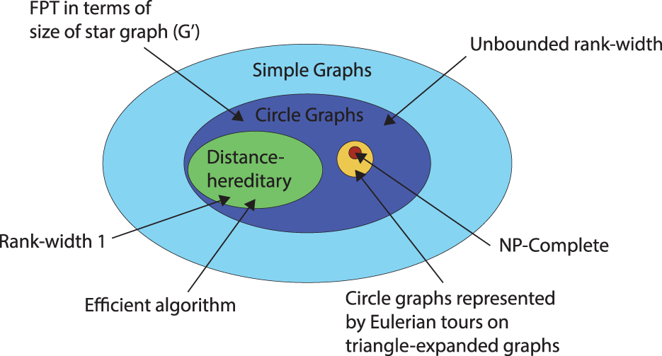
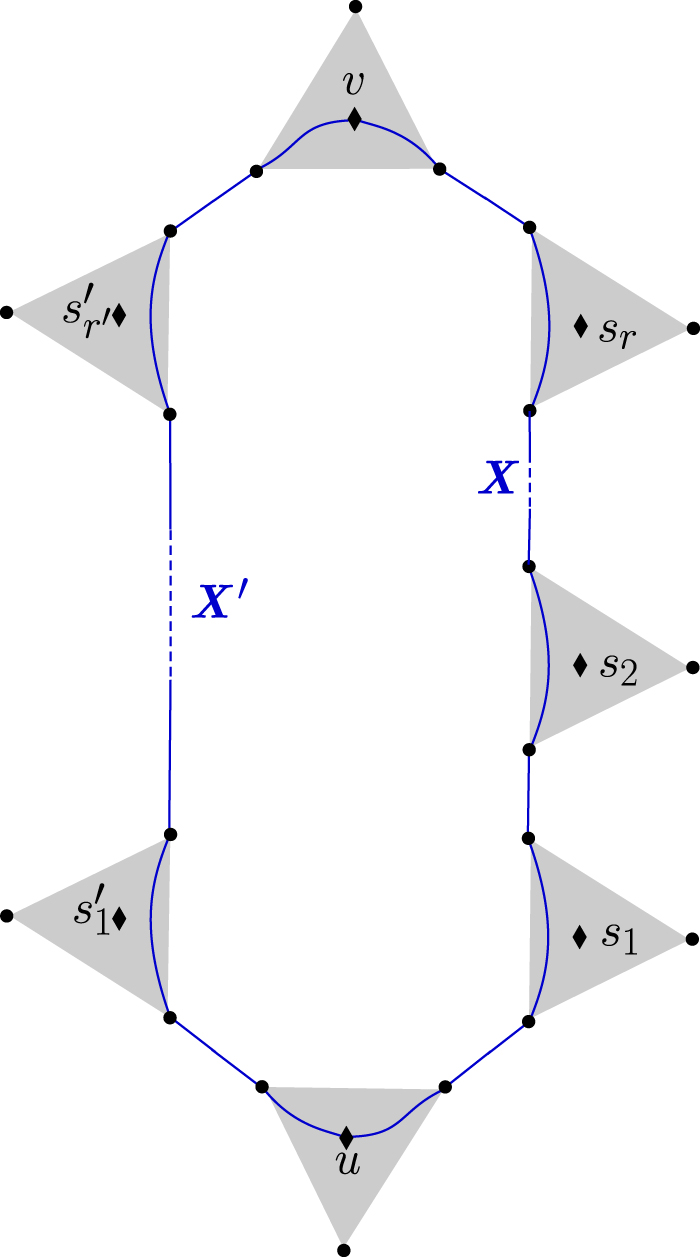
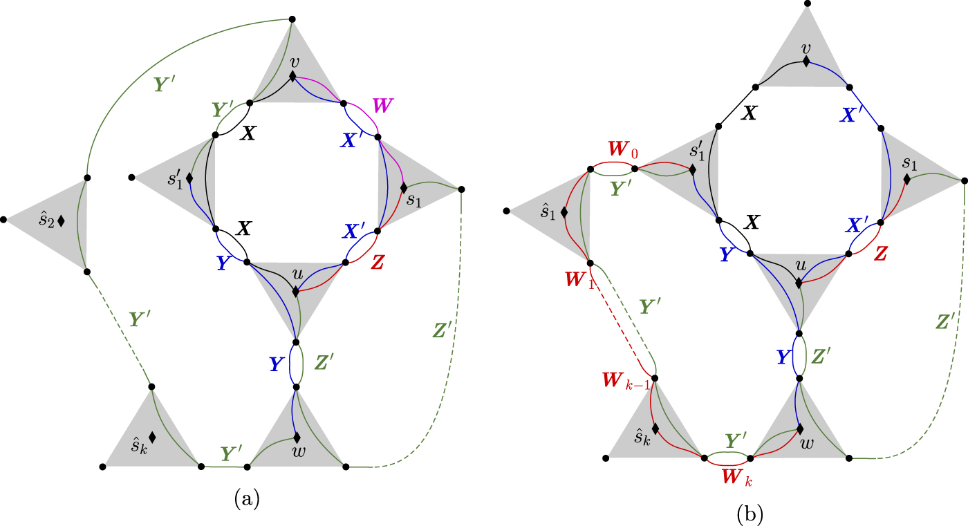
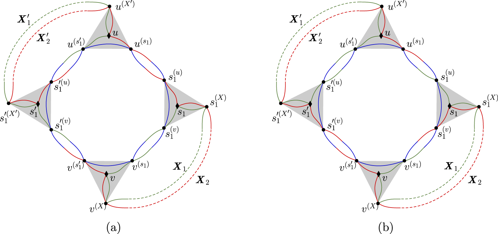