

Abstract
Background. Modern radiation therapy technologies aim to enhance radiation dose precision to the tumor and utilize hypofractionated treatment regimens. Verifying the dose distributions associated with these advanced radiation therapy treatments remains an active research area due to the complexity of delivery systems and the lack of suitable three-dimensional dosimetry tools. Gel dosimeters are a potential tool for measuring these complex dose distributions. A prototype tabletop solid-tank fan-beam optical CT scanner for readout of gel dosimeters was recently developed. This scanner does not have a straight raypath from source to detector, thus images cannot be reconstructed using filtered backprojection (FBP) and iterative techniques are required. Purpose. To compare a subset of the top performing algorithms in terms of image quality and quantitatively determine the optimal algorithm while accounting for refraction within the optical CT system. The following algorithms were compared: Landweber, superiorized Landweber with the fast gradient projection perturbation routine (S-LAND-FGP), the fast iterative shrinkage/thresholding algorithm with total variation penalty term (FISTA-TV), a monotone version of FISTA-TV (MFISTA-TV), superiorized conjugate gradient with the nonascending perturbation routine (S-CG-NA), superiorized conjugate gradient with the fast gradient projection perturbation routine (S-CG-FGP), superiorized conjugate gradient with with two iterations of CG performed on the current iterate and the nonascending perturbation routine (S-CG-2-NA). Methods. A ray tracing simulator was developed to track the path of light rays as they traverse the different mediums of the optical CT scanner. Two clinical phantoms and several synthetic phantoms were produced and used to evaluate the reconstruction techniques under known conditions. Reconstructed images were analyzed in terms of spatial resolution, signal-to-noise ratio (SNR), contrast-to-noise ratio (CNR), signal non-uniformity (SNU), mean relative difference (MRD) and reconstruction time. We developed an image quality based method to find the optimal stopping iteration window for each algorithm. Imaging data from the prototype optical CT scanner was reconstructed and analysed to determine the optimal algorithm for this application. Results. The optimal algorithms found through the quantitative scoring metric were FISTA-TV and S-CG-2-NA. MFISTA-TV was found to behave almost identically to FISTA-TV however MFISTA-TV was unable to resolve some of the synthetic phantoms. S-CG-NA showed extreme fluctuations in the SNR and CNR values. S-CG-FGP had large fluctuations in the SNR and CNR values and the algorithm has less noise reduction than FISTA-TV and worse spatial resolution than S-CG-2-NA. S-LAND-FGP had many of the same characteristics as FISTA-TV; high noise reduction and stability from over iterating. However, S-LAND-FGP has worse SNR, CNR and SNU values as well as longer reconstruction time. S-CG-2-NA has superior spatial resolution to all algorithms while still maintaining good noise reduction and is uniquely stable from over iterating. Conclusions. Both optimal algorithms (FISTA-TV and S-CG-2-NA) are stable from over iterating and have excellent edge detection with ESF MTF 50% values of 1.266 mm−1 and 0.992 mm−1. FISTA-TV had the greatest noise reduction with SNR, CNR and SNU values of 424, 434 and 0.91 × 10⁻⁴, respectively. However, low spatial resolution makes FISTA-TV only viable for large field dosimetry. S-CG-2-NA has better spatial resolution than FISTA-TV with PSF and LSF MTF 50% values of 1.581 mm−1 and 0.738 mm−1, but less noise reduction. S-CG-2-NA still maintains good SNR, CNR, and SNU values of 168, 158 and 1.13 × 10⁻⁴, respectively. Thus, S-CG-2-NA is a well rounded reconstruction algorithm that would be the preferable choice for small field dosimetry.
Export citation and abstract BibTeX RIS

Original content from this work may be used under the terms of the Creative Commons Attribution 4.0 licence. Any further distribution of this work must maintain attribution to the author(s) and the title of the work, journal citation and DOI.
1. Introduction
Radiation therapy is a crucial aspect of cancer treatment, with around 50% of cancer patients undergoing some form of radiotherapy during the course of their treatment [1, 2]. Advancements in radiation therapy technologies aim to personalize treatment plans, enhance radiation dose precision to the tumor, and utilize hypofractionated treatment regimens. These advancements include techniques like intensity-modulated radiotherapy (IMRT), volume modulated arc therapy (VMAT), stereotactic ablative radiotherapy and radiosurgery (SABR and SRS), and advanced imaging for daily target tracking and treatment adaptation. However, verifying the dose distributions associated with these advanced radiation therapy treatments remains an active research area due to the complexity of delivery systems and the lack of suitable three-dimensional dosimetry tools [3–6]. This comprehensive verification of dose distributions is of particular importance in SABR and SRS since treatments are delivered in five or fewer fractions with high conformation and rapid fall-off doses, hence a single geometric miss can result in a 20% or more dosimetric error [7]. Thus, there is a clear need for a robust and accurate 3D dosimetric system.
Advanced dose distributions implement complex 3D shapes with steep dose gradients that are challenging to measure using traditional dosimeters because of the restriction to point or planar measurements [5]. Gel dosimeters poise a potential tool in the measurement of complex dose distributions and can measure dose in a full 3D geometry while being nearly tissue equivalent. A unique characteristic of gel dosimeters is that the gel volume is both the phantom and the detector, which enables the verification of 3D dose distributions conveniently in a single measurement [8]. Gel dosimeters respond to radiation on the molecular level, thus the spatial resolution of the radiation induced response is limited only by the evaluation technique [9]. Due to the use of small fields (≤ 3 cm×3 cm) [10] and complex dose distributions, a spatial resolution of 1mm or better is required to resolve the dose distribution in steep gradient and fall-off regions [7, 11–14]. Cylindrical gel dosimeter inserts for head phantoms have been shown to be acceptable for the dose verification of clinical IMRT treatments [15, 16]. Gel dosimeters have also been used to determine the radiation isocenter of external beam treatment units [17].
Radiochromic gel dosimeters are designed specifically for imaging with optical computed tomography (CT) and elicit a colour change dose response, and hence an optical density change proportional to dose. Thus, the system measures dose by calculating the attenuation coefficients (contrast within the image) which is calibrated to dose for the specific gel formulation. Radiochromic gels, in general, have a number of attractive features and potential advantages over other gel dosimeters. Radiochromic gels can be manufactured in an open air environment with non-toxic materials and they absorb rather than scatter light, which facilitates high accuracy readout by optical CT [18]. Furthermore, radiochromic dosimeters possess high dose sensitivity that can be adjusted by changing the proportions of the dye and initiating agent [19].
Of the three primary imaging modalities for gel dosimetry, optical CT operates on similar principles as x-ray CT but offers distinct advantages for 3D dosimetry, particularly around potentially achieving higher accuracy and precision in shorter imaging times [3]. However, optical wavelength radiation experiences refraction when passing through different mediums in the optical CT system. Traditional filtered backprojection (FBP) image reconstruction assumes a straight raypath from source to detector thus, most optical CT scanners utilize a bath of refractive index matched fluid in which the dosimeter can be submerged to negate the effects of refraction allowing for reconstruction with FBP [20–27]. Although this method has led to good results (spatial resolution <1 mm) [24, 28], there are a number of issues with using a large volume of refractive index matched fluid. Often a mixture of several fluids is used and obtaining the excellent correspondence required between the refractive indices of the fluid and dosimeter can be very time consuming. Swirls of mismatching refractive indices can occur necessitating a careful balance between mixing and allowing the solution to settle. Furthermore, evaporation of the liquid must be accounted for. Finally, large volumes of refractive index matching fluid also limit the rotation speed due to the motion of the liquid [29] and are prone to dust and other airborne contamination [29, 30]. These issues have limited the clinical practicality of gel dosimeters.
A prototype tabletop solid-tank fan-beam optical CT scanner was developed by Ogilvy et al [31] with the intent to minimize the volume of refractive index matched fluid required by the system and thus remove the difficulties associated with a large volume of refractive index matched fluid. This scanner no longer relies on the assumption of a straight raypath from source to detector which, as a result, renders filtered backprojection (FBP) reconstruction unsuitable. Instead, iterative image reconstruction methods are employed to account for the refraction within the optical CT scanner.
Iterative image reconstruction algorithms can have a variety of iteration methods and objective functions [32–40]. A few of the most notable classes of techniques are algebraic reconstruction techniques (ART) and simultaneous iterative reconstruction techniques (SIRT). ART algorithms are row-action methods that treat the equations one at a time during the iterations, hence the ART methods are termed fully sequential. In contrast, SIRT algorithms use all the equations at the same time in one iteration, hence being termed simultaneous. Guenter et al [41] evaluated a collection 21 SIRT algorithms in terms of solution error, total variation and run time. The analysis was intended to compare a large number of algorithms on a large number of test problems with varying image properties and noise levels to determine the top-performing algorithms. Specifically, the novel work compares algorithms of two types: superiorization and regularization. A subset of 6 top performing algorithms in terms of solution error, total variation and run time were found. However, the system assumed a straight raypath from source to detector and did not account for refraction within the optical CT system. Furthermore, only solution error and total variation were considered in the image quality analysis. Here we further study this subset of top performing algorithms in terms of spatial resolution, signal-to-noise ratio (SNR), contrast-to-noise ratio (CNR), signal non-uniformity (SNU) and mean relative difference (MRD). These measures are utilized to quantitatively determine the optimal algorithm in terms of image quality while accounting for refraction within the optical CT system. Furthermore, we develop an image quality based method to find the optimal stopping iteration window for each algorithm. Lastly, imaging data from the prototype optical CT scanner is reconstructed and analysed to determine the optimal algorithm for this application.
2. Background
Iterative reconstruction algorithms are employed to solve large linear systems in tomography, represented by the general form equation

The reconstruction problem can be formulated by directly applying this linear equation to the Beer–Lambert law.
Applying the Beer–Lambert law to a single pixel, where Io is the initial light intensity and I is the collected intensity after leaving the medium, x can be written as the length of the ith ray through the jth pixel, xij . Likewise, μ can be written as the linear attenuation coefficient of the jth pixel calculated from the ith ray. Now summing over the entire system we have

Equation (2) can be rearrange into a linear equation of the form Ax = b,

and thus can be solved with iterative reconstruction algorithms. Rewriting equation (3) in the form of equation (1) we have, A = ∑i
∑j
xij
,  , and x = ∑i
∑j
μij
. We refer to A as the system matrix , b as the collected imaging data (sinogram) and x as the reconstructed image data. The system matrix, A, is constructed by discretizing the reconstruction region of the CT system into an N × N Cartesian grid, assuming linear ray traversal through each pixel. The matrix elements, aij
represent the weight coefficients that signify the contribution of the ith ray to the jth pixel. For a detector, the signal is treated as a single ray (or line) connecting the center of the detector element to the source. Therefore, the length of each ray passing through each pixel is calculated and compiled into the system matrix as the weight coefficients, aij
.
, and x = ∑i
∑j
μij
. We refer to A as the system matrix , b as the collected imaging data (sinogram) and x as the reconstructed image data. The system matrix, A, is constructed by discretizing the reconstruction region of the CT system into an N × N Cartesian grid, assuming linear ray traversal through each pixel. The matrix elements, aij
represent the weight coefficients that signify the contribution of the ith ray to the jth pixel. For a detector, the signal is treated as a single ray (or line) connecting the center of the detector element to the source. Therefore, the length of each ray passing through each pixel is calculated and compiled into the system matrix as the weight coefficients, aij
.
Solving equation (1) for large linear systems used in tomography is typically done by setting up a least-squares problem,

That is, by varying x such that the Euclidean norm of Ax − b is minimized gives the solution x⋆. Equation (1) can be solved directly using the normal equation AT Ax = AT b. However, this approach requires a full-rank matrix ATA, which is rare in tomography due to the sparsity and size of A. Direct solutions also tend to overfit the noise in the data, resulting in poor image quality. Therefore, iterative reconstruction algorithms are preferred for their ability to handle refraction and address these limitations.
The work of Guenter et al [41] analyzed three categories of iterative algorithms: base, superiorized, and regularized. Each category takes a different approach to finding the indirect solution to tomography problems.
Two base algorithms were investigated; the first known as Landweber [32] iteratively solves equation (1) and has form,

where λK is the relaxation parameter. The second base algorithm investigated was the conjugate gradient (CG) method. The CG method iteratively solves the normal equation AT Ax = AT b and the iterates have form xk+1 = xk + αk ρk , where αk is the current step size and ρk is the search direction (all search directions are cojugate vectors with respect to AT A).
Superiorized algorithms perturb the current iterate to a solution that is superior. This is done by taking a base algorithm and adding a perturbation step with one of the two utilized perturbation routines; nonascending direction (NA) [42] or fast gradient projection (FGP) [43]. Superiorization, in general, aims to improve the current solution at each iteration by revising it to meet a predefined secondary criterion.
Regularized algorithms solve the regularized least squares problem where a penalty term is added to equation (4),

where R(x) is the penalty term and λ is the regularization parameter that weights the importance of the penalty term.
3. Materials and methods
3.1. Optical CT scanner
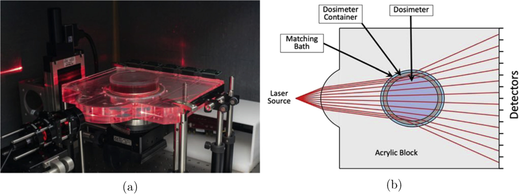
The protoype optical CT scanner is comprised of an acrylic (PMMA) block with a curved face and a 103.6 mm diameter bore hole in which the cylindrical radiochromic gel dosimeter is housed (figure 1). The dosimeter container has an outer diameter of 101.6 mm leaving a 2 mm gap between the container edge and bore hole. Thus, only a very small volume (10-35 ml) of refractive index matched fluid is required to fill the gap. While the fan-beam laser source and photodiode detector bay remain fixed, the dosimeter is rotated within the bore hole to acquire projections.

Figure 1. Optical CT scanner. (a) Image of the prototype tabletop solid-tank fan-beam optical CT scanner developed by Ogilvy et al [31] (b) Illustration of the optical CT scanner depicting the geometry and interfaces of the system.
Download figure:
Standard image High-resolution imageUtilizing the refraction at each interface, the geometry of the optical CT scanner has been optimized to achieve maximum light collection across the detector array, maximum volume of the dosimeter scanned, and maximum collected signal dynamic range [31]. The scanner has been designed for the use of the Flexydos3D dosimeter [44].
3.1.1. Clinical optical CT data
Using the prototype tabletop solid-tank fan-beam optical CT scanner, two clinical phantoms were imaged. The first phantom, dubbed the Circle and Square phantom, consists of a gel dosimeter with the active ingredient removed. This formulation of the gel has the same optical properties of the traditional formulation but with little to no attenuation. Both a circular column and a square column were molded into the gel using precisely measured inserts. The molds were then back-filled with a dyed gel formulation to give two regions of high attenuation. The circle has a diameter of 25.56 mm and the square has a length of 12.78 mm. The second phantom, dubbed the Needle phantom, consists of a set of 1.214 mm diameter (18 gauge) metal needles arranged in a grid pattern and cured into a gel dosimeter with the active ingredient removed.
3.1.2. Optical CT scanner noise characterization
The noise inherent within the prototype optical CT scanner was characterized by analyzing the initial light transmission data (Io ). Specifically, the standard deviation of each individual detector element (SDi ) was calculated from the normalized initial light transmission data. Normalization was achieved by subtracting the mean then dividing by the maximum, which yields a Gaussian distribution centered on zero with standard deviation representing the relative variability in light transmission. The average standard deviation over all detectors (SDave ) was then determined to give a quantitative metric of the inherent noise within the optical CT scanner.
3.2. Ray tracing simulator and system matrix generation
To track the light path through the different mediums of the prototype tabletop solid-tank fan-beam optical CT scanner, an in-house ray tracing simulator has been developed [31]. By discreziting the fan-beam laser source into rays, each ray is traced through the optical CT system while accounting for refraction (via Snell's law) at each interface and updating its trajectory. The system matrix, A, is a m × n matrix where m is the number of rays/detector elements (a single ray is traced to the center of each detector element), r, times the number of projections, θ, thus m = r · θ. 1280 rays/detector elements and 360 projections were used. Discretizing the reconstruction area of the optical CT scanner into an 512 × 512 Cartesian pixel grid produces a pixel size of 0.186mm/px. The system matrix elements, aij , are the length of the ith ray through the jth pixel. The length of each ray through each pixel was calculated by applying Siddon's algorithm [45] to the ray tracing simulator.
3.3. Synthetic optical CT data
Synthetic detector data (sinograms) replicating the data collection of the actual optical CT system was generated using our in-house ray tracing simulation. These synthetic sinograms were utilized to evaluate the iteratively reconstructed images under known conditions. At the interfaces of the optical CT system rays are both partially refracted and partially reflected. The total transmittance defines the ratio of refracted intensity to incident intensity and is calculated via the Fresnel equations.
Sinograms of simulated detector data were produced by generating synthetic phantoms with a variety of known attenuation distributions. Utilizing Siddon's algorithm [45], the length of each ray through each pixel was calculated and the resulting change in ray intensity due to the pixels attenuation was calculated using the Beer–Lambert law. The final intensity of each ray as it reaches a detector was calculated by summing over all traversed pixels. A simulated detector element measurement was then given by summing over all rays that reach a given detector. Applying this to all detector elements, over all the projection angles while accounting for both the partial transmitted intensity at interfaces and the attenuation through the synthetic phantom, a synthetic sinogram was calculated. Gaussian distributed noise is added to the synthetic sinograms. Each detector element at each projection had noise added (or subtracted) based on a single random sampling of the Gaussian probability distribution.
3.4. Iterative reconstruction
3.4.1. Image reconstruction
For input into the reconstruction algorithms the sinograms were reshaped from a matrix to a vector. A non-negativity constraint was applied to the algorithms as it is known a priori that the reconstruction should be strictly positive as negative linear attenuation coefficients (μ) are unphysical. For image display the reconstructed image data was reshaped from a vector to a N × N matrix.
3.4.2. Reconstruction algorithms
The reconstruction algorithms that were investigated were the top 6 performing algorithms set forth by Guenter et al [41] with the addition of the Landweber[32] algorithm to be used as a baseline for comparison. These algorithms are summarized in table 1. Of the top 6 performing algorithms, two were regularized algorithms: the fast iterative shrinkage/thresholding algorithm with total variation penalty term (FISTA-TV) and a monotone version of FISTA-TV (MFISTA-TV). Three superiorized CG methods were among the top performing algorithms: superiorized conjugate gradient with the nonascending perturbation routine (S-CG-NA), superiorized conjugate gradient with the fast gradient projection perturbation routine (S-CG-FGP) and superiorized conjugate gradient with with two iterations of CG performed on the current iterate and the nonascending perturbation routine (S-CG-2-NA). Finally, the last top performing algorithm was the superiorized Landweber algorithm with the fast gradient projection perturbation routine (S-LAND-FGP). All algorithms and algorithm parameters used were taken directly from the work of Guenter et al [41]. All algorithm parameters have been analyzed and tuned in previous work [41–43, 46, 47] to give the smallest errors on a variety of images.
Table 1. Investigated reconstruction algorithms.
| Class | Algorithm | Perturbation routine or penalty term | Abbreviation |
|---|---|---|---|
| Regularized | Fast iterative | ||
| shrinkage/thresholding | Total Variation | FISTA-TV | |
| Monotone fast iterative | |||
| shrinkage/thresholding | Total Variation | MFISTA-TV | |
| Superiorized | Conjugate Gradient | Nonascending | S-CG-NA |
| Conjugate Gradient | Fast Gradient Projection | S-CG-FGP | |
| Conjugate Gradient with two | |||
| iterations of CG performed | Nonascending | S-CG-2-NA | |
| on the current iterate | |||
| Landweber | Fast Gradient Projection | S-LAND-FGP | |
| Base | Landweber | N/A | Landweber |
3.5. Image quality analysis
A comprehensive evaluation of various image quality parameters was conducted for each iteration. To quantify spatial resolution, the modulation transfer function (MTF) was utilized, and three different methods were employed: point spread function (PSF), line spread function (LSF), and edge spread function (ESF) analyses. For PSF-based MTF calculation, a synthetic phantom with a single attenuating pixel was used, while the MTF based on LSF and ESF was determined using synthetic phantoms with a one-pixel-wide line of attenuating pixels and an edge between highly and non-attenuating regions, respectively.
Furthermore, the contrast-to-noise ratio (CNR) and signal-to-noise ratio (SNR) were computed for both synthetic and clinical images. Synthetic phantoms with a small, off-center circle of high uniform attenuation against a low attenuating background were employed for CNR and SNR calculations. Additionally, the Circle and Square phantom data were used to calculate CNR and SNR for the reconstructed clinical images. This was accomplished by defining separate signal regions of interest (ROIs) within the circle and square and comparing them against a background region.
The signal non-uniformity (SNU) of synthetic images was measured using a phantom with an off-center circle of high uniform attenuation and a low attenuating background. To obtain SNU values, the circle of high uniform attenuation was divided into several (9) sub-ROIs, and their mean grayscale values were compared. The same approach was applied to the Circle and Square phantom data to compute SNU for the reconstructed clinical images.
The mean relative difference (MRD) was calculated by averaging the relative difference from the known phantom of each pixel within the reconstructed images.
3.6. Stopping condition
3.6.1. Residual method
The stopping condition set out by Guenter et al [41] utilizes the residual, b − Axk , at each iteration to determine if iterating should cease. Specifically,

where,  is one half the Euclidean norm squared of the residual, σ2 is the variance of the noise within the imaging data. The variance of the noise, σ2 is chosen such that,
  , where
  is the maximum value within the imaging data, b, and 0.05 represents 5% noise.
3.6.2. Image quality method
A stopping condition based on image quality was used, involving several parameters calculated at each iteration. These parameters included spatial resolution at 50% MTF using PSF, LSF, and ESF synthetic phantoms, along with SNR, CNR, and SNU using a synthetic phantom with off-center high-attenuation circle and low-attenuation background. Mean relative difference was also computed for both Three Phase and Shepp-Logan synthetic phantoms. In total, 8 image quality parameters and reconstruction time were considered to determine the optimal stopping iteration for each algorithm. Faster reconstruction time with fewer iterations was considered advantageous.
A scoring system was employed to determine the optimal stopping iteration for each algorithm. A weighting scheme (table 2) was used to define this quantitative metric for determining the optimal number of iterations. The weighting factors to determine optimal iteration number have been defined such that spatial resolution, noise, mean relative difference and time are of equal value to the overall score of the algorithm. This is to provide a quantitative metric that analyzes algorithms in terms of meeting the Resolution-Time-Accuracy-Precision (RTAP) criteria set forth by Oldhem et al [14] that describes the requirements for dosimetric verification of radiation therapy treatment plans. The final score was computed via the following equation,

In equation (8), base values are MTF50PSF
, MTF50LSF
, MTF50ESF
, SNR, CNR, SNU, MRD3Phase
, MRDSL
and iteration. The value  is taken as the maximum value over 300 iterations. The weights w⋯ are provided in table 2. Notice that for parameters where a minimum value is preferred (SNU, mean relative difference, and time), the score was subtracted from unity. From table 2, it is clear that the maximum total score achievable was 4 with each category of spatial resolution, noise reduction, mean relative difference, and time contributing a value of 1 to the total score. To produce a window of stopping iterations, spatial resolution was given higher weight in one case (spatial resolution importance: 1.75, noise reduction importance: 0.25) and higher weight for noise reduction in the other case (spatial resolution importance: 0.25, noise reduction importance: 1.75). The optimal stopping iteration was determined based on the number of iterations that received the highest score for each weighted case. These ancillary stopping iterations established a range for terminating the algorithms.
Table 2. Image quality stopping condition weighting. PSF/LSF/ESF at 50% MTF. S-L=Shepp-Logan.
| Optimal | Optimal | Noise | Noise | Resolution | Resolution | Clinical | Clinical | ||
|---|---|---|---|---|---|---|---|---|---|
| weight | total | weight | total | weight | total | weight | total | ||
| Spatial Resolution | PSF | 0.333 | 0.083 | 0.583 | 1 | ||||
| LSF | 0.333 | 1 | 0.083 | 0.25 | 0.583 | 1.75 | N/A | 1 | |
| ESF | 0.333 | 0.083 | 0.583 | N/A | |||||
| Noise | SNR | 0.333 | 0.583 | 0.083 | 0.333 | ||||
| CNR | 0.333 | 1 | 0.583 | 1.75 | 0.083 | 0.25 | 0.333 | 1 | |
| SNU | 0.333 | 0.583 | 0.083 | 0.333 | |||||
| MRD | 3 Phase | 0.5 | 0.5 | 0.5 | N/A | ||||
| S-L | 0.5 | 1 | 0.5 | 1 | 0.5 | 1 | N/A | N/A | |
| Time | 1 | 1 | 1 | 1 | 1 | 1 | 1 | 1 | |
| Total | 4 | 4 | 4 | 3 | |||||
3.7. Optimal algorithm determination
To determine the optimal algorithm, the image quality parameters at the stopping iterations were used in equation (8), however, they were now divided by the global maximum across all algorithms such that their score relative to all algorithms was calculated. The synthetic images were scored again according to table 2 with the images at the noise reduction stopping condition used for the noise reduction weighted scoring and, likewise, images at the spatial resolution stopping condition used for the spatial resolution weighted scoring. Clinical images were scored according to table 2 for all stopping iterations. Note that, SNR, CNR and SNU values for the clinical images are calculated twice, once from the circle of high attenuation and once from the square of high attenuation. Thus, the clinical weight of 0.333 for each parameter is split over the circle and square calculations yielding a weight of 0.1665.
4. Results 4
4.1. Optical CT scanner noise characterization
The prototype optical CT scanner was found to have Gaussian distributed noise with an average initial transmission standard deviation of SDave = 0.0455 (4.55%). Figure 2 shows a distribution of initial transmission collection data (Io ) for detector element number 75. This value encompasses all types and sources of noise within the scanning system (manufacturing imperfections, electronic noise, etc.) as it is calculated from the initial transmission data (Io ). Therefore, synthetic image quality analysis performed with 5% Gaussian noise added to the synthetic data is deemed a reasonable and accurate representation of the physical optical CT system.

Figure 2. Exemplary distribution of the normalized initial transmission collection data (Io ) for detector element number 75.
Download figure:
Standard image High-resolution image4.2. Residual method stopping condition
The residual method stopping condition is shown in figure 3(a) as a horizontal line that when crossed terminates the iterative process. This method is not robust as several algorithms never reach the stopping condition while others are stopped prematurely. The magnitude of the residual value at plateau is also dependent on the phantom (attenuation distribution). In other words, using the residual as a stopping condition can be inconsistent as the magnitude of the residual is image and algorithm dependent. Furthermore, this stopping condition exhibits its constraint on the number of iterations purely based on the magnitude of the residual. However, it is shown in figure 3(b) that the minimizing of the residual does not always increase the resultant image quality. After a certain number of iterations, the image can become over-iterated, leading to a noise-dominated image despite decreasing residual magnitudes. This phenomenon, known as 'semi-convergent behavior', is evident in figure 3(b). The mean relative difference increases away from the minimum, while SNR values initially reach a maximum but then decline due to over-iteration introducing noise. Spatial resolution may still increase to a maximum in some cases, but not universally for all iterative algorithms. This disconnect between the magnitude of the residual and the resultant image quality is remedied by the image quality based stopping condition presented in the following section.

Figure 3. (a) Residual values for all reconstruction algorithms as a function of iterations for the Three Phase phantom. The residual method stopping condition is shown as a horizontal line that when crossed terminates the iterative process. (b) Image quality parameter values for the Landweber reconstruction algorithm as a function of iterations. The residual method stopping iteration is shown as a vertical line.
Download figure:
Standard image High-resolution image4.3. Iterative algorithm behaviour and image quality method stopping condition
Each iterative reconstruction algorithm was analyzed (as described in section 3.5) using synthetic optical CT data both without and with 5% Gaussian noise added. The noiseless analysis aimed to characterize the general behavior of each algorithm as iterations increased. Gaussian noise of 5% was added to the synthetic data such that the algorithm specific stopping condition could be determined under known conditions that mimic the actual imaging data from the prototype optical CT scanner. This allows for analysis where the phantom is known a priori and reconstructed images can be directly compared. The algorithm specific stopping condition can then be directly applied to actual imaging data from the prototype optical CT scanner. Each algorithm specific stopping condition is described in table 3. Any changes to the general behaviour of the algorithm due to the introduction of noise in the imaging data is described in the following sections. In figures 4–9, dots represent the critical values, with red dots representing the maximum value for parameters where the maximum is advantageous (spatial resolution, SNR and CNR) and blue dots representing the minimum value where minimum is advantageous (SNU and MRD). Vertical lines represent the recommended algorithm specific stopping condition with the thick vertical line indicating the optimal iteration.

Figure 4. Landweber image quality parameters as a function of iterations. (a) 0% noise (b) 5% Gaussian noise.
Download figure:
Standard image High-resolution imageTable 3. Algorithm specific image quality based stopping condition.
| Algorithm | Optimal | Resolution weighted | Noise weighted |
|---|---|---|---|
| Landweber | 20 | 39 | 18 |
| FISTA-TV | 59 | 54 | 59 |
| MFISTA-TV | 67 | 48 | 67 |
| S-CG-NA | 67 | 54 | 67 |
| S-CG-FGP | 46 | 46 | 46 |
| S-CG-2-NA | 62 | 91 | 54 |
| S-LAND-FGP | 118 | 142 | 85 |
4.3.1. Landweber
Figure 4 shows the image quality results of the Landweber algorithm. Examining figure 4, we see the spatial resolution (50% MTF) gradually increases to a maximum and then plateaus for all spatial resolution calculation methods (PSF, LSF, and ESF). SNR and CNR values initially rise to their maximum, but later decrease due to introduced noise during over-iteration. SNU exhibits a slight increase followed by a sharp decline and stabilization at a minimum. The mean relative difference from known phantoms sharply decreases with oscillations, reaching a minimum. However, over-iteration causes a gradual increase in the mean relative difference, amplifying image noise. These typical iterative image reconstruction characteristics involve increasing spatial resolution and decreasing noise until over-iteration.
With 5% Gaussian noise added to the synthetic data, spatial resolution (50% MTF) for PSF and LSF increases gradually but slower than the noiseless analysis. The ESF-based spatial resolution exhibits a distinct pattern: a quick increase to maximum, a short plateau, and a rapid decrease due to high noise affecting edge resolution. SNR, CNR, and SNU follow similar trends as in the noiseless analysis but with earlier attainment of maximum/minimum values and sharper transitions. The mean relative difference also follows noiseless trends but with a faster increase after reaching the minimum value. These changes indicate that the effects of over-iteration are more significant with added noise.
The stopping iteration window ranges from 18 to 39 iterations, with the low end emphasizing noise reduction at the expense of spatial resolution, and the high end yielding the opposite outcome.
4.3.2. FISTA-TV
Figure 5 shows the image quality results of the FISTA-TV algorithm. Examining figure 5, we see the PSF and LSF-based spatial resolution remains constant throughout iterations, while the ESF-based spatial resolution rapidly increases in the first 50 iterations and then stabilizes. SNU shows a slight initial increase followed by a sharp decrease to a minimum value. SNR and CNR values increase to a maximum within the first 50 iterations, fluctuating slightly, and then plateau slightly below the maximum value with further iterations. The mean relative difference from known phantoms sharply decreases and remains slightly above the minimum value. FISTA-TV is characterized by its stability, as image quality parameters stay near their critical values once achieved, making the effects of over-iteration negligible.
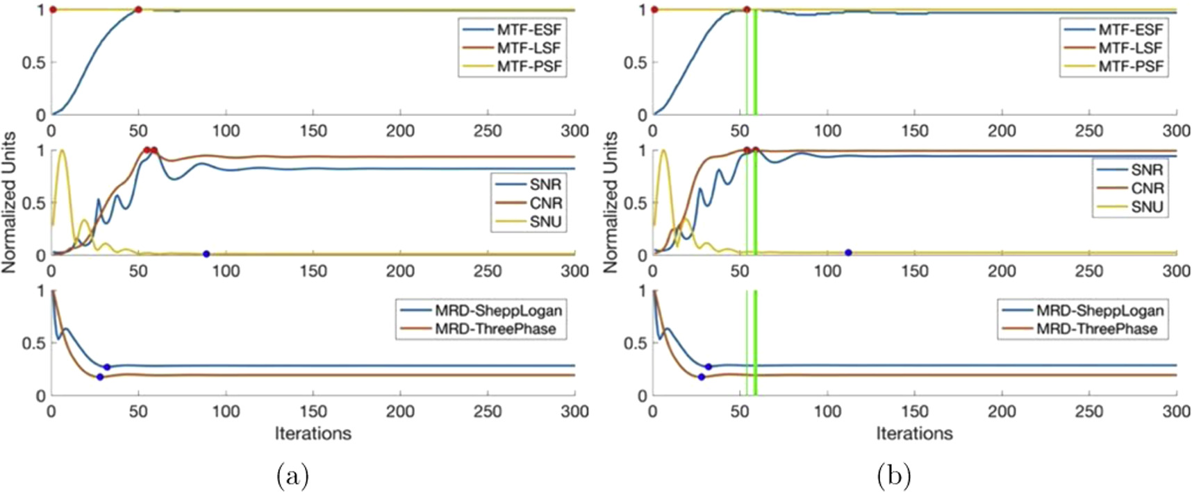
Figure 5. FISTA-TV image quality parameters as a function of iterations. (a) 0% noise (b) 5% Gaussian noise.
Download figure:
Standard image High-resolution imageAll image quality parameter characteristics remain unchanged with the introduction of 5% Gaussian noise, except for a slight decrease in ESF-based spatial resolution from the maximum, which then remains constant.
The stopping iteration window ranges from 54 to 59 iterations, with the lower end slightly favoring ESF spatial resolution due to the slight decrease before stabilization. However, given FISTA-TV's stability, any number of iterations beyond 54 will yield images with negligible differences in quality. Hence, the stopping iteration can be viewed as a minimum rather than a window of iterations.
4.3.3. MFISTA-TV
MFISTA-TVs attributes are nearly identical to FISTA-TV (as expected) as they are nearly identical algorithms (figure A1 in appendix). However, MFISTA-TV was unable to resolve both the PSF and LSF displaying a blank image at every iteration. As such, the corresponding 50% MTF values are at a constant value of zero. Furthermore, the SNR and CNR values remain constant at maximum once reached, as opposed to slightly below the maximum. With the inability to resolve the PSF and LSF, MFISTA-TV is deemed unsuitable to be an effect reconstruction technique for small field dosimetry and will be disregarded from further analysis.
4.3.4. S-CG-NA
Figure 6 shows that SNR and CNR values exhibit rapid random fluctuations throughout iterations, ranging between the maximum and one-tenth of the maximum. The introduction of noise produces SNU values that also exhibit rapid random fluctuations, as well as, exacerbating the fluctuations in SNR and CNR values. Although, the stopping iteration window ranges from 54 to 67 iterations, the major fluctuations in several metrics makes the window, and the algorithm in general, unreliable.
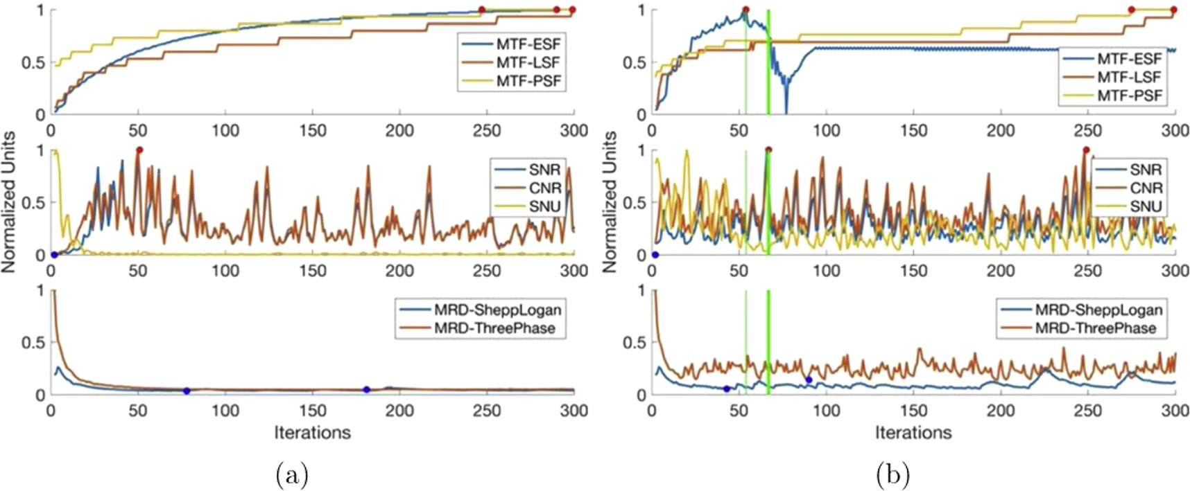
Figure 6. S-CG-NA image quality parameters as a function of iterations. (a) 0% noise (b) 5% Gaussian noise.
Download figure:
Standard image High-resolution image4.3.5. S-CG-FGP
Illustrated in figure 7, the stopping iteration for S-CG-FGP is at iteration 46, due to the large spike in SNR and CNR values. If this spike is ignored, the stopping iteration window would span from around 40 to 100 iterations, as all image quality parameters remain relatively constant within that interval. However, there is no stopping iteration window that encompasses both high spatial resolution and high noise reduction. Specifically, the LSF resolution increase and PSF resolution ceasing oscillation occurs only after the SNR and CNR values have started to plateau around zero.
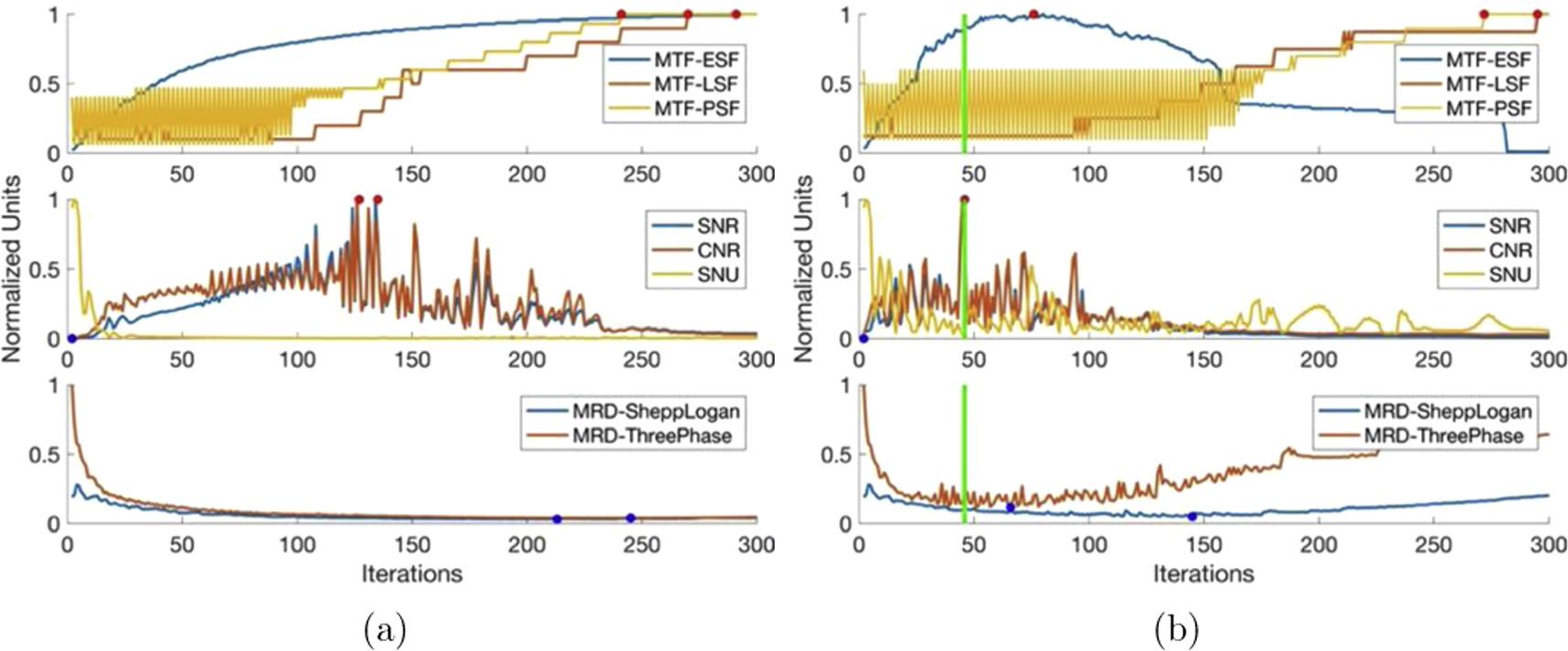
Figure 7. S-CG-FGP image quality parameters as a function of iterations. (a) 0% noise (b) 5% Gaussian noise.
Download figure:
Standard image High-resolution image4.3.6. S-CG-2-NA
Figure 8 shows the stopping iteration window ranges from 54 to 91 iterations for the S-CG-2-NA algorithm. Beyond 91 iterations, the large single-iteration oscillations of SNR and CNR cease, and the image quality parameters stabilize. Thus, considering iteration 91 as the minimum number of iterations avoids the large oscillations and deems the algorithm stable against over-iteration. However, this approach results in reduced CNR values compared to the optimal number of iterations and increased reconstruction time.
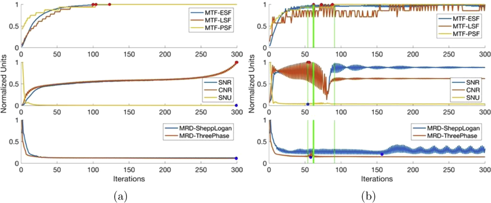
Figure 8. S-CG-2-NA image quality parameters as a function of iterations. (a) 0% noise (b) 5% Gaussian noise.
Download figure:
Standard image High-resolution image4.3.7. S-LAND-FGP
Figure 9 shows the stopping iteration window for S-LAND-FGP ranges from 85 to 142 iterations, based on the ESF MTF 50% value, as all other image quality parameters remain constant within that interval. Thus, the stopping iteration window represents a trade-off between reconstruction time and ESF spatial resolution, with the high end yielding higher ESF spatial resolution at the expense of longer reconstruction time, and vice versa for the low end.

Figure 9. S-LAND-FGP image quality parameters as a function of iterations. (a) 0% noise (b) 5% Gaussian noise.
Download figure:
Standard image High-resolution image4.4. Image quality analysis
4.4.1. Synthetic data
Figure 10 shows spider plots of the the image quality parameters calculated for each iterative algorithm from the synthetic imaging data with 5% Gaussian noise. Qualitatively, the spider plots can be interpreted with the larger the area encompassed by the parameter arms the better the performance of the algorithm. FISTA-TV had the highest score for both the optimal weighted scoring system as well as the noise reduction weighted scoring system. S-CG-2-NA had the highest spatial resolution weighted score. The specific parameter values can be found in table A1 of the appendix.

Figure 10. Synthetic image quality at stopping condition (a) Landweber (b) FISTA-TV (c) S-CG-NA (d) S-CG-FGP (e) S-CG-2-NA (f) S-LAND-FGP.
Download figure:
Standard image High-resolution image4.4.2. Clinical data
Figure 11 shows spider plots of the the image quality parameters calculated for each iterative algorithm from the clinical imaging data. FISTA-TV had the highest score for all three of the; optimal, spatial resolution and noise reduction weighted scoring systems. The specific parameter values can be found in table A2 of the appendix.
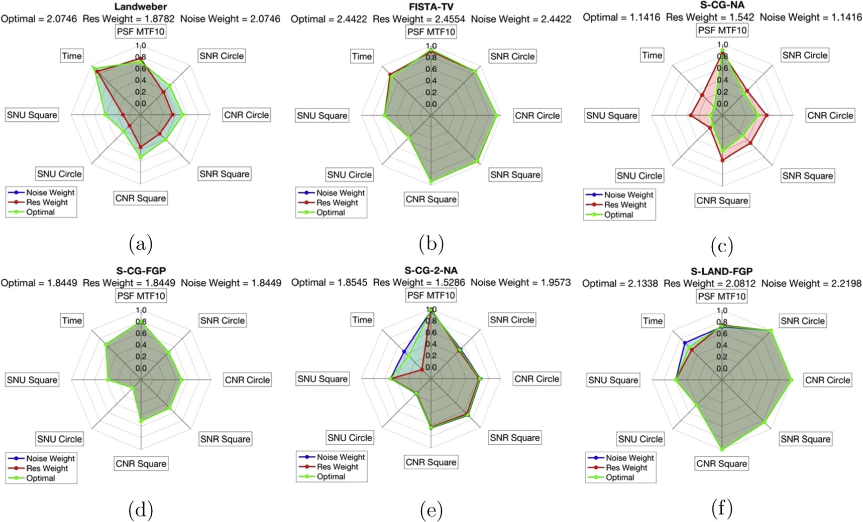
Figure 11. Clinical Image quality at stopping condition (a) Landweber (b) FISTA-TV (c) S-CG-NA (d) S-CG-FGP (e) S-CG-2-NA (f) S-LAND-FGP.
Download figure:
Standard image High-resolution image4.5. Optimal algorithms
The algorithms in which received the highest score for at least one of the weighted scoring systems were FISTA-TV and S-CG-2-NA. These two algorithms are qualitatively compared to FBP and the known image in figure 12 to demonstrate the increased image quality iterative methods achieve over traditional methods. It is evident that that FBP produces an extremely distorted image, and thus inaccurate dosimetric information, due to refraction not being accounted for.
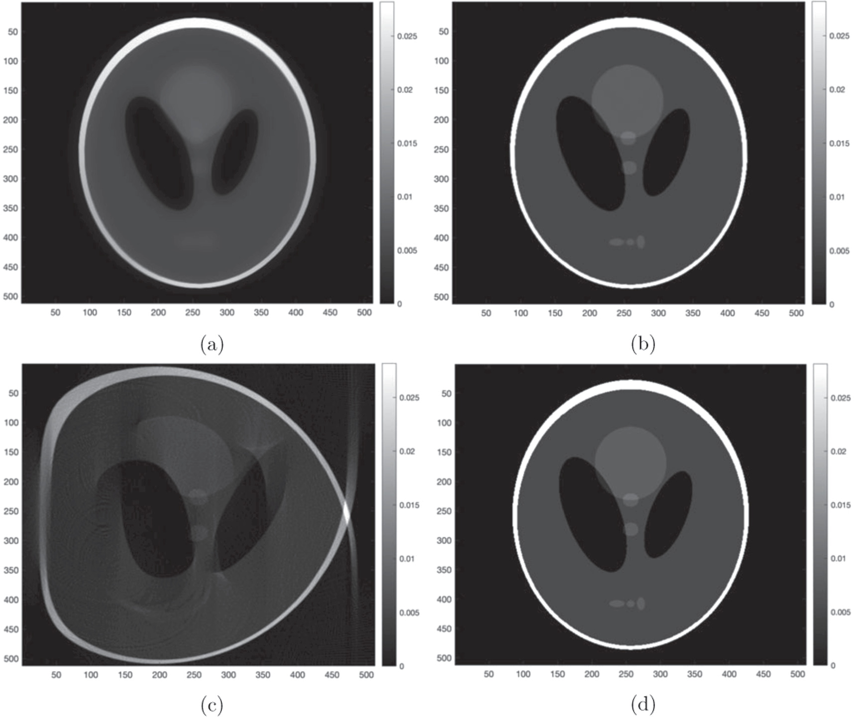
Figure 12. Shepp-Logan synthetic phantom with 0% noise reconstructed with: (a) FISTA-TV, (b) S-CG-2-NA and (c) FBP. (d) The known Shepp-Logan synthetic phantom.
Download figure:
Standard image High-resolution imageFISTA-TV and S-CG-2-NA were analyzed further to showcase their strengths and weaknesses as well as to provide insight into the application in which the algorithm will be most effective.
Figure 13(a) compares the performance of the FISTA-TV and S-CG-2-NA algorithms on the Three Phase synthetic phantom with 5% Gaussian noise. FISTA-TV produces an image with very little noise however, the high attenuation peaks are under valued. More specifically, the attenuating object at pixels 160-225 is reconstructed well by FISTA-TV, being only slightly undervalued due to the smoothing of noise. The objects at pixels 40-80 and 445-485 are smaller in size and the smoothing attributes of FISTA-TV begin to undervalue the object. Conversely, S-CG-2-NA produces an image with the high attenuation peaks more accurately resolved, however there is a larger amount of image noise.
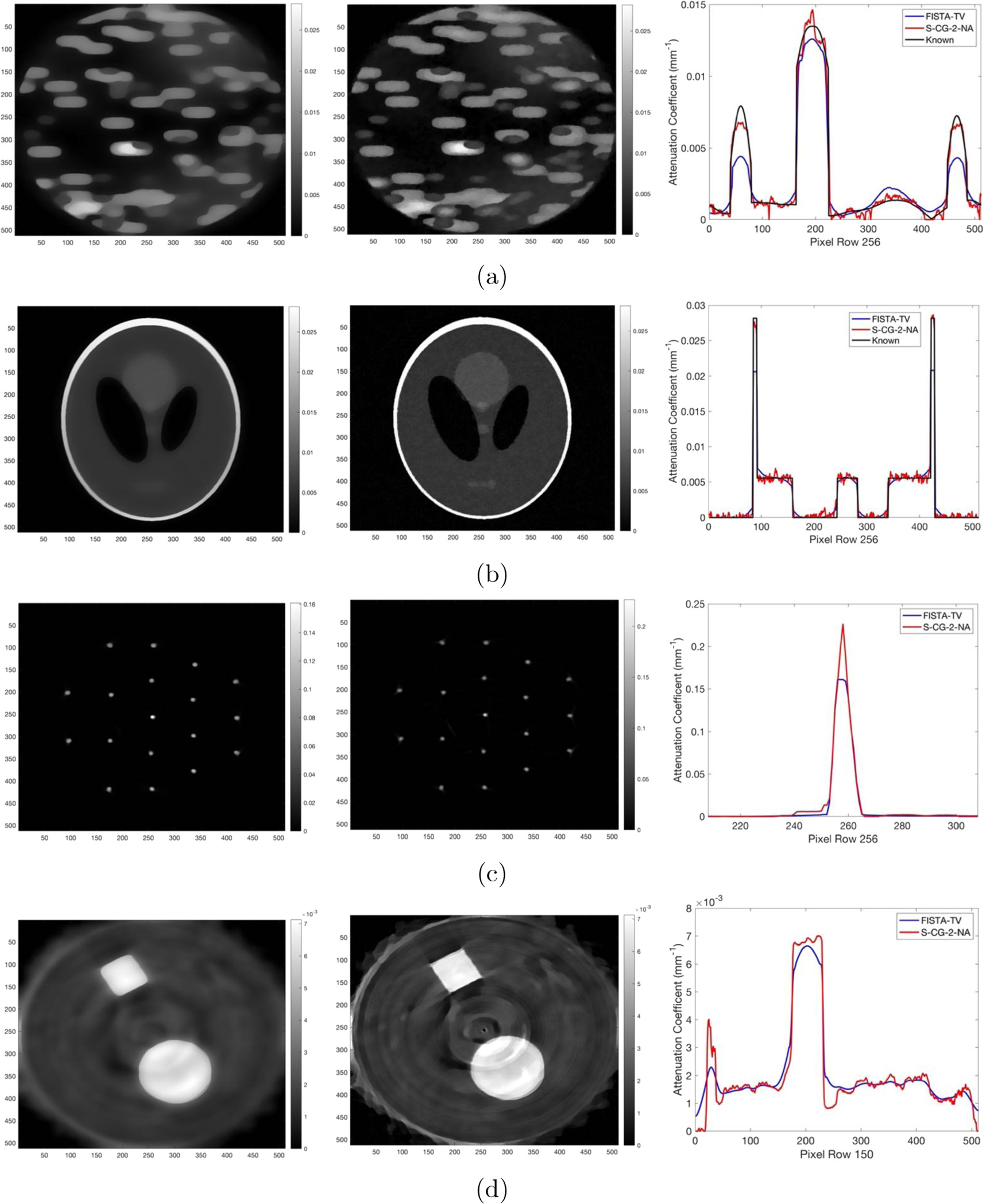
Figure 13. Images reconstructed with FISTA-TV (left), S-CG-2-NA (middle) and profiles taken through the center row (right). (a) Three Phase synthetic phantom with 5% Gaussian noise, (b) Shepp-Logan synthetic phantom with 5% Gaussian noise, (c) Needle clinical phantom, (d) Circle Square clinical phantom (Profiles taken through row 150).
Download figure:
Standard image High-resolution imageExamining figure 13(b), FISTA-TV reconstructs an image with very little noise showcasing its smoothing ability. However, the small structures within the Shepp-Logan phantom are not resolved. S-CG-2-NA reconstructs an image with much higher noise as seen by the graininess of the image but is able to resolve the small structures showcasing the algorithms superior spatial resolution.
Examining figure 13(c), we see that the effects of FISTA-TV's low spatial resolution are much less notable when considering the clinical imaging data from the prototype optical CT scanner. This is largely due to the needle having a diameter of 1.214 mm and thus large enough to be reconstructed with comparable accuracy to S-CG-2-NA.
In figure 13(d), it is shown that the effects of FISTA-TV's low spatial resolution are somewhat noticeable qualitatively, when considering the clinical imaging data, as the rounding of the corners of the square of high attenuation. S-CG-2-NA is able to reconstruct the corners more sharply, but again, at the cost of less noise reduction.
5. Discussion
The prototype optical CT scanner was found to have Gaussian distributed noise with an average standard deviation of 4.55%. This motivated the addition of 5% Gaussian noise to the synthetic CT data, such that, the synthetic data gives a reasonable and accurate representation of the physical optical CT system. This ensures the analysis of the synthetic data is generalizable to the clinical optical CT data.
The algorithms characterized as regularized model algorithms (FISTA-TV and MFISTA-TV) have stability from over iterating with high levels of smoothing, therefore high noise reduction but low spatial resolution. MFISTA-TV was found to behave almost identically to FISTA-TV however MFISTA-TV was unable to resolve the PSF and LSF synthetic phantoms. Superiorized conjugate gradient algorithms with the nonascending direction perturbation routine (S-CG-NA and S-CG-2-NA) have high spatial resolution and thus high noise. Superiorized conjugate gradient algorithm with the fast gradient projection perturbation routine (S-CG-FGP) conversely has low spatial resolution with high noise reduction, showcasing the importance of the perturbation routine on image quality. Landweber has extremely high noise, so much so that the ESF is unresolved after a number of iterations but has good spatial resolution otherwise. Once superiorized with the fast gradient projection perturbation routine the opposite is true; high noise reduction with low spatial resolution. Again, this reversal of behaviour showcases the large effect that the perturbation routine has on image quality. The algorithms that had higher smoothing and noise reduction performed better in term of spatial resolution for the ESF indicating that edges are still very well resolved but small structures succumb to the low spatial resolution. This makes these algorithms less optimal for small field dosimetry, but a viable option for large field (≥ 3 cm×3 cm) dosimetry in which edge resolution is of importance.
S-CG-NA showed extreme fluctuations in the SNR and CNR values at all iterations. This instability makes S-CG-NA undesirable to use as there is large quantitative differences when reconstruction is varied by just a single iteration. Like S-CG-NA, S-CG-FGP has large fluctuations in the SNR and CNR values and the algorithm has less noise reduction than FISTA-TV and worse spatial resolution than S-CG-2-NA. Therefore, S-CG-FGP can be disregarded. S-LAND-FGP has many of the same characteristics as FISTA-TV; high noise reduction and stability from over iterating. However, S-LAND-FGP has worse SNR, CNR and SNU values as well as a longer reconstruction time, so can be disregarded.
The optimal algorithms found through the quantitative scoring metric were FISTA-TV and S-CG-2-NA.Selection between these two algorithms is dependent on the specific needs of the user. In the scenario in which noise reduction is of higher importance or where smoothly varying data is present and edge detection is of higher importance than resolution of small structures, FISTA-TV is more advantageous. S-CG-2-NA is more advantageous to use when spatial resolution and resolution of small structures is of the highest importance.
FISTA-TV provides excellent edge detection represented by the high ESF MTF 50% of 1.266 mm−1 meaning it is capable of accurately measuring steep dose gradients. The algorithm is less effective at reconstructing a single attenuating pixel and a line of attenuating pixels one pixel wide, represented by the poor PSF and LSF MTF 50% values. However, these metrics are less clinically relevant as the system has a pixel size of 0.186 mm which is much smaller than even the most stringent tolerances. Comparing FISTA-TV to the ordered subsets convex algorithm with TV-regularization (OSC-TV) presented by Matenine et al [35], FISTA-TV produces greater spatial resolution. OSC-TV was found to have a MTF 52% of 1 mm−1 [36]. This value is obtained from an edge phantom and no analysis is done using a point or line phantom. The work of Dekker et al [48] also utilizes OSC-TV but does not present specific spatial resolution values, rather, a reduction in 95%-5% distance when compared to FBP. Qualitatively, the work shows sharp dose gradients on phantoms of various sizes. However, the smallest field size analyzed was 0.6cm x 0.6 cm. Effectively, this analysis again is looking at an ESF where FISTA-TV performs very well. The small structures within the Shepp-Logan phantom that are unresolved by FISTA-TV (figure 13(b)) are on the order of 3 mm in diameter and only have a slight attenuation difference from the background. These two compounding factors (smaller field size and low contrast difference) explain the inability of FISTA-TV to resolve those structures. Conversely, FISTA-TV is able to resolve the 1.214 mm diameter needles within the clinical needle phantom with sharp edges as they have a larger contrast difference from the background. The prototype optical CT scanner is prone to ring artifacts as seen in figure 13(d). These artifacts are due to issues with the current photodiode detector bay. While active work is being performed to implement a less problematic detector bay, ring artifacts are a common issue in optical CT that cannot be completely eliminated. FISTA-TV alleviates the prevalence of these artifacts through its smoothing behaviour and further points to an advantage of the algorithm.
S-CG-2-NA has superior spatial resolution to all algorithms while still maintaining good noise reduction. Furthermore, the algorithm is uniquely stable from over iterating where the other conjugate gradient algorithms with the nonascending direction perturbation are not. Comparing S-CG-2-NA to the simultaneous algebraic reconstruction technique integrated with ordered subsets iteration and total variation minimization regularization (SART+OS+TV) analyzed by Du et al [40], shows similar ability to resolve a needle phantom. Furthermore, S-CG-2-NA produces similar CNR values (17.6-19.4) compared to SART+OS+TV (8.9002-61.0379). However, the SART+OS+TV analysis is performed on data collected from an optical CT scanner that has straight raypath geometry.
6. Conclusion
The optimal algorithms found through the quantitative scoring metric were FISTA-TV and S-CG-2-NA. Both algorithms were stable from over iterating and had excellent edge detection with ESF MTF 50% values of 1.266 mm−1 and 0.992 mm−1, respectively. FISTA-TV had the greatest noise reduction with SNR, CNR and SNU values of 424 , 434 and 0.91 × 10⁻⁴, respectively. However, extremely low PSF and LSF MTF 50% values make FISTA-TV better suited for large field dosimetry, where noise reduction is of higher importance than spatial resolution. S-CG-2-NA had greater spatial resolution with PSF and LSF MTF 50% values of 1.581 mm−1 and 0.738 mm−1, respectively. The algorithms noise reduction is less than that of FISTA-TV but still maintained good SNR, CNR, and SNU values of 168, 158 and 1.13 × 10⁻⁴, respectively. S-CG-2-NA is thus a well rounded reconstruction algorithm that would be the preferable choice for small field dosimetry.
Data availability statement
The data that support the findings of this study are openly available at the following URL/DOI: https://osf.io/94yg5/.
Conflict of interest
The authors have no relevant conflicts of interest to disclose.
Appendix

Figure A1. MFISTA-TV image quality parameters as a function of iterations. Dots represent the critical values, with red dots representing the maximum value for parameters where the maximum is advantageous (spatial resolution, SNR and CNR) and blue dots representing the minimum value where minimum is advantageous (SNU and MRD). Vertical lines represent the recommended algorithm specific stopping condition with the think vertical line indicating the optimal iteration. (a) 0% noise (b) 5% Gaussian noise.
Download figure:
Standard image High-resolution image
Table A1. Image quality parameters for each iterative algorithm at the optimal stopping iteration from the synthetic imaging data with 5% Gaussian noise.
| Algorithm (Iterations) | ESF MTF50 [ mm−1] | LSF MTF50 [ mm−1] | PSF MTF50 [ mm−1] | SNR | CNR | SNU (×10−4) | MRD Shepp-Logan [%] | MRD Three Phase [%] | Time [s] |
|---|---|---|---|---|---|---|---|---|---|
| Landweber (20) | 0.287 | 0.527 | 0.843 | 39 | 45 | 3.66 | 7.03 | 42.69 | 28.2 |
| FISTA-TV (59) | 1.266 | 0.105 | 0.211 | 424 | 434 | 0.91 | 4.10 | 31.19 | 90.9 |
| MFISTA-TV (67) | 1.266 | 0 | 0 | 415 | 433 | 0.80 | 4.06 | 31.82 | 153.1 |
| S-CG-NA (67) | 0.718 | 0.949 | 1.265 | 102 | 78 | 1.86 | 3.27 | 32.74 | 468.7 |
| S-CG-FGP (46) | 1.083 | 0.105 | 0.105 | 228 | 197 | 2.01 | 3.94 | 25.96 | 115.0 |
| S-CG-2-NA (62) | 0.992 | 0.738 | 1.581 | 168 | 158 | 1.13 | 3.58 | 17.13 | 344.1 |
| S-LAND-FGP (118) | 1.148 | 0.105 | 0.211 | 289 | 411 | 1.04 | 5.65 | 43.13 | 199.1 |
Table A2. Image quality parameters for each iterative algorithm at the optimal stopping iteration from the clinical imaging data.
| Algorithm | PSF MTF10 [ mm−1] | Circle SNR | Square SNR | Circle CNR | Square CNR | Circle SNU (10−3) | Square SNU (10−3) |
|---|---|---|---|---|---|---|---|
| Landweber | 0.525 | 11.4 | 19.5 | 14.5 | 16.1 | 1.13 | 0.62 |
| FISTA-TV | 0.682 | 19.7 | 43.6 | 25.4 | 28.2 | 0.95 | 0.42 |
| MFISTA-TV | 0.682 | 20.3 | 47.8 | 25.6 | 28.1 | 0.92 | 0.40 |
| S-CG-NA | 0.661 | 7.3 | 13.7 | 11.0 | 12.1 | 1.38 | 1.05 |
| S-CG-FGP | 0.588 | 10.5 | 23.4 | 13.6 | 15.5 | 1.44 | 0.67 |
| S-CG-2-NA | 0.724 | 11.3 | 32.9 | 17.6 | 19.4 | 1.21 | 0.53 |
| S-LAND-FGP | 0.535 | 22.7 | 40.0 | 27.5 | 30.0 | 0.84 | 0.43 |
Footnotes
- 4
The code used to generate the datasets analyzed during the current study is available at https://osf.io/94yg5/.