

Abstract
Purpose: to develop digital phantoms for characterizing inconsistencies among radiomics extraction methods based on three radiomics toolboxes: CERR (Computational Environment for Radiological Research), IBEX (imaging biomarker explorer), and an in-house radiomics platform. Materials and Methods: we developed a series of digital bar phantoms for characterizing intensity and texture features and a series of heteromorphic sphere phantoms for characterizing shape features. The bar phantoms consisted of n equal-width bars (n = 2, 4, 8, or 64). The voxel values of the bars were evenly distributed between 1 and 64. Starting from a perfect sphere, the heteromorphic sphere phantoms were constructed by stochastically attaching smaller spheres to the phantom surface over 5500 iterations. We compared 61 features typically extracted from three radiomics toolboxes: (1) CERR (2) IBEX (3) in-house toolbox. The degree of inconsistency was quantified by concordance correlation coefficient (CCC) and Pearson correlation coefficient (PCC). Sources of discrepancies were characterized based on differences in mathematical definition, pre-processing, and calculation methods. Results: For the intensity and texture features, only 53%, 45%, 55% features demonstrated perfect reproducibility (CCC = 1) between in-house/CERR, in-house/IBEX, and CERR/IBEX comparisons, while 71%, 61%, 61% features reached CCC > 0.8 and 25%, 39%, 39% features were with CCC < 0.5, respectively. Meanwhile, most features demonstrated PCC > 0.95. For shape features, the toolboxes produced similar (CCC > 0.98) volume yet inconsistent surface area, leading to inconsistencies in other shape features. However, all toolboxes resulted in PCC > 0.8 for all shape features except for compactness 1, where inconsistent mathematical definitions were observed. Discrepancies were characterized in pre-processing and calculation implementations from both type of phantoms. Conclusions: Inconsistencies among radiomics extraction toolboxes can be accurately identified using the developed digital phantoms. The inconsistencies demonstrate the significance of implementing quality assurance (QA) of radiomics extraction for reproducible and generalizable radiomic studies. Digital phantoms are therefore very useful tools for QA.
Export citation and abstract BibTeX RIS
1. Introduction
Medical imaging research labs are rapidly creating quantitative image analysis techniques that can potentially achieve expert human performance or aid clinical decision making. In particular, radiomics is emerging as one of the leading techniques for decision support, which is a high-dimensional extraction of quantitative features from medical images (i.e., CT, MRI, PET, etc) (Lambin et al 2012). These quantitative imaging features (i.e., radiomic features) can be implemented to develop predictive models for various clinical endpoints including overall survival (Parmar et al 2015a, Parmar et al 2015b), tumor staging (Liang et al 2016), tumor histology classification (Wu et al 2016, Zhu et al 2018, Lafata et al 2018), cancer recurrence (Saha et al 2018, Lafata et al 2019a), functional information (Lafata et al 2019b) etc Inherently based on standard-of-care imaging, radiomics may eventually be fully developed into a non-invasive, low-cost, and personalized decision support tool within clinical environments.
While radiomics is a promising technique, clinical translation is limited due to considerable variation in research pipelines. Typical radiomics pipelines consist of several essential steps, including image acquisition, image segmentation, feature extraction, and feature analysis and/or model building. Often, detailed descriptions of these key steps are missing (e.g., image acquisition parameters (Gilles, 2016), modeling parameters, radiomics extraction software etc), leading to a lack of standardization (Traverso et al 2018). This is a primary reason for the non-reproducibility of radiomics research. Feature extraction consistency is a particularly challenging issue. For example, radiomics findings have been published using various open source software packages, such as CERR (Computational Environment for Radiological Research) (Apte et al 2018), IBEX (imaging biomarker explorer)(Zhang et al 2015), CGITA (Chang-Gung Image Texture Analysis) (Fang et al 2014), and Pyradiomics (Van Griethuysen et al 2017). Furthermore, other groups have opted to develop their own in-house radiomics extraction toolboxes (Parmar et al 2015a, Lafata et al 2018, Larue et al 2017, Leger et al 2017). There is currently a lack of understanding regarding the radiomics extraction consistency among these different toolboxes, and possible variation may be in part responsible for discrepancies in research findings. For example, Foy et al (Foy et al 2018a) demonstrated that features extracted from an in-house toolbox and IBEX resulted in significant differences in classifying patients with and without radiation pneumonitis.
In general, the radiomics community has certainly been aware of the importance of benchmarking feature extraction techniques. Lambin et al (Lambin et al 2017) provided reference feature values extracted from pre-processed CT data of four patients with lung cancer. Foy et al. (Foy et al 2018b) compared features extracted from 2 in-house platforms and 2 open source radiomics toolboxes based on mammography scans and head and neck cancer CT images, and they found feature value discrepancies for texture features by nonparametric Friedman tests. Both studies used patient data. While using patient data provides realistic scenarios for radiomics studies, it is not intuitive for seeking out the source of feature extraction variation (such as texture matrix computation, scalar feature definitions, normalization techniques, etc). Given this consideration, digital phantoms are more suitable for benchmarking the feature extraction techniques. For example, Zwanenburg et al. initialized the Imaging Biomarker Standardization Initiative (IBSI) (Zwanenburg, 2017) to standardize feature extraction across institutions. They built a 5 × 4 × 4 voxel digital phantom with several discrete grey levels, from which standard feature values were computed and shared to 19 institutions in 8 countries. The institutions then reported the feature value similarities and differences.
Due to the current lack of standardization regarding feature extraction, different toolboxes may produce different—yet reasonable—feature values. More specifically, different feature values could be caused by different mathematical definitions, pre-processing implementations, scalar feature computation methods, etc, but these approaches may all be reasonable. Therefore, comparison of absolute feature values may not be fully informative. Instead, we propose a new method based on a series of digital phantoms to quantify relative inconsistencies and characterize sources of variation among several radiomics toolboxes. In particular, in this study we develop a series of digital bar phantoms and a series of heteromorphic sphere phantoms, from which we characterize feature extraction inconsistency among three radiomics toolboxes: IBEX, CERR and an in-house radiomics toolbox.
2. Materials and methods
The overall workflow of this study as shown in figure 1 includes: phantom design (bar phantoms and heteromorphic sphere phantoms), feature extraction using three independent calculation toolboxes, and evaluation on feature extraction consistency.
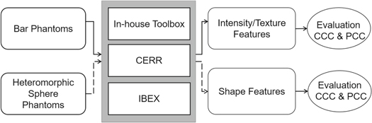
Figure 1. Overall workflow of the presented study. CCC represents for 'concordance correlation coefficient' and PCC represents for 'Pearson correlation coefficient'.
Download figure:
Standard image High-resolution image2.1. Phantom design
We designed two types of phantoms: heteromorphic sphere phantoms and bar phantoms. There were several considerations during the phantom design: (1) the feature values of the phantom should be easy to be manual verification or intuitively perceived for the convenient final validation; (2) no pre-processing (e.g. segmentation and grey level discretization) is necessary; (3) the phantom should be comprised of a series of phantoms with regular intensity, texture, and shape variations, for the convenience of characterizing the sources of variation.
2.1.1. Heteromorphic sphere phantoms
We constructed a series of heteromorphic sphere phantoms for characterizing shape features in a stochastic and iterative mechanism. The rational for this approach was to generate local topological changes on the surface of the phantoms (e.g., as shown in figure 2(a)) and study their effect on shape feature calculation. The starting point was a perfect sphere with radius of 80 voxels, which was iteratively perturbed to simulate changes in size and structure relative to baseline. In each iteration, a sphere with ten-voxel radius was stochastically attached to the surface of the previous iteration of the phantom. The voxel size of 1 mm × 1 mm × 1 mm was used in this study. In addition to the starting point, we acquired the phantoms every 500 iterations and up to 5500 iterations.

Figure 2. Illustrations of phantom design. (a) Heteromorphic sphere phantoms. (b) Bar phantoms.
Download figure:
Standard image High-resolution image2.1.2. Bar phantoms
As shown in figure 2(b), a series of bar phantoms were developed for characterizing intensity and texture features. The bar phantoms consisted of 66 × 66 × 12 voxels, with the voxel size of 1 mm × 1 mm × 2 mm. The outermost one-voxel shell was of value 0. The region of interest (ROI) was specified as the non-zero regions in the phantoms. The shell was designed to mimic the real environment in common radiomics studies. The phantoms were evenly distributed into 2, 4, 8, or 64 bars, and the grey levels of the n bars were evenly distributed between 1 and 64. The construction parameters of each phantom are shown in appendix A, Table A1.
2.2. Feature extraction
We calculated and compared 61 typical features (as shown in appendix B, Figure B1) from 3 radiomics toolboxes: (1) CERR (2) IBEX (3) MATLAB-based in-house platform (MathWorks, Natick, MA, USA). These features were with common naming conventions or different naming contentions but common feature definitions among the toolboxes. They included 22 texture features from the grey-level co-occurrence matrix (GLCOM) (Haralick and Shanmugam, 1973), 11 texture features from the grey-level run-length matrix (GLRLM) (Galloway 1975), 13 texture features from the grey-level size-zone matrix (GLSZM) (Thibault et al 2014), 5 features from the neighboring grey-level difference matrix (NGLDM) (Amadasun and King 1989), 6 shape features, and 4 intensity histogram-based features. All texture features were calculated in 3D mechanism: (1) GLCOM and GLRLM features were calculated along 13 searching directions (as shown in appendix C); and (2) GLSZM and NGLDM features were calculated with 3D-neighbor volume of 26 voxels. Note that four calculation methods were used for shape features as CERR provides two algorithms, Delaunay algorithm and marching cubes algorithm. We compared both algorithms and nominated them as CERRD and CERRM, respectively.
2.3. Evaluation on feature extraction consistency
Both concordance correlation coefficient (CCC) and Pearson correlation coefficient (PCC) were used for pair-wise comparison among the three toolboxes. CCC evaluates data reproducibility and inter-rater reliability (Lawrence 1989). High CCC indicates high degree to which the data pair lie along the line of equality (i.e. the 45° line in linear coordinate), and CCC that is not equal to 1 indicates inconsistencies between two groups of data. CCC was scored into 4 categories: (1) perfect agreement: CCC = 1; (2) strong agreement: CCC > = 0.8; (3) moderate agreement: 0.5< = CCC < 0.8; (4) weak agreement: CCC < 0.5. This scoring breakdown mechanism was adopted based on previous studies (Lafata et al 2018, 2019a, Foy et al 2018b, Parmar et al 2014). PCC measures a linear relationship which could departure from the 45° line (Lawrence 1989). The rationale of using PCC is as follows: When the results from different toolboxes do not agree exactly based on CCC, we would want to know by how much the inconsistencies would likely to affect downstream modeling results. If the features produced from two toolboxes are different values but linearly correlated, they may potentially generate similar results with respect to downstream models, relative to non-linear feature inconsistences.
3. Results
3.1. Shape features
The variations of shape features calculated from the heteromorphic sphere phantom with iteration number are shown in figure 3. The volume values calculated from the four calculation algorithms were comparable, while the surface area values increased at two different rates. Since all other shape features are correlated with volume and surface area, they also varied at two rates with iteration number.

Figure 3. Variations of shape feature values with iteration number. The feature values were normalized by the initial values (perfect sphere).
Download figure:
Standard image High-resolution imageThe CCC and PCC for each shape feature are provided in appendix D, Table D1 and D2. The CCC confirmed the trends shown in figure 3: the four methods produced similar volume (CCC > 0.98); surface area was highly reproducible (CCC > 0.99) between CERRD/in-house pair or CERRM/IBEX pair yet weakly reproducible (CCC < 0.5) between the two groups. Only 2 features, the compactness 2 between CERRM /IBEX and volume between CERRM/CERRD, demonstrated perfect agreement. Meanwhile, all four methods produced PCC > 0.8 for all shape features except compactness 1. For this feature, in-house/IBEX and CERRM /IBEX resulted in PCCs of 0.76 and 0.77, respectively. These results demonstrate that inconsistencies existed in shape feature calculations among the four methods, but the features values were usually highly linear-correlated.
3.2. Intensity and texture features
The CCC and PCC of intensity histogram-based features and texture features are provided in appendix E, Table E1. The statistical results of CCC evaluation are shown in table 1. It should be noted that IBEX calculates GLRLM features only along 0° and 90° directions and does not provide calculation of GLSZM features, therefore the CCC and PCC of GLRLM and GLSZM features related to IBEX are not applicable in this comparison.
Table 1. Percentage of score categories in CCC pair-comparison.
| Number of Features | Perfect Agreement (CCC = 1) | Strong Agreement (CCC > =0.8) | Moderate Agreement (0.5 < CCC < 0.8) | Weak Agreement (CCC < 0.5) | |
|---|---|---|---|---|---|
| CCC (IH/CERR) | 55 | 52.7% | 70.9% | 3.6% | 25.5% |
| CCC (IH /IBEX) | 31 | 45.2% | 61.3% | 0% | 38.7% |
| CCC (CERR/IBEX) | 31 | 54.8% | 61.3% | 0% | 38.7% |
Note: 'IH' represents for 'in-house' radiomics toolbox.
As seen in table 1, the percentage of perfect agreement was only 53%, 45%, and 55% for in-house/CERR, in-house/IBEX, and CERR/IBEX pairs, respectively. The average CCC reached 0.981, 0.991, and 0.998 for features with strong agreements for in-house /CERR, in-house/IBEX, and CERR/IBEX pairs. Most features demonstrated either strong agreement or weak agreement between two radiomics toolboxes. Among the features with moderate or weak CCC, only a few demonstrated a PCC lower than 0.95, which are shown in table 2. A negative PCC value indicates an inverse relationship between two features from different toolboxes. These features which were with moderate or weak agreement on CCC but high PCC demonstrated strong linear relationship, even though the feature values were not highly reproducible between two toolboxes.
Table 2. Features with Pearson correlation lower than 0.95.
| Toolboxes | Feature Name | PCC |
|---|---|---|
| IH versus CERR | Variation Of Intensity | −0.735 |
| IH versus IBEX | Differential Entropy | −0.387 |
| Info Measure Correlation1 | 0.452 | |
| Variation Of Intensity | −0.735 | |
| Coarseness | −0.381 | |
| Complexity | −0.114 | |
| CERR versus IBEX | Differential Entropy | −0.386 |
| Info Measure Correlation1 | 0.479 | |
| Busyness | −0.387 | |
| Coarseness | −0.382 | |
| Complexity | −0.113 | |
| Contrast | −0.386 |
4. Discussion
In this study, digital phantoms were developed and implemented to investigate potential inconsistencies among three different radiomics feature extraction toolboxes: CERR, IBEX, and an in-house toolbox. While all three toolboxes incorporate similar stages of computation (i.e., DICOM reading, image pre-processing, contour delineation, gray-scale re-binning, etc), the fashion in which they are implemented are often quite different. Our results demonstrate that variations exist among radiomic features derived from different toolboxes.
As mentioned above, the IBSI (Zwanenburg 2017, Zwanenburg et al 2016) greatly contributed to benchmarking radiomic extraction processes across multiple institutions. Taking a different approach to the sequential phantoms developed in our study, IBSI utilized a single cubic-like digital phantom with several discrete gray levels to achieve its goal of benchmarking. Compared to a single phantom implementation, sequential phantoms have several unique advantages: (1) they are convenient for perceptive checking, which is especially meaningful for first-order features and shape features (relative to a perfect sphere). (2) They make the task of figuring out the sources of variations relatively easy, which would be helpful for the developers of radiomics toolboxes to debug their programs. (3) They provide more information during referring other radiomics studies. Researchers could know which features could be with extraction discrepancies by the CCC evaluation, and by how much the inconsistencies are non-linear by the PCC evaluation. Beyond the merits of serial phantoms, the bar phantoms and heteromorphic sphere phantoms were designed in such shapes and textures on purpose. First, the phantoms were designed to enable easy, intuitive check on the features, considering the physical meanings and mathematical definitions of radiomics features. In particular, most shape features describe the similarity of between the ROI and a perfect sphere, hence we designed a sphere-based phantom with morphological changes. Many texture features are relevant to the homogeneity or heterogeneity of the ROI, and the computation of texture features are related to the rotational variance. Therefore, bar phantoms with a regular homogeneity change and texture variations along different axes of rotation were designed. Second, the phantoms were designed in a way that the differences will be apparent and meaningful trends will be shown. For example, the complex surface of the heteromorphic phantoms results in apparent differences caused by the different algorithms used for calculating surface area and volume. Another example is that any differences in texture feature matrix computation (e.g., GLCOM and GLRLM) will also be apparent with the bar phantoms. Third, they help in understanding mathematical interpretations of features, which is especially helpful for characterizing new feature engineering techniques. For example, our results (as shown in figure 3) demonstrated that the sphericity of the heteromorphic sphere phantoms should be maximized at a perfect sphere and should decrease as the morphology changes until saturating.
We provided two evaluation metrics- CCC and PCC. The importance of CCC and PCC depends on the specific task. For the purpose of QA, CCC is the most important evaluation criteria, since it evaluates data reproducibility. Noted that in general there is no absolute threshold indicating an acceptable degree of discrepancy, even though we scored our CCC results into different categories. PCC is informative during referring others' research findings, since researchers would want to know how much inconsistencies could exist if they used different toolboxes. If the features produced from two toolboxes do not match based on CCC but linearly correlated, they may potentially generate similar results with respect to downstream models, relative to non-linear feature inconsistences.
The use of sequential phantoms, specifically separate phantoms for different types of features, can therefore potentially provide useful information regarding feature extraction inconsistencies across toolboxes. In our study, the disagreement between feature values was driven by many different factors. First, disagreements were observed as a result of differences in mathematical definitions. For example, feature S1 (compactness1) is defined via equation (1) (Aerts et al 2014) in in-house toolbox and IBEX, yet via equation (2) (Zwanenburg et al 2016) in CERR toolbox. Feature I3 (kurtosis) by in-house toolbox and by CERR is in relationship (3). This is the reason why the I3 is in weak agreement in CCC (IH/CERR) but high Pearson correlation (PCC = 1). None of the mathematical definitions were incorrect, however, we can see the necessity of standardizing the mathematical definitions for the generalization of radiomics research findings.


Second, disagreements were observed due to different pre-processing steps inherent to different toolboxes. As shown in appendix F, Table F1–F6 features I1 (energy) from IBEX demonstrated weak agreement with the other two toolboxes. This is due to the specific gray-level re-binning method implemented in IBEX. Specifically, IBEX applies a re-binning algorithm of dividing the CT number 0-4096 into 25 bins for intensity features, except for entropy whose binning range and bin width are adjustable. In general, however, this type of disagreement could be avoided for clinical applications of radiomics research findings.
Lastly, disagreements were observed as a result of differences in calculation methods. For example, when calculating texture features from joint-probability matrices, the in-house toolbox applied a z-direction normalization factor when accounting for rotational invariance of anisotropic voxels, while CERR did not apply this correction. Another example is the calculation of surface area. As shown in figure 3, the surface area calculated from Delaunay algorithm is lower than that from marching cubes algorithm, and the difference increases with iterations. This difference could potentially be caused by the inherent characteristics of the algorithms, and they are sensitivity in deriving final values. For example, the Delaunay triangulation algorithm tends to incorrectly calculate the fine interfaces of the small attaching spheres, especially at high iteration. Therefore, while these algorithms resulted in similar volume measurements, other shape features that are formulated based on surface area and volume demonstrated larger differences at high iteration.
In addition to these findings, our results also demonstrated the significance of calculating texture features in a fully 3D fashion. In the radiomics toolboxes, feature values are calculated as the average of feature values along 13 unique axes of rotation. Figure 4 illustrates the value of feature 'GLRLM Run Length Percentage' along the 13 unique axes of rotation, where we can see the directional dependence of the feature. IBEX calculates GLRLM features only along 0° and 90° directions, which may cause inconsistencies due to not fully approximating a rotationally invariant system.
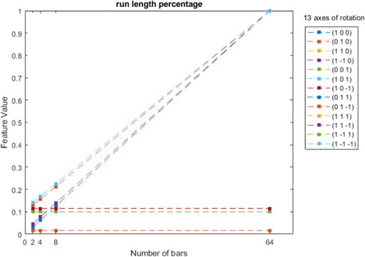
Figure 4. GLRLM Run Length Percentage feature value along 13 directions.
Download figure:
Standard image High-resolution imageWe have demonstrated that there are many sources of variation in feature extraction. Although discrepancies exist, it is important to note that the different implementations are not necessarily incorrect, as long as the software is consistent when comparing results. Researchers should be aware of the differences and consider it when building radiomic models. Additionally, how these variations would affect the clinical decision support is very much a task-based problem and worth further exploration. As concluded in previous studies (Lafata et al 2018, Foy et al 2018a), variations in feature values have been shown to affect downstream modeling results. In particular, Foy et al (Foy et al 2018a) demonstrated that features from different radiomics toolboxes affected the model performance on predicting radiation pneumonitis. Therefore, for future clinical radiomic application, the standardization or QA of radiomics toolboxes will be necessary for the reproducibility and generalization of radiomics research findings. Based on our findings, we suggest a working group for the standardized of radiomic features and the development of a protocol for the QA of radiomic applications. Digital phantoms, similar to the ones used in this study, can potentially be used as a tool for this purpose. Once researchers agree on a universal feature extraction ontology to address the mentioned disagreements, feature values extracted from the digital phantoms may serve as a warranted reference calculation.
We acknowledge that the current research only studies the variability associated with a single component of a typical radiomic pipeline. Thus, no clinical outcome comparison was involved in this study. However, variability of radiomic features with respect to image acquisition parameters, imaging modalities, preprocessing steps, or modeling algorithms could also affect final clinical decision making. Eventually the community will need to understand how different sources of variations interact to understand their aggregate behavior.
5. Conclusions
We developed a series of heteromorphic sphere phantoms and a series of bar phantoms for checking the feature extraction consistency among three radiomics toolboxes: CERR, IBEX, and an in-house toolbox. We observed inconsistent feature values and discrepancies in mathematical definition, pre-processing implementation, and calculation methods among the three toolboxes, thus demonstrating the significance of radiomics software QA. The digital phantoms can be applied as useful tools for the QA.
Appendix A
Table A1. Bar phantom construction parameters.
| Number of bars | Grey levels | Bar width (voxel) |
|---|---|---|
| 2 | 1, 64 | 32 |
| 4 | 1, 22, 43, 64 | 16 |
| 8 | 1, 10, 19, 28, 37, 46, 55, 64 | 8 |
| 64 | 1, 2, 3, ..., 64 | 1 |
Appendix B

Figure B1. Full list of features compared in this study. Colors represent feature classes.
Download figure:
Standard image High-resolution image
Appendix C
13 searching directions
Appendix D
Table D1. Pair-wise CCC on shape features.
| Feature | CCC IH/CERRD | CCC IH/CERRM | CCC IH /IBEX | CCC IBEX/CERRD | CCC IBEX/CERRM | CCC CERRD/CERRM |
|---|---|---|---|---|---|---|
| S1 | 0.978 | 0.275 | 0.352 | 0.381 | 0.092 | 0.265 |
| S2 | 0.987 | 0.570 | 0.566 | 0.564 | 1.000 | 0.567 |
| S3 | 0.975 | 0.200 | 0.193 | 0.183 | 0.998 | 0.189 |
| S4 | 0.954 | 0.046 | 0.042 | 0.035 | 0.977 | 0.039 |
| S5 | 0.992 | 0.194 | 0.183 | 0.167 | 0.995 | 0.177 |
| S6 | 0.997 | 0.997 | 0.986 | 0.996 | 0.996 | 1.000 |
Table D2. Pair-wise PCC on shape features.
| Feature | PCC IH/CERRD | PCCIH/CERRM | PCC IH /IBEX | PCC IBEX/CERRD | PCC IBEX/CERRM | PCC CERRD/CERRM |
|---|---|---|---|---|---|---|
| S1 | 0.979 | 0.995 | 0.763 | 0.827 | 0.772 | 0.991 |
| S2 | 0.987 | 0.991 | 0.991 | 0.999 | 1.000 | 0.999 |
| S3 | 0.975 | 0.994 | 0.993 | 0.978 | 1.000 | 0.980 |
| S4 | 0.957 | 0.916 | 0.900 | 0.819 | 0.999 | 0.840 |
| S5 | 0.998 | 0.997 | 0.996 | 0.994 | 1.000 | 0.995 |
| S6 | 1.000 | 1.000 | 1.000 | 1.000 | 1.000 | 1.000 |
Appendix E
Table E1. Pair-wise comparison on intensity and texture features.
| Feature | CCC IH/CERR | CCC IH /IBEX | CCC CERR/IBEX | PCC IH/CERR | PCC IH /IBEX | PCC CERR/IBEX |
|---|---|---|---|---|---|---|
| I1 | 1.000 | 0.000 | 0.000 | 1.000 | 1.000 | 1.000 |
| I2 | 1.000 | 1.000 | 1.000 | 1.000 | 1.000 | 1.000 |
| I3 | 0.023 | 1.000 | 0.023 | 1.000 | 1.000 | 1.000 |
| I4 | 1.000 | 1.000 | 1.000 | 1.000 | 1.000 | 1.000 |
| CO1 | 1.000 | 1.000 | 1.000 | 1.000 | 1.000 | 1.000 |
| CO2 | 1.000 | 1.000 | 1.000 | 1.000 | 1.000 | 1.000 |
| CO3 | 0.000 | 0.000 | 1.000 | 1.000 | 1.000 | 1.000 |
| CO4 | 1.000 | 1.000 | 1.000 | 1.000 | 1.000 | 1.000 |
| CO5 | 1.000 | 1.000 | 1.000 | 1.000 | 1.000 | 1.000 |
| CO6 | 0.996 | 0.996 | 1.000 | 0.998 | 0.998 | 1.000 |
| CO7 | 1.000 | −0.188 | −0.183 | 1.000 | −0.387 | −0.386 |
| CO8 | 0.000 | 0.000 | 0.000 | 1.000 | 1.000 | 1.000 |
| CO9 | 1.000 | 1.000 | 1.000 | 1.000 | 1.000 | 1.000 |
| CO10 | 1.000 | 0.984 | 0.983 | 1.000 | 0.999 | 0.999 |
| CO11 | 1.000 | 1.000 | 1.000 | 1.000 | 1.000 | 1.000 |
| CO12 | 1.000 | 1.000 | 1.000 | 1.000 | 1.000 | 1.000 |
| CO13 | 0.995 | 0.197 | 0.201 | 0.999 | 0.452 | 0.479 |
| CO14 | 1.000 | 1.000 | 1.000 | 1.000 | 1.000 | 1.000 |
| CO15 | 0.942 | 0.942 | 1.000 | 0.977 | 0.977 | 1.000 |
| CO16 | 0.942 | 0.942 | 1.000 | 0.977 | 0.977 | 1.000 |
| CO17 | 1.000 | 1.000 | 1.000 | 1.000 | 1.000 | 1.000 |
| CO18 | 1.000 | 1.000 | 1.000 | 1.000 | 1.000 | 1.000 |
| CO19 | 1.000 | 1.000 | 1.000 | 1.000 | 1.000 | 1.000 |
| CO20 | 1.000 | 0.975 | 0.975 | 1.000 | 0.997 | 0.997 |
| CO21 | 1.000 | 0.143 | 0.143 | 1.000 | 0.992 | 0.992 |
| CO22 | 0.116 | 0.323 | 0.128 | 1.000 | 1.000 | 1.000 |
| RL1 | 0.000 | N.A. | N.A. | 1.000 | N.A. | N.A. |
| RL2 | 0.307 | N.A. | N.A. | 0.999 | N.A. | N.A. |
| RL3 | 0.044 | N.A. | N.A. | 1.000 | N.A. | N.A. |
| RL4 | 0.359 | N.A. | N.A. | 0.999 | N.A. | N.A. |
| RL5 | 0.942 | N.A. | N.A. | 1.000 | N.A. | N.A. |
| RL6 | 1.000 | N.A. | N.A. | 1.000 | N.A. | N.A. |
| RL7 | 1.000 | N.A. | N.A. | 1.000 | N.A. | N.A. |
| RL8 | 0.848 | N.A. | N.A. | 0.970 | N.A. | N.A. |
| RL9 | 0.998 | N.A. | N.A. | 1.000 | N.A. | N.A. |
| RL10 | 0.866 | N.A. | N.A. | 1.000 | N.A. | N.A. |
| RL11 | 0.602 | N.A. | N.A. | 1.000 | N.A. | N.A. |
| SZ1 | 1.000 | N.A. | N.A. | 1.000 | N.A. | N.A. |
| SZ2 | 1.000 | N.A. | N.A. | 1.000 | N.A. | N.A. |
| SZ3 | 0.000 | N.A. | N.A. | 1.000 | N.A. | N.A. |
| SZ4 | 0.000 | N.A. | N.A. | 1.000 | N.A. | N.A. |
| SZ5 | 0.750 | N.A. | N.A. | 1.000 | N.A. | N.A. |
| SZ6 | 1.000 | N.A. | N.A. | 1.000 | N.A. | N.A. |
| SZ7 | 1.000 | N.A. | N.A. | 1.000 | N.A. | N.A. |
| SZ8 | 1.000 | N.A. | N.A. | 1.000 | N.A. | N.A. |
| SZ9 | 1.000 | N.A. | N.A. | 1.000 | N.A. | N.A. |
| SZ10 | 1.000 | N.A. | N.A. | 1.000 | N.A. | N.A. |
| SZ11 | 1.000 | N.A. | N.A. | 1.000 | N.A. | N.A. |
| SZ12 | 0.000 | N.A. | N.A. | −0.735 | N.A. | N.A. |
| SZ13 | 1.000 | N.A. | N.A. | 1.000 | N.A. | N.A. |
| ND1 | 0.000 | 0.000 | 0.000 | 1.000 | 1.000 | −0.387 |
| ND2 | 0.820 | 0.000 | 0.000 | 1.000 | −0.381 | −0.382 |
| ND3 | 0.915 | −0.108 | −0.105 | 1.000 | −0.114 | −0.113 |
| ND4 | 0.000 | 0.000 | −0.084 | 1.000 | 1.000 | −0.386 |
| ND5 | 0.058 | 0.000 | 0.000 | 1.000 | 1.000 | 1.000 |
Note: 'IH' represents for 'in-house' radiomics toolbox. IBEX calculates GLRLM features only along 0° and 90° directions and does not provide calculation of GLSZM features, therefore the CCC of GLRLM and GLSZM features related to IBEX is not applicable in this comparison.
Appendix F
Table F1. Shape feature values.
| In-house | 0.037 | 0.024 | 0.021 | 0.020 | 0.020 | 0.021 | 0.021 | 0.020 | 0.020 | 0.020 | 0.020 | 0.020 | |
|---|---|---|---|---|---|---|---|---|---|---|---|---|---|
| CERRD | 0.030 | 0.018 | 0.017 | 0.017 | 0.017 | 0.017 | 0.017 | 0.017 | 0.017 | 0.017 | 0.017 | 0.016 | |
| Compactness1 | CERRM | 0.027 | 0.007 | 0.005 | 0.004 | 0.004 | 0.004 | 0.003 | 0.003 | 0.003 | 0.003 | 0.003 | 0.003 |
| IBEX | 13.940 | 9.514 | 9.334 | 9.415 | 9.564 | 9.864 | 10.094 | 10.368 | 10.613 | 10.798 | 10.985 | 11.199 | |
| In-house | 1.512 | 0.648 | 0.511 | 0.445 | 0.469 | 0.480 | 0.477 | 0.447 | 0.439 | 0.432 | 0.439 | 0.442 | |
| Compactness2 | CERRD | 1.010 | 0.344 | 0.333 | 0.326 | 0.322 | 0.309 | 0.309 | 0.314 | 0.320 | 0.318 | 0.317 | 0.290 |
| CERRM | 0.800 | 0.059 | 0.031 | 0.021 | 0.016 | 0.014 | 0.013 | 0.011 | 0.010 | 0.009 | 0.009 | 0.008 | |
| IBEX | 0.952 | 0.069 | 0.035 | 0.023 | 0.017 | 0.015 | 0.013 | 0.011 | 0.010 | 0.009 | 0.008 | 0.008 | |
| In-house | 1.148 | 0.866 | 0.799 | 0.764 | 0.777 | 0.783 | 0.782 | 0.765 | 0.760 | 0.756 | 0.760 | 0.762 | |
| Sphericity | CERRD | 1.003 | 0.701 | 0.693 | 0.688 | 0.686 | 0.676 | 0.676 | 0.680 | 0.684 | 0.683 | 0.682 | 0.662 |
| CERRM | 0.928 | 0.389 | 0.315 | 0.278 | 0.254 | 0.243 | 0.232 | 0.226 | 0.217 | 0.211 | 0.205 | 0.200 | |
| IBEX | 0.984 | 0.411 | 0.328 | 0.285 | 0.258 | 0.244 | 0.232 | 0.225 | 0.216 | 0.209 | 0.201 | 0.196 | |
| In-house | 0.871 | 1.155 | 1.251 | 1.310 | 1.287 | 1.277 | 1.279 | 1.308 | 1.315 | 1.323 | 1.316 | 1.313 | |
| Sphere Dispropor--tion | CERRD | 0.997 | 1.427 | 1.443 | 1.454 | 1.458 | 1.478 | 1.479 | 1.472 | 1.463 | 1.465 | 1.467 | 1.510 |
| CERRM | 1.077 | 2.568 | 3.170 | 3.600 | 3.933 | 4.115 | 4.304 | 4.431 | 4.606 | 4.750 | 4.883 | 5.009 | |
| IBEX | 1.017 | 2.434 | 3.051 | 3.513 | 3.880 | 4.091 | 4.307 | 4.451 | 4.621 | 4.791 | 4.963 | 5.098 | |
| In-house | 1197 | 1526 | 1824 | 1995 | 2155 | 2322 | 2521 | 2688 | 2853 | 2992 | 3124 | 1197 | |
| CERRD | 1484 | 1764 | 2014 | 2237 | 2459 | 2640 | 2787 | 2934 | 3091 | 3257 | 3507 | 1484 | |
| Surface Area | CERRM | 2670 | 3874 | 4989 | 6031 | 6844 | 7680 | 8392 | 9240 | 10024 | 10843 | 11632 | 2670 |
| IBEX | 2511 | 3686 | 4800 | 5848 | 6674 | 7528 | 8248 | 9077 | 9888 | 10757 | 11551 | 2511 | |
| In-house | 3134 | 4007 | 4888 | 5736 | 6514 | 7268 | 7959 | 8688 | 9414 | 10192 | 10915 | 3134 | |
| CERRD | 3152 | 4017 | 4851 | 5647 | 6378 | 7088 | 7750 | 8449 | 9118 | 9839 | 10522 | 3152 | |
| Volume | CERRM | 3152 | 4017 | 4851 | 5647 | 6378 | 7088 | 7750 | 8449 | 9118 | 9839 | 10522 | 3152 |
| IBEX | 3115 | 3947 | 4749 | 5502 | 6198 | 6872 | 7501 | 8186 | 8817 | 9488 | 10143 | 3115 |
Note: CERRD represents for using Delaunay algorithm in CERR for calculating shape features, and CERRM represent for using marching cubes algorithm.
Table F2. First order feature values.
| In-House | CERR | IBEX | ||||||||||
|---|---|---|---|---|---|---|---|---|---|---|---|---|
| Feature | 2 | 4 | 8 | 64 | 2 | 4 | 8 | 64 | 2 | 4 | 8 | 64 |
| Energy | 8.39E + 07 | 6.58E + 07 | 6.07E + 07 | 5.72E + 07 | 8.39E + 07 | 6.58E + 07 | 6.07E + 07 | 5.72E + 07 | 1.07E + 06 | 1.07E + 06 | 1.07E + 06 | 1.07E + 06 |
| Entropy | 1.00 | 2.00 | 3.00 | 6.00 | 1.000 | 2.000 | 3.000 | 5.969 | 1.000 | 2.000 | 3.000 | 6.000 |
| Kurtosis | 1.00 | 1.64 | 1.76 | 1.80 | −2.000 | −1.360 | −1.238 | −1.201 | 1.000 | 1.640 | 1.762 | 1.799 |
| Skewness | 0.00 | 0.00 | 0.00 | 0.00 | 0.000 | 0.000 | 0.000 | 0.000 | 0.000 | 0.000 | 0.000 | 0.000 |
Table F3. GLCOM feature values.
| In-House | CERR | IBEX | ||||||||||
|---|---|---|---|---|---|---|---|---|---|---|---|---|
| Feature | 2 | 4 | 8 | 64 | 2 | 4 | 8 | 64 | 2 | 4 | 8 | 64 |
| Auto Correlation | 2026.265 | 1595.147 | 1471.971 | 1389.853 | 2026.692 | 1595.385 | 1472.154 | 1390.000 | 2026.728 | 1595.405 | 1472.169 | 1390.012 |
| Cluster Prominence | 1.56E + 07 | 7.78E + 06 | 4.93E + 06 | 3.21E + 06 | 1.56E + 07 | 7.78E + 06 | 4.93E + 06 | 3.21E + 06 | 1.56E + 07 | 7.78E + 06 | 4.93E + 06 | 3.21E + 06 |
| Cluster Shade | 0.000 | 0.000 | −0.001 | 0.000 | 0.000 | 0.000 | 0.000 | 0.000 | 0.000 | 0.000 | 0.000 | 0.000 |
| Cluster Tendency | 3924.529 | 2170.412 | 1669.235 | 1335.118 | 3925.385 | 2171.077 | 1669.846 | 1335.692 | 3925.457 | 2171.133 | 1669.898 | 1335.741 |
| Contrast | 44.471 | 14.824 | 6.353 | 0.706 | 43.615 | 14.538 | 6.231 | 0.692 | 43.543 | 14.514 | 6.220 | 0.691 |
| Correlation | 0.978 | 0.986 | 0.992 | 0.999 | 0.978 | 0.987 | 0.993 | 0.999 | 0.978 | 0.987 | 0.993 | 0.999 |
| Difference Entropy | 0.083 | 0.195 | 0.355 | 0.000 | 0.081 | 0.191 | 0.348 | 0.000 | 0.087 | 0.209 | 0.391 | 0.892 |
| Dissimilarity | 0.706 | 0.706 | 0.706 | 0.706 | 0.692 | 0.692 | 0.692 | 0.692 | 0.691 | 0.691 | 0.691 | 0.691 |
| Energy | 0.489 | 0.234 | 0.107 | 0.010 | 0.489 | 0.234 | 0.107 | 0.010 | 0.489 | 0.234 | 0.107 | 0.006 |
| Entropy | 1.083 | 2.215 | 3.419 | 6.690 | 1.081 | 2.210 | 3.411 | 6.677 | 1.086 | 2.225 | 3.446 | 7.510 |
| Homogeneity1 | 0.989 | 0.968 | 0.929 | 0.647 | 0.989 | 0.969 | 0.931 | 0.654 | 0.989 | 0.969 | 0.931 | 0.654 |
| Homogeneity2 | 0.989 | 0.966 | 0.923 | 0.647 | 0.989 | 0.967 | 0.924 | 0.654 | 0.989 | 0.967 | 0.924 | 0.654 |
| InfoMeasure Correlation1 | −0.917 | −0.893 | −0.860 | −0.885 | −0.919 | −0.895 | −0.863 | −0.886 | −0.914 | −0.887 | −0.851 | −0.748 |
| InfoMeasure Correlation2 | 0.916 | 0.985 | 0.997 | 1.000 | 0.916 | 0.985 | 0.997 | 1.000 | 0.916 | 0.986 | 0.997 | 1.000 |
| Inverse Difference Moment Normalized | 0.994 | 0.997 | 0.998 | 1.000 | 0.995 | 0.997 | 0.999 | 1.000 | 0.995 | 0.997 | 0.999 | 1.000 |
| Inverse Difference Normalized | 0.994 | 0.992 | 0.990 | 0.989 | 0.995 | 0.992 | 0.991 | 0.989 | 0.995 | 0.992 | 0.991 | 0.989 |
| Inverse Variance | 0.000 | 0.000 | 0.001 | 0.706 | 0.000 | 0.000 | 0.001 | 0.692 | 0.000 | 0.000 | 0.001 | 0.691 |
| Maximum Probability | 0.494 | 0.242 | 0.115 | 0.010 | 0.495 | 0.242 | 0.115 | 0.010 | 0.495 | 0.242 | 0.115 | 0.007 |
| Sum Average | 65.000 | 65.000 | 65.000 | 65.000 | 65.000 | 65.000 | 65.000 | 65.000 | 65.000 | 65.000 | 65.000 | 65.000 |
| Sum Entropy | 1.072 | 2.181 | 3.340 | 5.984 | 1.070 | 2.178 | 3.334 | 5.984 | 1.076 | 2.195 | 3.376 | 6.876 |
| Sum Variance | 3924.529 | 2170.412 | 1669.235 | 1335.118 | 3925.385 | 2171.077 | 1669.846 | 1335.692 | 8011.710 | 6115.584 | 5467.415 | 4714.126 |
| Variance | 1983.530 | 1537.590 | 1410.180 | 1325.240 | 992.250 | 546.404 | 419.019 | 334.096 | 3925.457 | 2171.133 | 1669.898 | 1335.741 |
Table F4. GLRLM feature values.
| In-House | CERR | |||||||
|---|---|---|---|---|---|---|---|---|
| Feature | 2 | 4 | 8 | 64 | 2 | 4 | 8 | 64 |
| SRE | 0.050 | 0.068 | 0.091 | 0.712 | 0.046 | 0.046 | 0.046 | 0.046 |
| LRE | 775.710 | 588.919 | 527.330 | 498.253 | 532.084 | 406.098 | 361.074 | 336.254 |
| GLNU | 0.033 | 0.021 | 0.014 | 0.009 | 0.500 | 0.250 | 0.125 | 0.016 |
| RLNU | 0.026 | 0.029 | 0.048 | 0.565 | 0.461 | 0.437 | 0.478 | 0.935 |
| RP | 0.085 | 0.106 | 0.148 | 0.727 | 0.099 | 0.119 | 0.159 | 0.719 |
| LGLRE | 0.500 | 0.251 | 0.127 | 0.025 | 0.500 | 0.251 | 0.127 | 0.025 |
| HGLRE | 2048.500 | 1607.500 | 1481.500 | 1397.500 | 2048.500 | 1607.500 | 1481.500 | 1397.500 |
| SRLGLE | 0.025 | 0.017 | 0.012 | 0.018 | 0.030 | 0.020 | 0.014 | 0.018 |
| SRHGLE | 102.949 | 108.569 | 134.187 | 995.507 | 123.624 | 130.967 | 161.102 | 979.291 |
| LRLGLE | 387.950 | 147.650 | 66.959 | 12.685 | 266.107 | 101.814 | 45.848 | 8.561 |
| LRHGLE | 1.59E + 06 | 9.47E + 05 | 7.81E + 05 | 6.96E + 05 | 1.09E + 06 | 6.53E + 05 | 5.35E + 05 | 4.70E + 05 |
Note: IBEX calculated GLRLM only along 0 and 90 degrees.
Table F5. GLSZM feature values.
| In-House | CERR | |||||||
|---|---|---|---|---|---|---|---|---|
| Feature | 2 | 4 | 8 | 64 | 2 | 4 | 8 | 64 |
| SZE | 0.000 | 0.000 | 0.000 | 0.000 | 0.000 | 0.000 | 0.000 | 0.000 |
| LZE | 4.19E + 08 | 1.05E + 08 | 2.62E + 07 | 4.10E + 05 | 4.19E + 08 | 1.05E + 08 | 2.62E + 07 | 4.10E + 05 |
| GLNU | 0.000 | 0.000 | 0.000 | 0.000 | 0.500 | 0.250 | 0.125 | 0.016 |
| SZNU | 0.000 | 0.000 | 0.000 | 0.001 | 1.000 | 1.000 | 1.000 | 1.000 |
| SP | 0.000 | 0.000 | 0.000 | 0.001 | 0.000 | 0.000 | 0.000 | 0.002 |
| LGLSE | 0.500 | 0.251 | 0.127 | 0.025 | 0.500 | 0.251 | 0.127 | 0.025 |
| HGLSE | 2048.500 | 1607.500 | 1481.500 | 1397.500 | 2048.500 | 1607.500 | 1481.500 | 1397.500 |
| SSLGLE | 0.000 | 0.000 | 0.000 | 0.000 | 0.000 | 0.000 | 0.000 | 0.000 |
| SSHGLE | 0.000 | 0.000 | 0.000 | 0.003 | 0.000 | 0.000 | 0.000 | 0.003 |
| LSLGLE | 2.10E + 08 | 2.63E + 07 | 3.33E + 06 | 1.04E + 04 | 2.10E + 08 | 2.63E + 07 | 3.33E + 06 | 1.04E + 04 |
| LSHGLE | 8.59E + 11 | 1.69E + 11 | 3.88E + 10 | 5.72E + 08 | 8.59E + 11 | 1.69E + 11 | 3.88E + 10 | 5.72E + 08 |
| VoI | 0.001 | 0.002 | 0.003 | 0.008 | 992.250 | 551.250 | 425.250 | 341.250 |
| VoA | 0.000 | 0.000 | 0.000 | 0.000 | 0.000 | 0.000 | 0.000 | 0.000 |
Note: IBEX does not include the computation of GLSZM features.
Table F6. NGTDM feature values.
| In-House | CERR | IBEX | ||||||||||
|---|---|---|---|---|---|---|---|---|---|---|---|---|
| Feature | 2 | 4 | 8 | 64 | 2 | 4 | 8 | 64 | 2 | 4 | 8 | 64 |
| Busyness | 307.333 | 91.831 | 25.479 | 0.195 | 222.561 | 66.768 | 18.547 | 0.008 | 291.892 | 29.717 | 5.120 | 0.000 |
| Coarseness | 0.000 | 0.000 | 0.000 | 0.004 | 0.000 | 0.000 | 0.000 | 0.094 | 0.000 | 0.000 | 0.000 | 1.00E + 10 |
| Complexity | 0.000 | 0.000 | 0.000 | 0.003 | 43.132 | 67.094 | 123.234 | 33.593 | 80.453 | 127.495 | 236.227 | 0.000 |
| Contrast | 1172.604 | 108.140 | 17.856 | 0.088 | 679.330 | 62.901 | 10.398 | 0.003 | 633.565 | 83.898 | 15.654 | 0.000 |
| Texture Strength | 0.205 | 0.229 | 0.353 | 5.128 | 0.283 | 0.315 | 0.485 | 127.988 | 0.216 | 0.235 | 0.358 | 7.33E + 14 |